GNSS/INS Integration Based on Machine Learning LightGBM Model for Vehicle Navigation

Abstract

To solve the problem of data accuracy degradation of vehicle GNSS/INS integrated navigation systems when the GNSS signal is unavailable or there is a GNSS outage, this paper improves the existing GNSS/INS integration methodology for land vehicle navigation based on the AI method. First, a GNSS/INS integration methodology for land vehicle navigation based on position update architecture (PUA) using LightGBM regression for predicting the position of a vehicle during a GNSS outage is presented. It uses LightGBM to model the relationship between INS data and vehicle position changes. On-board INS and GNSS data are collected when the GNSS signal is available and are used to train the PUA-LightGBM model; in the event of a GNSS outage, INS data are used as the input to the PUA-LightGBM to predict the change in vehicle position. Second, a vehicle navigation data acquisition system was designed for model validation. This included a self-developed GNSS/INS integrated navigation system and a Novatel pwrpak7-e1 GNSS/INS integrated navigation system for data acquisition on six road segments. Finally, the collected data were used for machine learning training of the PUA-LightGBM model and the existing PUA-RandomForest model. As a result, the PUA-LightGBM predicts the vehicle position with less error in the event of a GNSS outage and takes less time to train. It was also demonstrated that by allowing the model to be dynamically trained or updated while the vehicle is moving the PUA-LightGBM could adapt perfectly to the predictions of vehicle position changes in different complex road segments.

1. Introduction

Navigation and positioning are among the most widely used technologies in intelligent transportation systems, advanced vehicle control, and vehicle safety systems [1]. The main idea behind their algorithms is to use satellite data and vehicle dynamics data to calculate the current specific position of the vehicle. An algorithm’s robustness determines the accuracy of the information output from the vehicle navigation system and its ability to adapt to the environment. GNSS/INS integrated navigation is a low-cost, highly accurate, and versatile integrated navigation solution [2]. Global navigation satellite systems (GNSS) provide real-time information on the position of a vehicle, primarily via satellites. The inertial navigation system first gathers information about angular and linear motion relative to inertial space. It then uses inertial navigation differential equations to calculate vehicle speed and position changes. The GNSS and INS are complementary in many ways [3]: (1) The raw vehicle dynamics data measured by the INS are often noisy. The vehicle position information obtained through independent INS solving can drift over time, requiring external assistance to calibrate the INS data. GNSS systems, on the other hand, can provide long-term stable data when the signal is available and can be used to limit INS errors. (2) There could be GNSS outages in practical operation due to signal blockage or interference, such as the presence of buildings, tunnels, forest cover, etc. In this case, the vehicle cannot obtain the data provided by the GNSS. Hence, continuity data provided by the INS can compensate for the lack of position data in the event of a GNSS outage. (3) The data provided by the GNSS for the vehicle are updated less frequently, while the INS provides accurate short-term data at a very high rate, which can be used to interpolate GNSS trajectories. (4) The INS provides the complete vehicle state (e.g., position, speed, attitude, etc.), whereas a single GNSS receiver cannot provide angular information about the vehicle. These are also the reasons for creating vehicle integrated navigation algorithms that integrate GNSS and INS. However, the accuracy of the integrated navigation algorithm could be inevitably reduced by a long-time outage of GNSS. As a result, the solution to this problem has emerged as a hot topic in integrated navigation algorithm research.

The approaches to vehicle integrated navigation algorithms can be classified into two categories. One category is the vehicle integrated navigation algorithms based on Bayesian filtering techniques. Kalman filtering (KF) is one of the most common implementations. Liu et al. applied a dual-filter smoother to an extended Kalman filter (EKF)-based INS/GPS integrated navigation algorithm for vehicles. The authors found that the algorithm provided accurate navigation parameters in the presence of GPS signal blockage, thereby improving the overall data fusion [4]. Yang et al. proposed a MEMS-INS/GNSS integrated navigation algorithm for vehicles combined with Allan variance analysis under non-complete constraints. The resulting algorithm is applicable to the loose/tight integrated navigation method for vehicles with specific fault detection and troubleshooting capability [5]. Sasani et al. proposed the attitude and heading reference system (AHRS) algorithm for an INS/GPS loose integrated navigation system, which was found to suppress the divergence of the INS solution during a GPS outage [6]. Wang et al. proposed an SINS/OD integrated navigation algorithm for vehicles based on the state transformation extended Kalman filter (ST-EKF). The authors discovered that it achieved higher positioning and heading angle accuracy than the conventional EKF algorithm [7]. Cui et al. used an improved cubature Kalman filter (CKF) algorithm based on the sigma point update framework for GNSS/INS integrated navigation and found that it improved the reliability of the navigation system in a GNSS-challenged environment [8]. Bijjahalli and Sabatini proposed a novel low-cost high-performance vehicle integrated navigation algorithm. It employed EKF to fuse data from GNSS, INS, visual odometry, and vehicle dynamics models (as virtual sensors) [9]. The other category is artificial intelligence (AI) technology-based integrated navigation algorithms for vehicles, which aim to find linear and non-linear relationships between sensor data during vehicle operation, thus completing the process of data fusion. Chiang et al. used multilayer feedforward neural networks and backpropagation learning algorithms to improve the INS/DGPS integrated navigation method for vehicles. The resulting algorithm eliminates the effects of neural network parameters and random noise on positioning accuracy [10]. Aggarwal et al. proposed a D-S neural network for GPS/INS data fusion by combining D-S evidence theory with a neural network model. The authors found that the model improved the positioning accuracy of the vehicle integrated navigation system under GPS outage conditions [11]. Noureldin et al. implemented an autoregressive process in a stochastic modeling approach based on microelectromechanical systems inertial sensor (MEMS-INS) errors to reduce INS errors. The authors used AI to improve the accuracy of information fusion by enhancing the conventional KF module, resulting in improved performance of a low-cost MEMS-INS/GPS integrated navigation system for vehicles [12]. Chiang and Huang proposed an INS/GPS integrated navigation method that combines artificial neural networks and uses historical information. This method prevents the continuous growth of INS errors when GPS is unavailable for long periods [13]. Yue et al. proposed a two-layer, highly robust algorithm for vehicle integrated navigation systems that fuses GNSS and INS data via support vector machine regression (SVR) and adaptive Kalman filtering (AKF). This resulted in an algorithm that improves vehicle integrated navigation system positioning accuracy when GNSS signals are weak [14]. Liu et al. proposed a GPS/INS neural network (GI-NN) deep learning network structure as an INS aid when GPS is unavailable; this algorithm uses historical data from the IMU and exploits both spatial and temporal features in the IMU to achieve better localization results [15]. Using a T2FHNN (type-2 fuzzy Hammerstein neural network), Khankalantary et al. proposed a data fusion scheme for a SINS/GNSS integrated navigation system with better navigation accuracy and stability [16].

In summary, some researchers have made significant progress in improving vehicle positioning accuracy through improved integrated navigation algorithms. However, little information is available on vehicle integrated navigation algorithms based on efficient AI methods. The machine learning methods used in the existing literature for vehicle position prediction models almost did not consider the efficiency optimization issue, such as the cost of time and computational resources required for model training [12,15]. In addition, most previous AI models for predicting a vehicle’s position in the event of a GNSS outage cannot be updated online after the initial machine learning training. This results in these models only having good position prediction accuracy when the vehicle is driving on certain types of road segments covered in the training set. Moreover, the models cannot adapt to complex and dynamic changes in road segments. Overall, these models lack robustness. The AI method based on an improved position update architecture (PUA) for GNSS/INS integrated navigation can predict the position of a vehicle in the case of a GNSS outage. As a result, the objective of this study is to propose a new LightGBM machine learning algorithm based on an improved PUA for GNSS/INS integrated navigation that predicts vehicle position in the event of a GNSS outage. Additionally, the study proposes to solve the problem of the inefficient model training used in AI-based integrated navigation algorithms by improving model training efficiency. Furthermore, the PUA-LightGBM model is being proposed for the first time.

The structure of the paper is as follows: The LightGBM framework and the PUA-LightGBM model are described in Section 2. Section 3 describes the methodology and process of the experiments and the workflow of the PUA-LightGBM model in detail. The results and discussions of the experiments are presented in Section 4. Section 5 provides a conclusion.

2. Introduction to LightGBM Machine Learning Model Based on PUA

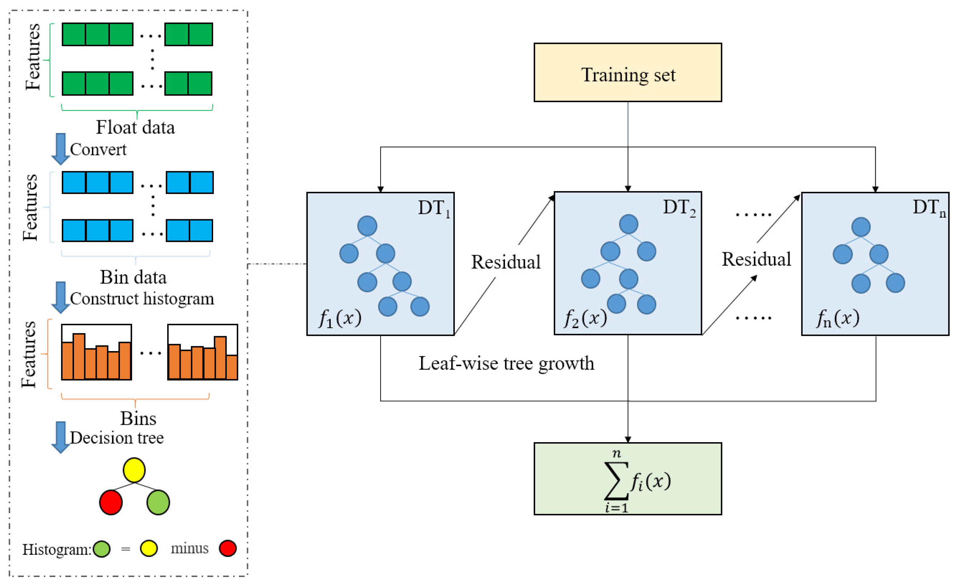
2.1. LightGBM Machine Learning Model

Gradient boosting decision tree (GBDT) is a common machine learning model used in artificial intelligence that employs several basic learners that are iteratively trained to produce the optimal model. LightGBM is a distributed and efficient framework for implementing the gradient boosted decision tree (GBDT) algorithm [17], which fits a new decision tree by approximating the negative gradient of the loss function as the residual of the current decision tree.

To improve the efficiency of machine learning model training while losing as little accuracy as possible in model prediction, the following seven optimization methods exist for LightGBM: (1) histogram-based decision tree algorithm, (2) gradient-based one-side sampling (GOSS), (3) exclusive feature bundling (EFB), (4) leaf-wise with max depth limitation, (5) categorical feature support, (6) parallel learning support, and (7) increase cache hit chance. Methods (1)–(4) are optimization algorithms, and (5)–(7) are optimizations for engineering applications.

GOSS and EFB, two main techniques used by LightGBM, improve efficiency by reducing the number of samples and features, respectively. The GOSS algorithm retains all instances with large gradients and samples with small gradients at random. EFB bundles mutually exclusive features and can losslessly reduce feature dimensionality.

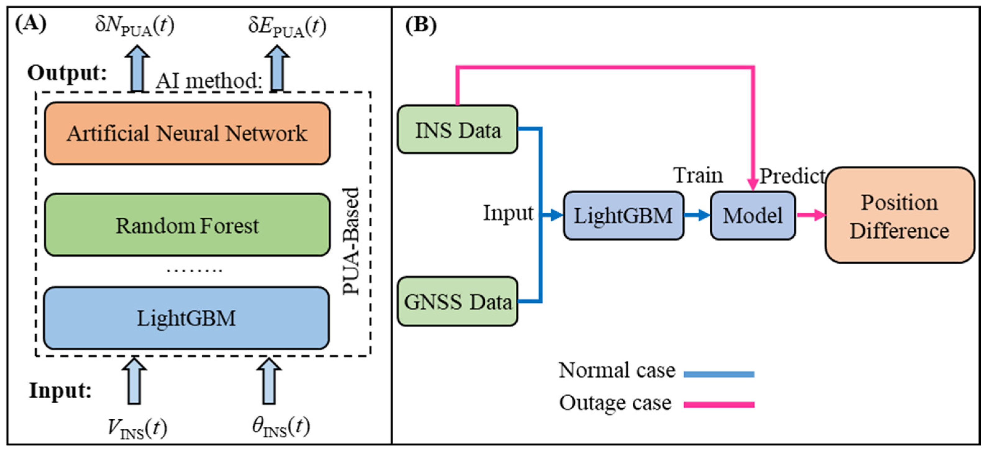
2.2. Position Update Architecture and PUA-LightGBM Model

The position update architecture is a data fusion architecture for GNSS/INS integrated navigation that uses the AI method, which defines the AI-based integrated navigation model’s inputs and outputs (Figure 1A). The architecture trains the AI model based on INS data and GNSS data, with the inputs to the model being the velocity (V_INS) and azimuth (θ_INS) given by the INS and the outputs being the differences in longitude (δE) and latitude (δN) between the two epochs. Based on the linear and non-linear relationships between the motion data and vehicle position coordinates, PUA provides a training model for predicting vehicle position changes. Hence, it is reasonable to use PUA to determine the inputs and outputs of AI. PUA makes it possible to apply AI methods to find relationships between vehicle dynamics data and position changes [18]. Initially, El-Sheimy et al. implemented an AI-based integrated navigation algorithm using ANN and PUA; in addition, AI-based integrated navigation algorithms using PUA have been proposed successively: DSNN [11], RFR [19], DS-SVM [20], etc.

This study proposes to use the PUA-based LightGBM machine learning model to predict changes in vehicle position during GNSS outage conditions. During vehicle operation, the data from the INS are combined with data from the GNSS to construct a training dataset and train a position change prediction model. When there is a GNSS outage, the INS data are used in the model to predict the change in vehicle position in real-time, as shown in Figure 1B. It is important to note that this paper uses vehicle three-axis acceleration as a feature input based on PUA. One of the main advantages of LightGBM is its high training efficiency [17]. From a practical deployment point of view, LightGBM models for vehicle position prediction in the event of a GNSS outage could collect more data. In this way, the model can update or expand the dataset while the vehicle moves, allowing it to be retrained at a lower cost and with greater adaptability.

3. Experimental Analysis and Method

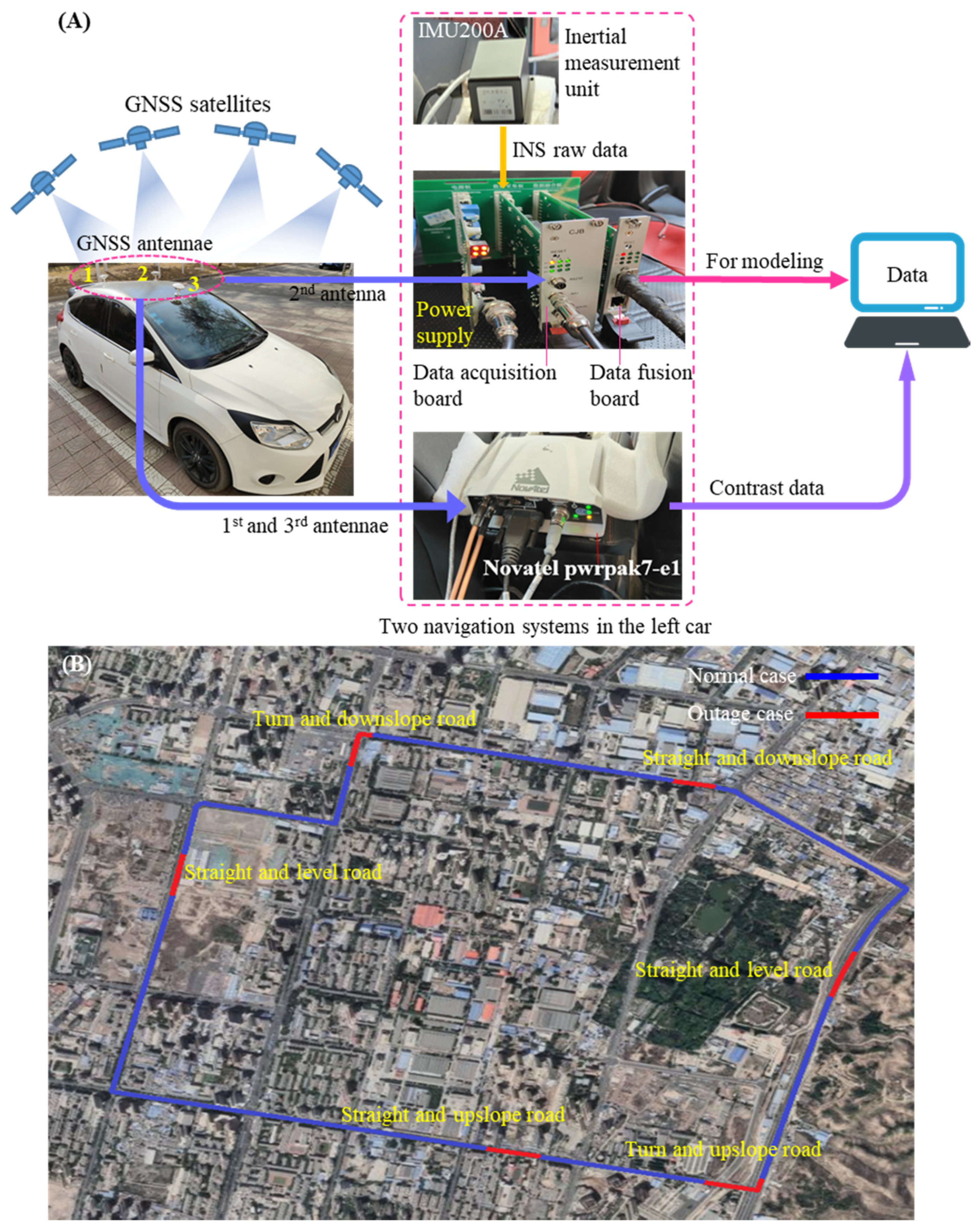
3.1. Data Acquisition

A vehicle navigation data acquisition system was designed to acquire vehicle dynamics and position data before and after the GNSS outage (Figure 2A). The system consisted of a self-developed GNSS/INS integrated navigation system (Kalman-filter-based, loosely coupled integration is used), a Novatel pwrpak7-e1 GNSS/INS integrated navigation system, and a computer. The self-developed GNSS/INS integrated navigation system included a No. 2 satellite antenna, MEMS inertial measurement unit, data acquisition board, data fusion board, and power supply unit. The data acquisition board was equipped with an integrated UB4B0M GNSS board (accuracy: better than 1.5 m for single-point positioning). The IMU200A inertial measurement unit (IMU) consisted of a gyroscope (range, ±300°/s; zero bias, 25.2°/hr; angular random walk, 144°/√hr) and an accelerometer (range, ±17 g; zero bias, 0.2 mg; velocity random walk, 12 m/s/√hr), which were fixed to a platform in the vehicle. Foam was used as a buffer material between the IMU and the platform to minimize external interference during IMU operation. Its working process was as follows: While the vehicle was moving, the No. 2 antenna installed on the vehicle’s roof searched for and tracked satellite signals. When the number of satellites searched reached four or more, the GNSS board embedded in the data acquisition board demodulated the received signals. Then, it calculated the GNSS data, which included the vehicle’s position coordinates. Simultaneously, the vehicle’s three-axis angular motion data and three-axis acceleration data output from the IMU were transmitted in real time to the data acquisition board, which intercepted and converted the GNSS data and INS raw data (IMU output) to the preset data format to complete the data acquisition process. Then, the pre-processed data were transferred to the data fusion board, where they were solved and fused to obtain the final GNSS and INS data. Subsequently, these data were transferred to the computer via the serial port of the data fusion board.

The Novatel pwrpak7-e1 GNSS/INS integrated navigation system consisted of No. 2 and No. 3 satellite antennas, a Novatel pwrpak7-e1 navigation unit with an integrated satellite receiver, and an Epson G320 MEMS-IMU (gyroscope: range, ±150°/s; zero bias, 3.5°/hr; angle random walk, 0.1°/√hr. Accelerometer: range, ±5 g; zero bias, 0.1 mg; velocity random walk, 0.5 m/s/√hr). It was possible to capture a vehicle’s trajectory, i.e., its location, with greater accuracy. The procedure was as follows: The No. 1 and No. 3 satellite antennas searched for and track the satellite signals. When the satellite positioning conditions were met, the Novatel pwrpak7-e1 performed the initial alignment to establish the initial INS benchmark, then completed the process of collecting, calculating, and fusing the GNSS and INS data and finally transmitted the data to the computer via the communication interface.

For the experiments, an open closed-loop urban road trajectory (perimeter x road width: 8168.0 × 20.6 m) was first selected (Figure 2B) to ensure that GNSS outages would not occur automatically. While the vehicle was moving and the GNSS signal was available, the position, speed, heading angle, pitch angle, and three-axis acceleration data were collected simultaneously at a frequency of 50 Hz by two integrated navigation systems installed on the vehicle. The data collected by the self-developed integrated navigation system were then used to build a training set for the LightGBM model, which was used to predict vehicle position in the event of a GNSS outage. Furthermore, to closely match all realistic driving scenarios encountered by a typical land vehicle, the data acquisition board of the self-developed integrated navigation system was manually disconnected from the satellite antenna in several scenarios. These scenarios included uphill straight, uphill bend, downhill straight, downhill bend, and two flat straight segments, which simulated six GNSS outage situations encountered by the vehicle, with each outage lasting 20 s. When simulating an outage in the self-developed integrated navigation system, only the INS system can properly output data, as the input of the LightGBM model for vehicle position prediction is under GNSS outage.

Because the outage would not occur in regular operation when a Novatel pwrpak7-e1 integrated navigation system was employed, it provided accurate vehicle position data throughout, which were used as a baseline reference against the predicted output of the LightGBM machine learning model.

3.2. Model Training

First, data pre-processing was performed. A dataset was constructed using the output data of the self-developed integrated navigation system; when the GNSS signal was available, incomplete strips of data were removed. Then, 80% of the dataset was divided into a training set, and the remaining 20% was used as a test set. The latitude and longitude data were compared to obtain the differences in longitude and latitude between the two epochs. It is worth noting that LightGBM is a high-performance framework for implementing GBDT, which is a tree model. Because the numerical scaling of the tree model does not affect the position of the split point or its structure, data normalization is not required. The training environment used was Windows 10 with an Intel i7-6700HQ processor, and the programming language was Python version 3.7 (Python Software Foundation, Fredericksburg, VA, USA).

The LightGBM model training process was then carried out, as shown in Figure 3 [21]. The inputs and outputs of the PUA-LightGBM model for vehicle position prediction in the event of a GNSS outage were determined according to Section 2.2. This means that the inputs were the velocity (V_INS) and azimuth (θ_INS) given by the INS and the three-axis acceleration of the vehicle, and the outputs were the differences in longitude (δE) and latitude (δN) between the two epochs. The longitude difference prediction and latitude difference prediction models were trained separately to implement a multiple-output regression. The parameter settings used in the model training and the descriptions of the relevant parameters are given in

Table 1. The parameters of the LightGBM model.

Parameter Name	Value	Parameter Implication
learning_rate	0.05	Learning rate
num_leaves	63	The number of leaves in a tree
num_iterations	300	Number of basic learners
bagging_fraction	0.8	The fraction of data to be considered for each iteration.
feature_fraction	0.9	The fraction of features to be considered in each iteration.

.

The output data were first used to initialize a regression decision tree (DT) based on the loss function. Following that, n regression decision trees were created. A negative gradient, or pseudo-residual, was calculated using the output value of the initialized DT with the set sample output value. This residual was then used as the output value of the set sample to train the first DT. The best split point needed to be found when training the DT, and LightGBM discretized the continuous floating-point feature values and generated a histogram (bins). As the data were traversed, the cumulative statistics of each discrete value in the histogram were counted. Feature selection was accomplished by traversing the histogram based on the discrete values to determine the best split point. The algorithm cost O(#data × #feature) for histogram building and O(#bin × #feature) for split point finding. Since #bin is usually much smaller than #data, the histogram building dominated the computational complexity [17]. DT growth employs a leaf-wise technique, which locates and divides the leaf node with the maximum splitting gain relative to the present leaf node. In addition, during DT construction, the histogram of a leaf node can be obtained from the difference between its parent node’s histogram and its sibling node’s histogram. When DT reaches a depth limit or a limit on the number of leaf nodes, the residuals are fitted by assigning leaf node weights to fit this time. After training, the LightGBM model for vehicle position prediction in the event of a GNSS outage can be updated, and the process can be repeated until n regression decision trees are constructed. Following this process, the final LightGBM model for vehicle location prediction in the event of a GNSS outage was generated. In Figure 3, $f_i(x$) is the output of DT_i. The final output of the LightGBM model for vehicle position prediction in the event of a GNSS outage is ${\sum }_{i=1}^n{f}_i(x)$, which is the prediction of the differences in longitude (δE) or latitude (δN).

3.3. Model Predictions

The model is ready for use once it has been trained. When there is a GNSS outage, the IMU can continue to work regardless of the external environment. The velocity (V_INS) and azimuth (θ_INS) provided by INS as well as the vehicle’s three-axis acceleration were employed in the model to obtain the model’s prediction of the differences in longitude (δE) and latitude (δN) between the two epochs. The longitude and latitude information provided before the GNSS outage were added to the prediction model’s longitude difference and latitude difference outputs, respectively, to obtain the vehicle’s latitude and longitude location information.

In this study, the performance of the GNSS outage position prediction model was evaluated by two metrics: the root mean square error (RMSE) and the coefficient of determination (R²), which are both commonly used in regression tasks. The equations are shown in Equations (1) and (2).

$$RMSE=\sqrt{\frac{1}{n}{\displaystyle \sum }_{i=1}^n{\left(y_i-{\widehat{y}}_i\right)}^2}$$

(1)

$$R^2=1-\frac{{\sum }_{i=1}^n{\left(y_i-{\widehat{y}}_i\right)}^2}{{\sum }_{i=1}^n{\left(y_i-{\overline{y}}_i\right)}^2}$$

(2)

where n is the total number of data points, $y_i$ is the actual value, ${\widehat{y}}_i$ is the predicted value, ${\overline{y}}_i$ is the mean of the observed data, RMSE is the root mean square error, and $R^2$ is the coefficient of determination. The smaller the RMSE value, the higher the model prediction accuracy; the closer the $R^2$ value is to 1, the better the model fits the data.

In practical application, the model is used to predict the position and trajectory of a vehicle when there is a GNSS outage, and it is compared with the actual vehicle trajectory. Then, it gives the average error of the predicted trajectory compared to the real trajectory. Model training time is critical in practice because the data acquisition system can capture new data that are generated while the vehicle moves with a strong GNSS signal. A subset of this new data can be used to augment the dataset. The shorter the training time for each model, the less time it takes to retrain the LightGBM model for vehicle position prediction during a GNSS outage. This means new models can be deployed faster and adapt to more driving conditions. As a result, the training time of the model was also used as the final evaluation metric.

4. Results and Discussion

4.1. Performance of the PUA-LightGBM Model

Table 2. Performance comparison of the PUA-LightGBM model to the PUA-RandomForest model.

Model Name	RMSE	R2	Training Time (s)
PUA-LightGBM (δE)	1.927 × 10−7	0.983	1.563
PUA-LightGBM (δN)	1.334 × 10−7	0.986	1.513
PUA-RandomForest	1.417 × 10−7	0.989	83.082

Note: PUA-LightGBM (δE)—The PUA-LightGBM model for predicting the difference in longitude between two epochs; PUA-LightGBM (δN)—The PUA-LightGBM model for predicting the difference in latitude between two epochs; $RMSE$—The root mean square error; $R^2$—The coefficient of determination.

presents the performance comparison of the PUA-LightGBM model to the PUA-RandomForest model. Both the PUA-LightGBM model and the PUA-RandomForest model are position prediction models for vehicles in the event of a GNSS outage. PUA-RandomForest is an INS/GPS integrated method for position prediction based on PUA using a random forest regression model. PUA-RandomForest reduces position errors compared to PUA-ANN, which has been proven to work better than the Kalman filter [19]. Because LightGBM only supports a single output, training the PUA-LightGBM model requires sequential training of the PUA-LightGBM (δE) for longitude difference prediction and PUA-LightGBM (δN) for latitude difference prediction, resulting in a total training time of 3.076 s. The performance metrics (root mean square error and coefficient of determination) of the PUA-LightGBM model for longitude and latitude change prediction are evidently similar to those of the PUA-RandomForest model. However, the training time of the PUA-LightGBM model for longitude and latitude variation prediction is only 3.7% of the training time of the PUA-RandomForest model. This demonstrates the ability of the PUA-LightGBM model to have a short training time while maintaining accuracy. This is attributed to the existence of algorithms and strategies for efficiency optimization in LightGBM, such as the histogram-based decision tree algorithm, leaf-wise leaf growth strategy with max depth limitation, gradient-based one-side sampling (GOSS) algorithm, exclusive feature bundling (EFB), etc. This is in line with the findings of Chen et al. [22] and Ju et al. [23]. The former used LightGBM to efficiently predict protein interactions, while the latter combined convolutional neural networks and LightGBM to improve the accuracy and efficiency of ultra-short-term wind power prediction models.

The existing algorithms for vehicle position prediction can give more accurate and reliable navigation solutions than traditional machine learning algorithms. However, these algorithms have disadvantages such as long design time and high computational burdens [15], complex and insufficiently streamlined structures [12], and complex modelling processes [16]. PUA-LightGBM model has a high-efficiency working process while maintaining a high level of accuracy. An efficient training process is critical in application scenarios of vehicle position prediction during a GNSS outage. Firstly, the shorter training time allows the model dataset to be expanded, and an updated model is retrained while the vehicle is moving. Meanwhile, the GNSS outage vehicle position prediction model can be updated at a low cost, enabling the prediction of position changes in the presence of more dynamic changes in the vehicle. However, this may necessitate an analysis of data characteristics and the removal of similar training data to avoid wasting resources due to data redundancy. Secondly, the models can be applied to various land vehicles and do not require data to be collected and modeled in advance for the type of vehicle or driving characteristics. Data are simply collected while the vehicle is moving, and the model is quickly trained when the dataset reaches a certain volume. This allows for the prediction of vehicle position changes in the event of a GNSS outage.

A major requirement for safe travel is fast and accurate navigation assistance [1]. From the transport provider’s point of view, using the PUA-LightGBM model provides accurate vehicle positioning at a low hardware cost. Even if the vehicle encounters GNSS outages (e.g., obstruction of GNSS signals by tall buildings, forests, and tunnels), the vehicle’s position information is still provided. Furthermore, based on the high adaptability of PUA-LightGBM, positioning products using PUA-LightGBM are easily scalable.

To the best of our knowledge, the LightGBM algorithm has not been used to predict vehicle position in the event of a GNSS failure. Furthermore, updating the GNSS outage vehicle position prediction model while the vehicle is moving has not been proposed yet, which may be useful for future research.

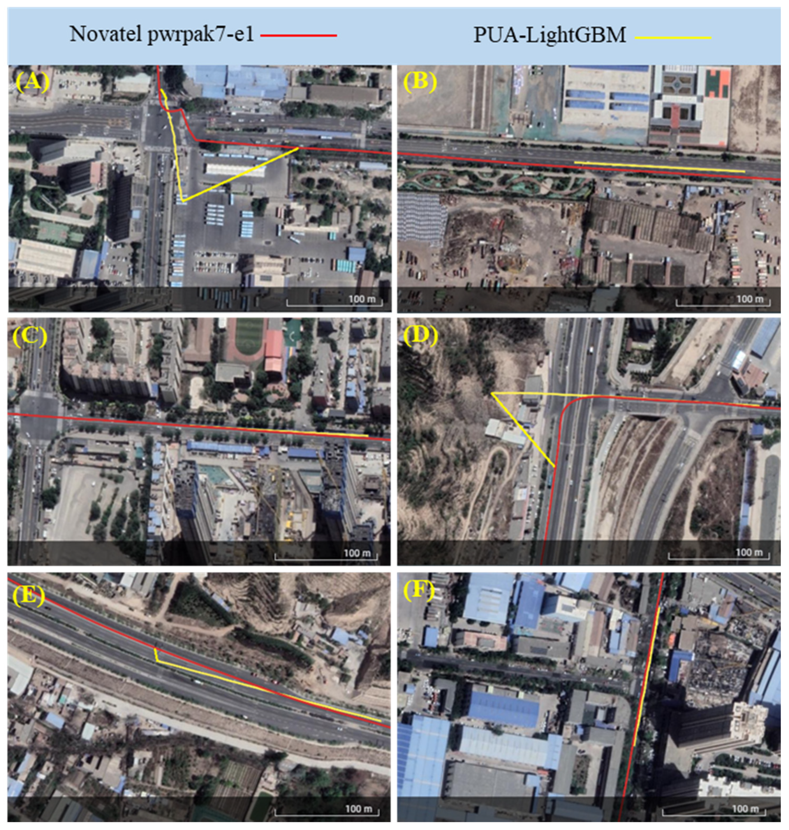
4.2. The Field Test Analysis

Figure 4 shows the vehicle trajectories outputted by PUA-LightGBM (in yellow) and Novatel pwrpak7-e1 (in red) on the six road segments of the field test. The trajectory output from PUA-LightGBM is the model-predicted trajectory, and the Novatel pwrpak7-e1 integrated navigation system provides the trajectory as the vehicle reference trajectory. As can be seen from the trajectory figure, the PUA-LightGBM model predicted the position changes of vehicles on straight roads (Figure 4B,C,E,F) better than those of vehicles on curved road (Figure 4A,D). This is in line with the analysis by Chiang and Huang, which found that the results predicted by the position prediction model during U-turns or sharp turns (where there are significant dynamic changes in the vehicle’s movement) produce significant position errors [13]. The vehicle motion is more stable when travelling on a straight road, and the PUA-LightGBM model is better at predicting position changes. However, the two turning segments chosen for the experiments were both sharp turning segments, where the vehicle experienced significant dynamic changes in motion and vibration of the vehicle body. The INS data at this point did not accurately reflect the vehicle’s turning state, and the model’s training set did not contain enough vehicle turning situations, causing the PUA-LightGBM model to be less effective in predicting the position change of the vehicle when driving around a turn.

Table 3. Average absolute positional error for the PUA-LightGBM model and the PUA-RandomForest model.

Outage Road Segment	Road Length (m)	Average Absolute Positional Error (m)		Percentage Improvement (%)
		PUA-RandomForest	PUA-LightGBM
a	191.18	61.85	59.71	+3.5
b	222.58	22.11	21.90	+0.95
c	215.24	17.43	17.55	−0.69
d	246.46	32.84	33.52	−2.1
e	231.65	23.33	24.48	−4.9
f	146.88	22.03	21.92	+0.50

shows the average absolute error between the predicted and true positions of the PUA-LightGBM and PUA-RandomForest models for the GNSS outage scenario. PUA-LightGBM outperformed PUA-RandomForest on road segments a, b, and f in terms of position prediction. On road segments c, d, and e, the position prediction accuracy of PUA-LightGBM was slightly lower than that of PUA-RandomForest. Overall, the prediction error of PUA-LightGBM was less different from PUA-RandomForest. The PUA-LightGBM model, on the other hand, had a much shorter training time than the PUA-RandomForest model (Table 2). This suggests that PUA-LightGBM is more efficient in training, costs less, and has the potential for dynamic updating. The model does not need to be trained in advance and can be dynamically trained or updated while the vehicle is moving. This provides some flexibility to the PUA-LightGBM model and allows it to predict vehicle position changes on a variety of complex road segments via dynamic updating of the model.

5. Conclusions

This paper proposes a prediction model of vehicle position change in the event of a GNSS outage based on position update architecture using LightGBM. The model solves the problem of data accuracy degradation of the GNSS/INS integrated navigation system for a vehicle when the satellite signal quality is weak or there is a GNSS outage and improves the existing AI-based GNSS/INS integrated navigation algorithm. When the vehicle is capable of receiving available GNSS signals, on-board INS and GNSS data are collected, and the PUA-LightGBM model is trained. In the event of a GNSS outage, INS data are used as the input to PUA-LightGBM to obtain the changes in longitude and latitude between the two epochs output by the model, thus predicting the vehicle’s position at this time. Experiments on six road segments were conducted using a self-designed vehicle navigation data acquisition system. The results show that the error in predicting vehicle position in the event of a GNSS outage for PUA-LightGBM is less than that of PUA-RandomForest. However, the time required to train the PUA-LightGBM model is only 3.076 s, which is significantly less than the time required to train the PUA-RandomForest model. The authors believe that two factors should be considered in future research to enhance the predictive model’s effectiveness in the event of a GNSS outage. One is reducing the noise in INS data to obtain better position predictions. The other is the higher training efficiency of PUA-LightGBM, which can save time and enable the model to be dynamically trained or updated during vehicle operation. Thus, the PUA-LightGBM can adapt to the prediction of vehicle position change on various complex road segments. The limitation of this study is that the validation of the PUA-LightGBM model was not real-time. It might be better to develop a real vehicle navigation system for embedding the PUA-LightGBM model in the future.

References

1. Vörös, F.; Gartner, G.; Peterson, M.P.; Kovács, B. What Does the Ideal Built-In Car Navigation System Look Like?—An Investigation in the Central European Region. Appl. Sci. 2022, 12, 3716. [Google Scholar] [CrossRef]
2. Onyekpe, U.; Palade, V.; Kanarachos, S. Learning to localise automated vehicles in challenging environments using Inertial Navigation Systems (INS). Appl. Sci. 2021, 11, 1270. [Google Scholar] [CrossRef]
3. Angrisano, A. GNSS/INS Integration Methods. Ph.D. Thesis, Universita’degli Studi di Napoli Parthenope, Naple, Italy, 2010; p. 21. [Google Scholar]
4. Liu, H.; Nassar, S.; El-Sheimy, N. Two-filter smoothing for accurate INS/GPS land-vehicle navigation in urban centers. IEEE Trans. Veh. Technol. 2010, 59, 4256–4267. [Google Scholar] [CrossRef]
5. Yang, L.; Li, Y.; Wu, Y.; Rizos, C. An enhanced MEMS-INS/GNSS integrated system with fault detection and exclusion capability for land vehicle navigation in urban areas. GPS Solut. 2014, 18, 593–603. [Google Scholar] [CrossRef]
6. Sasani, S.; Asgari, J.; Amiri-Simkooei, A. Improving MEMS-IMU/GPS integrated systems for land vehicle navigation applications. GPS Solut. 2016, 20, 89–100. [Google Scholar] [CrossRef]
7. Wang, M.; Wu, W.; He, X.; Li, Y.; Pan, X. Consistent ST-EKF for long distance land vehicle navigation based on SINS/OD integration. IEEE Trans. Veh. Technol. 2019, 68, 10525–10534. [Google Scholar] [CrossRef]
8. Cui, B.; Wei, X.; Chen, X.; Li, J.; Li, L. On sigma-point update of cubature Kalman filter for GNSS/INS under GNSS-challenged environment. IEEE Trans. Veh. Technol. 2019, 68, 8671–8682. [Google Scholar] [CrossRef]
9. Bijjahalli, S.; Sabatini, R. A high-integrity and low-cost navigation system for autonomous vehicles. IEEE Trans. Intell. Transp. Syst. 2019, 22, 356–369. [Google Scholar] [CrossRef]
10. Chiang, K.-W.; Noureldin, A.; El-Sheimy, N. Multisensor integration using neuron computing for land-vehicle navigation. GPS Solut. 2003, 6, 209–218. [Google Scholar] [CrossRef]
11. Aggarwal, P.; Bhatt, D.; Devabhaktuni, V.; Bhattacharya, P. Dempster Shafer neural network algorithm for land vehicle navigation application. Inf. Sci. 2013, 253, 26–33. [Google Scholar] [CrossRef]
12. Noureldin, A.; Karamat, T.B.; Eberts, M.D.; El-Shafie, A. Performance enhancement of MEMS-based INS/GPS integration for low-cost navigation applications. IEEE Trans. Veh. Technol. 2008, 58, 1077–1096. [Google Scholar] [CrossRef]
13. Chiang, K.-W.; Huang, Y.-W. An intelligent navigator for seamless INS/GPS integrated land vehicle navigation applications. Appl. Soft Comput. 2008, 8, 722–733. [Google Scholar] [CrossRef]
14. Yue, S.; Cong, L.; Qin, H.; Li, B.; Yao, J. A robust fusion methodology for MEMS-based land vehicle navigation in GNSS-challenged environments. IEEE Access 2020, 8, 44087–44099. [Google Scholar] [CrossRef]
15. Liu, Y.; Luo, Q.; Zhou, Y. Deep Learning-Enabled Fusion to Bridge GPS Outages for INS/GPS Integrated Navigation. IEEE Sens. J. 2022, 22, 8974–8985. [Google Scholar] [CrossRef]
16. Khankalantary, S.; Rafatnia, S.; Mohammadkhani, H. An adaptive constrained type-2 fuzzy Hammerstein neural network data fusion scheme for low-cost SINS/GNSS navigation system. Appl. Soft Comput. 2020, 86, 105917. [Google Scholar] [CrossRef]
17. Ke, G.; Meng, Q.; Finley, T.; Wang, T.; Chen, W.; Ma, W.; Ye, Q.; Liu, T.-Y. Lightgbm: A highly efficient gradient boosting decision tree. In Proceedings of the Advances in Neural Information Processing Systems 30 (NIPS 2017), Long Beach, CA, USA, 4–9 December 2017; Volume 30. [Google Scholar]
18. El-Sheimy, N.; Chiang, K.-W.; Noureldin, A. The utilization of artificial neural networks for multisensor system integration in navigation and positioning instruments. IEEE Trans. Instrum. Meas. 2006, 55, 1606–1615. [Google Scholar] [CrossRef]
19. Adusumilli, S.; Bhatt, D.; Wang, H.; Bhattacharya, P.; Devabhaktuni, V. A low-cost INS/GPS integration methodology based on random forest regression. Expert Syst. Appl. 2013, 40, 4653–4659. [Google Scholar] [CrossRef]
20. Bhatt, D.; Aggarwal, P.; Devabhaktuni, V.; Bhattacharya, P. A novel hybrid fusion algorithm to bridge the period of GPS outages using low-cost INS. Expert Syst. Appl. 2014, 41, 2166–2173. [Google Scholar] [CrossRef]
21. Liang, W.; Luo, S.; Zhao, G.; Wu, H. Predicting hard rock pillar stability using GBDT, XGBoost, and LightGBM algorithms. Mathematics 2020, 8, 765. [Google Scholar] [CrossRef]
22. Chen, C.; Zhang, Q.; Ma, Q.; Yu, B. LightGBM-PPI: Predicting protein-protein interactions through LightGBM with multi-information fusion. Chemom. Intell. Lab. Syst. 2019, 191, 54–64. [Google Scholar] [CrossRef]
23. Ju, Y.; Sun, G.; Chen, Q.; Zhang, M.; Zhu, H.; Rehman, M.U. A model combining convolutional neural network and LightGBM algorithm for ultra-short-term wind power forecasting. IEEE Access 2019, 7, 28309–28318. [Google Scholar] [CrossRef]
Figure 1. PUA-based LightGBM machine learning model. (A) Position update architecture (PUA), t—time; VINS(t)—Velocity provided by INS at t; θINS(t)—Heading angle provided by INS at t; δNPUA(t)—Latitude difference between epoch t and epoch t − 1; δEPUA(t)—Longitude difference between epoch t and epoch t − 1; (B) Scheme of the LightGBM machine learning model based on the PUA.
Applsci 12 05565 g001
Figure 2. Experimental device and method. (A) Two integrated navigation systems, 1—1st antennae; 2—2nd antennae; 3—3rd antennae; (B) closed-loop experimental road trajectory.
Applsci 12 05565 g002
Figure 3. Training process of PUA-LightGBM model and histogram-based decision tree algorithm. DT—Regression Decision Tree; f i ( x )—Output of DTi; i = 1 n f i ( x ) —final output of the PUA-LightGBM model.
Applsci 12 05565 g003
Figure 4. The vehicle trajectories outputted by PUA-LightGBM (in yellow) and Novatel pwrpak7-e1 (in red) on six road segments of the field test. (A) Turn and downslope road, (B) straight and level road, (C) straight and upslope road, (D) turn and upslope road, (E) straight and level road, (F) straight and downslope road.
Applsci 12 05565 g004