Article

Synchronization Sliding Mode Control of Closed-Kinematic Chain Robot Manipulators with Time-Delay Estimation

1
Department of Electrical Engineering and Computer Science, School of Engineering, The Catholic University of America, 620 Michigan NE Ave., Washington, DC 20064, USA
2
Automatic Control Department, Ho Chi Minh City University of Technology and Education, Ho Chi Minh City 700000, Vietnam
*
Author to whom correspondence should be addressed.
Appl. Sci. 2022, 12(11), 5527; https://doi.org/10.3390/app12115527
Submission received: 4 May 2022 / Revised: 26 May 2022 / Accepted: 27 May 2022 / Published: 29 May 2022
(This article belongs to the Special Issue Modelling and Control of Mechatronic and Robotic Systems, Volume II)

Abstract

:
Control of closed-kinematic chain manipulators (CKCM) with uncertain dynamics is a tremendous challenge due to the synchronization among actual joints and end-effectors, limited workspace, and nonexistent closed-form solutions of forward kinematics. This paper proposes a synchronization control scheme based on the concept of sliding mode control (SMC) developed for CKCMs called nonsingular fast terminal sliding mode control (NFTSMC) in conjunction with the time-delay estimation (TDE) method to address the above issues. First, the cross-coupling error is derived by combining position errors and synchronization errors to achieve the synchronization goal and then used to form a sliding mode surface of the NFTSMC. After that, a control law is developed based on the sliding mode surface to ensure faster asymptotic convergence of the errors of both position and synchronization of the CKCMs in a finite and minimal time. Then, the TDE control scheme with no prior knowledge of manipulator dynamics is employed to estimate the unknown dynamics and disturbances and thereby reject the effects of chattering caused by the NFTSMC. Lyapunov stability theorem is employed to show that the overall system controlled by the proposed control scheme achieves asymptotic convergence of errors and system stability. The performance of the proposed control is assessed by computer simulation on a 2 degrees-of-freedom (DOF) planar CKCM manipulator and simulation results are presented and discussed.

1. Introduction

Closed-kinematic chain manipulators (CKCMs) for which its motion is achieved in all degrees-of-freedom (DOF) by the combined motion of their active joints can provide higher positioning accuracy and greater payload handling capability than the conventional open-kinematic chain manipulators (OKCM) composed of serial linkages or rigid bodies [1,2,3,4]. Despite the above advantages, CKCMs possess several drawbacks such as synchronization among actual joints and end-effectors, limited workspace, and nonexistent closed-form solutions of forward kinematics. To address the above issues, the concept of synchronization control has been considered, and as a result, there has been much effort in the development and implementation of error synchronization-based control schemes for CKCMs. In a synchronization-based control scheme, all joints are synchronously driven to improve CKCM’s performance.
The synchronization concept was first introduced in [5], and it was applied to perform tracking control of parallel robots [6,7,8,9]. Most existing synchronized control schemes are model-based such as the computed torque control (CTC) [10], adaptive control [11,12], and sliding mode control (SMC) [13,14]. In general, a SMC scheme consists of a driving component that forces the system’s trajectory to reach a stable hyperplane (sliding surface) and a design of a sliding surface that assures the plant’s desired error dynamics. The implementation of the above synchronized control schemes requires a precise dynamical model of the manipulator, for which its calculation is highly computationally intensive. Moreover, it was concluded that an accurate mathematical dynamic model of CKCMs is difficult to obtain. Consequently, the above model-based control schemes are not suitable for real-time control of CKCM manipulators, particularly those with more than 2 DOFs. To tackle the above dynamic modeling issue, the authors in [15,16] considered synchronized control schemes that have simple structures and do not require knowledge of the manipulator dynamics to implement their control laws. However, those control approaches proposed for parallel manipulators can only achieve asymptotic stability, which requires infinite time to converge to an equilibrium point. In order to assure finite-time convergence, the terminal SMC (TSMC) scheme was proposed in [17,18,19]. Then, the advantage control scheme of TSMC, called Nonsingular Fast Terminal Sliding Mode Control (NFTSMC), was introduced in [20,21]. This developed control scheme can handle the singularity and fast convergence of the system. Recently, the NFTSMC was combined with synchronization, and this control scheme was applied to a parallel robot manipulator in [7]. It used the cross-coupling error that combined both tracking errors among the active joints and synchronization errors of a parallel robot to fix the actuator’s external disturbances and dynamic uncertainties. Thus, the tracking performance of the robot improved significantly. However, the gains of this control scheme are still selected based on conservative estimates of the dynamic manipulator model. Thus, it leads to complications in the highly complicated model in calculations.
Recently, a simple model-free controller called Time-Delay Estimation (TDE) was applied to CKCMs to solve the above issue. The TDE has been employed to control robot manipulators over the last decade because of its efficient computation capability [22,23,24]. It used time-delayed information to estimate unknown dynamics and disturbances in a sufficiently small time-delay. Lately, the TDE has been combined with Nonsingular Terminal Sliding Mode (NTSM) control [25] to provide highly robust and precise control schemes for robots with a fast convergence finite time. To our best knowledge, control schemes combining the TDE, the NFTSMC and synchronization have not been considered for controlling CKCMs.
Based on the above analysis, a simple model-free synchronization control system for CKCMs based on TDE and NFTSMC is proposed in this paper to pursue simplicity while preserving the robustness of CKCMs.
Comparing to the existing control schemes approach for robot manipulators, the contribution of this paper can be marked as the following significant points:
(1)
Unlike the above-mentioned control schemes, the proposed control scheme TDE-based NFTSMC with synchronization is proposed for the first time.
(2)
A new control scheme is proposed based on the combination of TDE-based NFTSMC and synchronization control.
(3)
The proposed control scheme is to optimally synchronize the robot joints to minimize the synchronization errors with a NFTSMC-based controller while the robot dynamics and disturbances are estimated and compensated by a TDE-based subsystem.
This paper presents the computer simulation studies of the performance of the proposed control scheme using Matlab-Simulink. Comparative studies with other existing control schemes will be conducted.
The paper is organized as follows. Section 2 presents the structure of the proposed control scheme. Section 3 presents the control scheme analysis without TDE while Section 4 presents the description of subsystems and discusses their simplicity and efficiency. The stability and the stability provided by the control scheme is analyzed and discussed in Section 5. Section 6 presents and discusses results of computer simulation conducted to study the performance of the control scheme applied to control the motion of a 2 DOF CKCM manipulator in comparison with other existing control schemes. Finally, Section 7 concludes the paper with a summary of the paper and final comments.

2. Structure of the Control Scheme

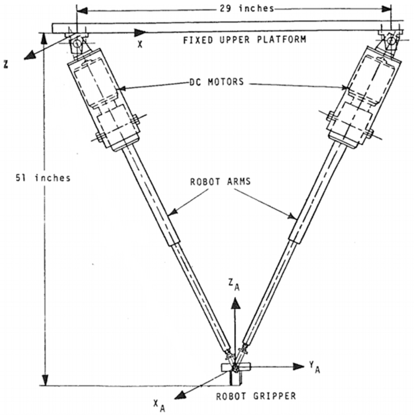
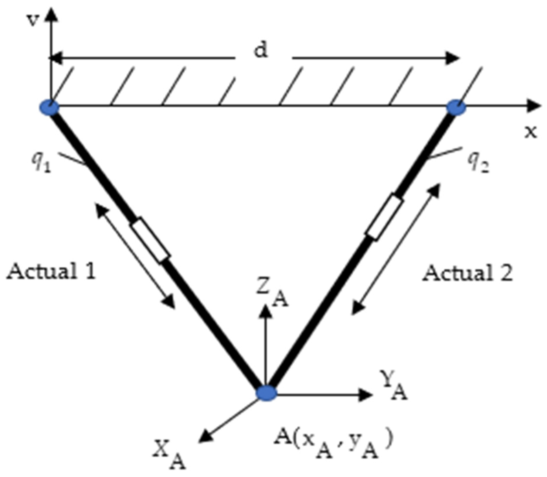
2.1. Kinematic Scheme of the CKCM

The structures of the 2 DOF CKCM manipulator and the frame assignment are shown in Figure 1 and Figure 2, respectively. Figure 1 shows a two DOF CKCM manipulator, which is a special case of the n-DOF CKCM manipulator. It consists of an end-effector platform and a fixed upper platform interconnected by two links. All links act in a parallel manner and share the same payload.
Figure 2 depicts the frame assignment for the two DOF planar CKCM manipulator with a two-dimensional coordinate system (x, y). From this figure, we obtain the following:
q 1 2 = x 2 + y 2
q 2 2 = ( d x ) 2 + y 2
where d is the distance between the pin joints hanging the two actuators, (x, y) represents the Cartesian position of the end-effector, and q 2 and q 2 are the length of the first and second legs, respectively.
We see that (1) and (2) represent a closed-form solution for the inverse kinematics in the sense that they can be used to determine the leg lengths q 1 and q 2 that yield a desired Cartesian position (x, y).
Moreover, from (1) and (2), the Cartesian variables x and y can be obtained as follows.
x = q 1 2 q 2 2 + d 2 2 d
y = 4 d 2 q 1 2 ( q 1 2 q 2 2 + d 2 ) 2 d
We see that (3) and (4) represent a closed-form solution for the forward kinematics in the sense that a Cartesian position can be determined based the actual leg lengths q 1 and q 2 . We note that, due to the small number of DOFs of this manipulator, it has closed-form solutions for both its forward and inverse kinematics.

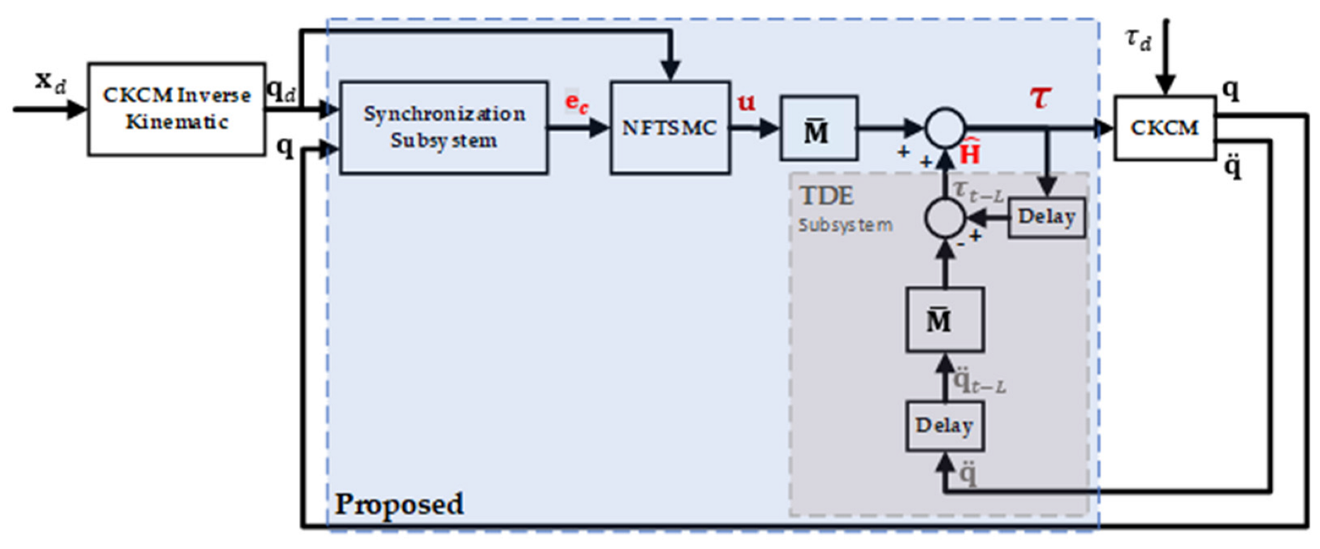
2.2. Structure of the Proposed Control Scheme

The structure of the proposed control scheme is presented in Figure 2. It mainly consists of three subsystems: the Synchronization Subsystem, the NFTSMC Subsystem. and the TDE Subsystem.
The notations used in Figure 3 are listed below:
  • x d R n : the desired Cartesian configuration vector. (Note: Configuration means both position and orientation of the CKCM);
  • q d R n , q R n and q ¨ R n : the desired joint vector, actual joint vector, and actual acceleration vector, of the CKCM, respectively;
  • e c R n : the synchronization error vector;
  • u R n : the control law vector of the NFTSMC;
  • M ¯ ( q ) R n × n : constant, diagonal matrix selected by the TDE;
  • r R n : the output vector of the NFTSMC Subsystem;
  • τ R n : the compensated control input vector to the CKCM;
  • τ d R n : the external disturbances vector;
  • L: the estimate time delay of the TDE;
  • q ¨ t L R n and τ t L R n : the past acceleration vector and past control input vector of the CKCM, respectively;
  • H ^ R n : the estimate of all nonlinear terms including the inertia uncertainty, Coriolis/centripetal vector, gravitational vector, friction vector, and disturbances.
The operation of the proposed control scheme applied to control the motion of an n-DOF CKCM is described as follows. The desired Cartesian vector x d of the manipulator configuration (position and orientation) specified by the user or obtained by a trajectory planner is transformed to its corresponding desired joint vector q d by the CKCM Inverse Kinematic Transformation. The desired joint vector q d and the actual joint vector q (provided by the CKCM joint sensors) are supplied to the Synchronization Subsystem, which then produces the position errors e i = q d i q i of every ith active joint, the synchronization error e S , and the cross-coupling error e c between the active joints. The cross-coupling error e c is then inputted to the NFTSMC subsystem that in turn based on e c defines a sliding surface to achieve the above desired behavior of the errors. Next, the control law u composed based on the sliding surface will be a driving component forcing the system’s trajectory to reach a stable hyperplane (sliding surface). This control law u will then serve as part of the input τ to the CKCM and is developed to ensure asymptotic convergence of the errors of both position and synchronization of the CKCM in a finite and minimal time. The TDE subsystem uses the past control input and acceleration of the CKCM to estimate the CKCM dynamics and the disturbance torques, which are required for the implementation of the input τ to CKCM.

3. Control Scheme Analysis without TDE

The dynamics of an n-DOF CKCM manipulator can be represented in joint-space as follows [25]:
M ( q ) q ¨ + C ( q , q ˙ ) q ˙ + G ( q ) + F ( q , q ˙ ) + τ d = τ
where M ( q ) R n × n stands for the generalized inertia matrix, C ( q , q ˙ ) R n × n is the Coriolis/centripetal matrix, G ( q ) R n is the gravitational vector, and F ( q , q ˙ ) R n is the friction forces.
Suppose system (5) can be decomposed into n decoupled systems and is presented by the following:
M ¯ q ¨ + H ( q , q ˙ , q ¨ ) = τ
where M ¯ is a constant diagonal matrix, and H ( q , q ˙ , q ¨ ) represents the necessary CKCM dynamics and the disturbance torques. Then, from (5) and (6), we obtain the following.
H ( q , q ˙ , q ¨ ) = [ M ( q ) M ¯ ] q ¨ + C ( q , q ˙ ) q ˙ + G ( q ) + F ( q , q ˙ ) + τ d
Now we apply an input τ such that the following is the case.
τ = M ¯ u + H ( q , q ˙ , q ¨ )
In order to implement (8), the control system must evaluate H ( q , q ˙ , q ¨ ) which in light of (7) requires heavy computation and thereby making the proposed control scheme impractical and not suitable for real-time control applications. Consequently, some computationally efficient estimation of H ( q , q ˙ , q ¨ ) is needed for the control scheme, which the TDE Subsystem could provide. Finally, the Synchronization Subsystem will enhance the overall performance of the control system by using the synchronization errors instead of the conventional joint errors. Detailed development of the above subsystems will be presented below.

4. Description of Subsystems

This section presents the function of the three subsystems of the control structure including the Synchronization Subsystem, the NFTSMC Subsystem, and the TDE Subsystem.

4.1. The Synchronization Subsystem

In this section, the error equations will be developed to achieve the synchronization goal. First the trajectory tracking error e i of the ith active joint is defined as follows:
e i ( t ) = q d i ( t ) q i ( t )
where q d i ( t ) and q i ( t ) denote the desired and actual trajectories of the ith active joint, respectively.
Then, the tracking error vector e ( t ) can be written as follows.
e ( t ) = [ e 1 ( t )   e 2 ( t ) e n ( t ) ] T
The synchronization goal is to make the tracking errors of all active joints identical at all times, which can be achieved if the following is the case.
e 1 ( t ) = e 2 ( t ) = e n ( t )
In order for (11) to be valid, a control scheme must be aware of all the joint errors and must control the motions of all joints, thereby resulting into possible control and communication errors and heavy real-time computational requirements. Alternatively, (11) can be satisfied by achieving its following sub-goals [8]:
e s 1 ( t ) = 2 e 1 ( t ) [ e 2 ( t ) + e n ( t ) ] e s i ( t ) = 2 e i ( t ) [ e i + 1 ( t ) + e i 1 ( t ) ] e s n ( t ) = 2 e n ( t ) [ e n 1 ( t ) + e 1 ( t ) ]
where e s i ( t ) presents the synchronization errors of the ith active joint.
It is evident that if all synchronization errors in (12) are equal to zero, then the original synchronization goal stated in (11) is automatically achieved.
From (12), a synchronization error vector e s can be written as follows:
e s ( t ) = 2 1 0 1 1 2 1 0 0 1 2 1 1 0 1 2 e 1 ( t ) e 2 ( t ) e n 1 ( t ) e n ( t ) = C e ( t )
where C is the synchronization transformation matrix and e s ( t ) = [ e s 1 ( t ) e s 2 ( t ) e s 3 ( t ) e s n ( t ) ] T . The cross-coupling error vector that combines both tracking errors and synchronization errors is defined as follows:
e c ( t ) = e ( t ) + α e s ( t ) = ( I + α C ) e ( t )
where I is the n × n identity matrix, and α is an n × n diagonal positive definite matrix. Since every leading principal sub-matrix of ( I + α C ) has positive determinant, ( I + α C ) is positive definite. [26]
Remark 1.
Assuming that all the elements of matrix α are very small, then if e c ( t ) is controlled such that as t , e c ( t ) 0 then e ( t ) 0 and then e s ( t ) 0 and finally e i ( t ) = e i + 1 ( t ) (synchronization goal).

4.2. The NFTSMC and TDE Subsystems

This section presents the development of the control law of the NFTSMC Subsystem in conjunction with the TDE Subsystem.

4.2.1. Preliminaries and Notations

The preliminaries and notations can be stated as follow
x [ c ] = | x | c sign ( x ) ,   where   c > 0
It can be easily verified that as c 1 , the following is the case.
d d t x [ c ] = c | x | c 1 x ˙
The sign function is defined as follows.
sign ( x ) = { 1 if   x > 0 0 if   x = 0 1 if   x < 0
The power of error vectors is defined as follows.
e [ φ ] : = ( e 1 [ φ ] , , e n [ φ ] ) T R n e ˙ [ φ ] : = ( e 1 [ φ ] , , e ˙ 1 [ φ ] ) T R n | e | φ 1 : = d i a g ( | e 1 | φ 1 , , | e n | φ 1 ) R n × n | e ˙ | φ 1 : = d i a g ( | e ˙ 1 | φ 1 , , | e ˙ n | φ 1 ) R n × n
The spectral norm A of a matrix A R n × m is defined as A = λ max { A T A } where λ max { A T A } is the biggest eigenvalue of A T A .

4.2.2. The NFTSMC and TDE Sybstems Design

First a nonsingular terminal sliding surface is defined as [20,27].
s = e c + K 1 e c p 1 / q 1 + K 2 e ˙ c p 2 / q 2
where K 1 and K 2 are diagonal design matrices, 1 < p 1 / q 1 < 2 , 1 < p2/q2 < 2, and p 1 , p 2 , q 1 , and q 2 are positive odd integers.
As discussed above, the implementation of (8) requires the computation of H ( q , q ˙ , q ¨ ) , which is in light of (7) highly computationally intensive. Thus, an estimate of H ( q , q ˙ , q ¨ ) is needed. We assume that L is the smallest obtainable time between which H ( q , q ˙ , q ¨ ) remains almost unchanged, such that an estimate of H ( q , q ˙ , q ¨ ) , namely H ^ ( q , q ˙ , q ¨ ) is equal to H ( q , q ˙ , q ¨ ) t L which is H ( q , q ˙ , q ¨ ) evaluated at (t−L). In other words, we obtain [22] the following:
H ^ ( q , q ˙ , q ¨ ) = H ( q , q ˙ , q ¨ ) t L
where q ¨ t L can be computed as follows.
q ¨ t L = q t q t L L q t L q t 2 L L L = ( q t 2 q t L + q t 2 L ) L 2
From (6) and (16), we obtain the following.
H ^ ( q , q ˙ , q ¨ ) = τ t L M ¯ q ¨ t L
Consequently, (8) can be expressed as follows.
τ = H ^ ( q , q ˙ , q ¨ ) + M ¯ u
We proceed to develop a control u as follows.
u = q ¨ d + q 2 p 2 [ K 2 ( I + α C ) ] 1 [ | e ˙ c | p 2 / q 2 1 ] 1 ( 1 + p 1 q 1 K 1 | e c | p 1 / q 1 1 ) e ˙ c + K s + K s w sign ( s )
where K and K s w are diagonal design matrices, sign ( s ) = ( sign ( s 1 ) , , sign ( s n ) ) T R n . x d R n .
Thus, replacing u in (19) by (20) and using (18), we obtain the following.
τ = ( τ t L M ¯ q ¨ t L ) TDE + M ¯ [ q ¨ d + q 2 p 2 [ K 2 ( I + α C ) ] 1 [ | e ˙ c | p 2 / q 2 1 ] 1 ( 1 + p 1 q 1 K 1 | e c | p 1 / q 1 1 ) e ˙ c + K s + K s w sign ( s ) ] NFTSM   control
As indicated above in Equation (21), CKCM input τ consists of two main components: a TDE-based input and an NFTSM input. The TDE-based component minimizes the impact of the unknown CKCM dynamics while the NFTSM component forces the cross-coupling errors e c and tracking error e to converge to zero asymptotically. Furthermore, in light of the application of the TDE Subsystem as presented above and reflected in Figure 1, the TDE-based component can be derived with the estimate H ^ ( q , q ˙ , q ¨ ) of H ( q , q ˙ , q ¨ ) using (16), instead of having to compute H ( q , q ˙ , q ¨ ) directly, thereby making the control scheme highly efficient.

5. Stability Analysis

This section presents the stability analysis of the control scheme using the Lyapunov Theorem. Substituting τ   in (6) by (21), using (9) and (14) and solving for e ¨ c , after rearranging some terms, we obtain the following:
e ¨ c = { q 2 p 2 [ K 2 ] 1 [ | e ˙ c | p 2 / q 2 1 ] 1 ( 1 + p 1 q 1 K 1 | e c | p 1 / q 1 1 ) e ˙ c + ( I + α C ) [ K s + K s w sign ( s ) ] } + ( I + α C ) ε
where the TDE error ε is defined as follows.
ε = M ¯ 1 [ H ( q , q ˙ , q ¨ ) H ^ ( q , q ˙ , q ¨ ) ]
Using (15), s ˙ can be obtained as follows.
s ˙ = e ˙ c + p 1 q 1 K 1 | e c | p 1 / q 1 1 e ˙ c + p 2 q 2 K 2 | e ˙ c | p 2 / q 2 1 e ¨ c
Next, we consider a candidate Lyapunov function V = s T s 2 . Using (24), the derivative of V with respect to time is obtained as follows.
V ˙ = s T s ˙ = s T [ e ˙ c + p 1 q 1 K 1 | e c | p 1 / q 1 1 e ˙ c + p 2 q 2 K 2 | e ˙ c | p 2 / q 2 1 e ¨ c ]
Applying (24) in (25) provides the following.
V ˙ = s T { p 2 q 2 ( I + α C ) K 2 | e ˙ c | p 1 / q 1 1 [ K s K s w sign ( s ) + ε ] }
In other to achieve the asymptotic stability of s ˙ about the equilibrium point s = 0 , the following conditions must be satisfied [28]:
(a)
V ˙ < 0   for   s 0 ;
(b)
lim | s | V = .
Condition (b) is obviously satisfied by V. In (26), since p 2 and q 2 are positive integers and 1 < p 2 / q 2 < 2 , there is | e ˙ c i | p 2 / q 2 1 > 0   for   e ˙ c i 0 [29].
Thus, (26) can be presented as follows.
V ˙ = s T { p 2 q 2 ( I + α C ) K 2 | e ˙ c | p 1 / q 1 1 [ K s K s w sign ( s ) + ε ] } s T [ K s K s w sign ( s ) + ε ]
The derivative of the candidate Lyapunov function (27) is negative definite if the following is the case:
{ K s w } i i > | ε i |
where i i denotes ith diagonal element of .
Thus, if ε is bounded, the stability condition (28) ensures that the time derivative of the candidate Lyapunov function is negative and the cross-coupling error is bounded.
Using (19), (6) becomes the following.
H ( q , q ˙ , q ¨ ) H ^ ( q , q ˙ , q ¨ ) = M ¯ ( u q ¨ )
Applying (29), the TDE error in (23) is given as follows.
ε = u q ¨
From (5), the acceleration q ¨ can be determined as follows.
q ¨ = M 1 ( q ) [ τ C ( q , q ˙ ) q ˙ G ( q ) F ( q , q ˙ ) τ d ]
Substituting (31) into (30) yields the following.
M ε = M u + ( C ( q , q ˙ ) q ˙ + G ( q ) + F ( q , q ˙ ) + τ d τ )
Then, using (16) and (19), (32) becomes the following.
M ε = M u + ( C ( q , q ˙ ) q ˙ + G ( q ) + F ( q , q ˙ ) + τ d M ¯ u H ( q , q ˙ , q ¨ ) t L )
From (7), the delayed nonlinear term can be derived as follows.
H ( q , q ˙ , q ¨ ) t L = ( M t L M ¯ ) q ¨ t L + ( C ( q , q ˙ ) q ˙ ) t L + ( G ( q ) ) t L + ( F ( q , q ˙ ) ) t L + ( τ d ) t L
Substituting (34) into (33) provides the following:
M ε = ( M M ¯ ) u ( M t L M ¯ ) q ¨ t L + Ω
where the following is the case.
Ω = C ( q , q ˙ ) q ˙ + G ( q ) + F ( q , q ˙ ) + τ d ( C ( q , q ˙ ) q ˙ ) t L ( G ( q ) ) t L ( F ( q , q ˙ ) ) t L ( τ d ) t L
The friction term F in (36) can be divided as F = F V + F C , where F V denotes that the viscous friction is continuous, and F C denotes that the Coulomb friction is bounded and discontinuous at velocity reversal [25]. Next, we divide Ω into continuous term and discontinuous term to obtain the following:
Ω Ω con + Ω discon
where the following is the case.
Ω con C ( q , q ˙ ) q ˙ + G ( q ) + F V + τ d ( C ( q , q ˙ ) q ˙ ) t L ( G ( q ) ) t L ( F ( q , q ˙ ) ) t L ( τ d ) t L Ω discon F C ( F C ) t L }
If C ( q , q ˙ ) q ˙ + G ( q ) + F V + τ d is continuous and bounded, then Ω con = O ( L 2 ) , where O is used to describe the error term in an approximation to a mathematical function [30].
In addition, the discontinuous term Ω discon is described as follows.
Ω discon { b ,   at   velocity   reversal 0 ,   otherwise .
Thus, Ω is bounded by the following:
Ω b + O ( L 2 )
for a sufficient small L, where b is a constant vector. The approximation error can be made small by reducing sampling time L.
From (30), the delayed nonlinear term is given by the following.
q ¨ t L = u t L ε t L
Substituting (41) to (35) yields the following
M ε = [ ( M M ¯ ) u ( M M ¯ ) q ¨ t L + ( M M t L ) q ¨ t L + Ω ] = ( M M ¯ ) ε t L + [ ( M M ¯ ) ( u u t L ) + ( M M t L ) q ¨ t L + Ω ]
Therefore, from (42), ε can be determined as follows:
ε = E ε t L + E μ 1 + μ 2
where the following is the case.
E = I M 1 M ¯ ,   μ 1 = u u t L ,   μ 2 = M 1 [ ( M M t L ) q ¨ t L + Ω ]
For a sufficiently small-time delay L, μ 1 and μ 2 are bounded.
There is a conformal mapping on the complex plane from continuous-time to discrete-time [31]. In the discrete time domain, (43) is represented as follows.
ε ( k ) = E ( k ) ε ( k 1 ) + E ( k ) μ 1 ( k ) + μ 2 ( k )
We assume E < 1 by properly selecting M ¯ [31]. Thus, the eigenvalues of E ( k ) reside inside a unit circle [32]. As a result, (45) is asymptotically bounded with bounded function μ 1 and μ 2 . Therefore, E < 1 implies the boundness of the ε in (43).
When ε is bounded, then (28) is satisfied and as a result, the candidate Lyapunov function (27) is negative definite. Thus, this assures of the boundedness of the cross-coupling error. Furthermore, when the cross-coupling error is bounded, the tracking error is bounded. Consequently, all the above errors and the TDE error ε will never grow out of bound and the system is uniformly stable.

6. Computer Simulation Study

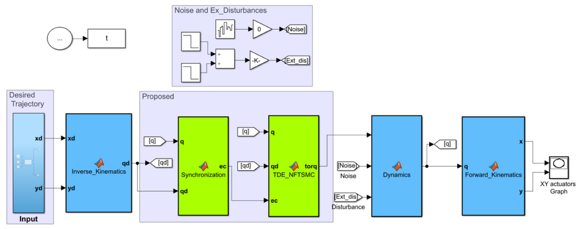
6.1. Simulation Setup

The proposed scheme can be applied for a general n DOF CKCM manipulator. However, the implementation and application for a n DOF manipulator require massive computation effort and hardware complexity. Therefore, a 2 DOF CKCM robot manipulator that resembles a special case of the complete n DOF manipulation was designed and built for the purpose of testing of the results obtained in our projects. Hence, this article is devoted to investigate the simulation study of the obtained results on the 2 DOF manipulator.
In this section, computer simulation will be conducted to study the performance of the above NFTSMC in comparison to other existing control schemes when they are employed to control the motion of a 2-DOF CKCM.
The computer simulation study for the NFTSMC is described in the block diagram given in Figure 3 when n = 2 since this manipulator has two DOFs, and is designed in MATLAB/Simulink environment in Figure 4. When other existing control schemes are applied, then the block labeled as Proposed in Figure 3 is replaced by their particular control schemes. For this particular manipulator, it is noted that the length of an actuator is denoted as its joint variable. To facilitate the analysis of tracking errors in Cartesian space, the actual joint variables q and their joint velocities q ˙ of the CKCM are converted to their corresponding Cartesian variables by using the CKCM forward kinematic transformation, which is also a closed-form solution due to the number of DOFs of this manipulator.
MATLAB-Simulink® is used to comparatively evaluate the performance of the developed NFTSMC (Syn-TDE-NFTSMC) in comparison with four other existing control schemes including PD-based control scheme (LINEAR), TDE-based LINEAR (TDE-LINEAR), TDE-based LINEAR with synchronization errors (Syn-TDE-LINEAR), and TDE-based SMC with synchronization errors (Syn-TDE-SMC) in tracking the same motion. A brief description of the above control schemes can be found in Appendix A. After conducting numerous simulations of the above control schemes, we selected the most optimal parameters for their best tracking performance.
The parameters of the manipulator are listed in Table 1 while the control parameters of the control schemes are provided in Table 2.
Remark 2.
The parameters of the control scheme are tuned as: Tuning M ¯ and α , diagonal matrices, by increasing the diagonal elements from small positive values, while checking the control performance by trial error. The selection of the other parameters of the proposed control scheme p 1 , p 2 , q 1 , q 2 , K 1 , K 2 , and K are described in [28]. Ksw can be selected from (28).
The Lagrangian dynamic equations of the above manipulator is given in [33] as follows:
τ = M ( q ) q ¨ ( t ) + C ( q , q ˙ ) q ˙ ( t ) + G ( q ) + F ( q , q ˙ )
with
τ ( t ) = ( τ 1   τ 2 ) T ;   q ( t ) = ( q 1   q 2 ) T
where τ i denotes the joint force of the ith actuator, respectively, for i = 1,2.
The inertia matrix, the Centrifugal and Coriolis forces, and the friction and the gravitational forces at two joints are given by the following:
M = [ m 1 0 0 m 1 ] ,   C = [ 0 m l s ( q 2 q 1 ) 3 v m l s ( q 2 q 1 ) 3 v 0 ] ,   G = [ G 1 G 2 ] T
with
G 1 = ( m 1 g [ 2 v 1 q 1 2 ( q 1 l s + q 2 l s + 2 q 1 q 2 ) q 2 l s v 2 ] m g l s [ 2 q 1 2 v 1 ( q 1 + q 2 ) q 2 v 2 ] ) 4 d q 1 2 q 2 v , G 2 = ( m 1 g [ 2 v 1 q 2 2 ( q 1 l s + q 2 l s + 2 q 1 q 2 ) q 2 l s v 2 ] m g l s [ 2 q 2 2 v 2 ( q 1 + q 2 ) q 1 v 2 ] ) 4 d q 2 2 q 1 v
F = [ F V 1 q ˙ 1 + F C 1 sgn ( q ˙ 1 ) F V 2 q ˙ 2 + F C 2 sgn ( q ˙ 2 ) ]
and the following is obtained.
v 1 = v 2 = q 2 2 q 1 2 + d 2 ,   v = 4 d 2 q 1 2 v 1

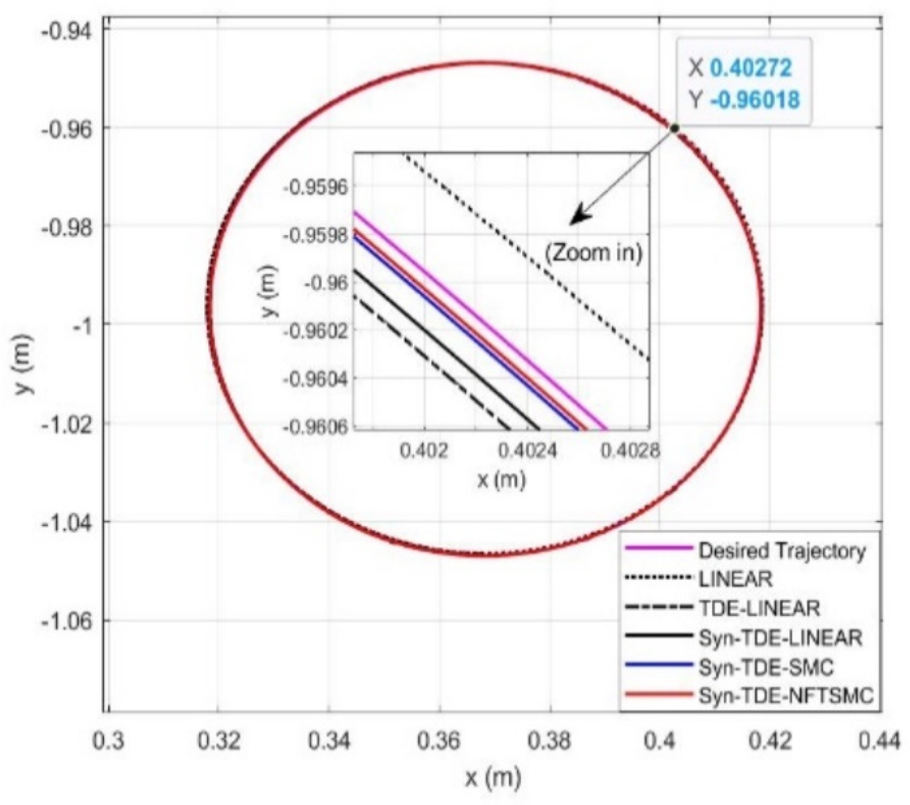
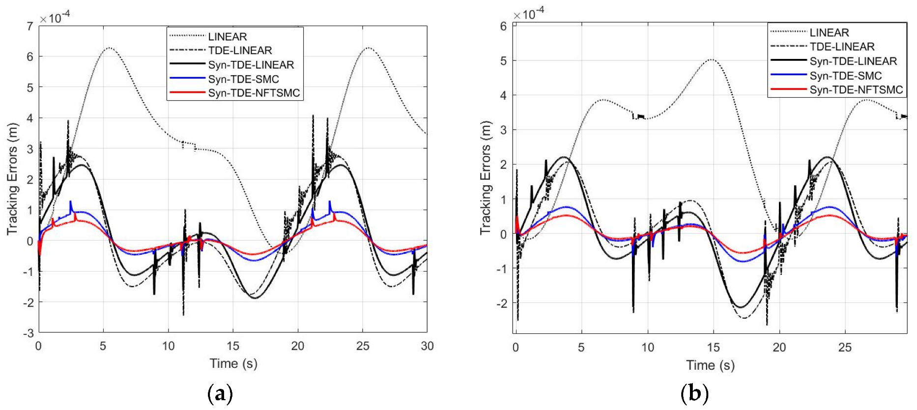
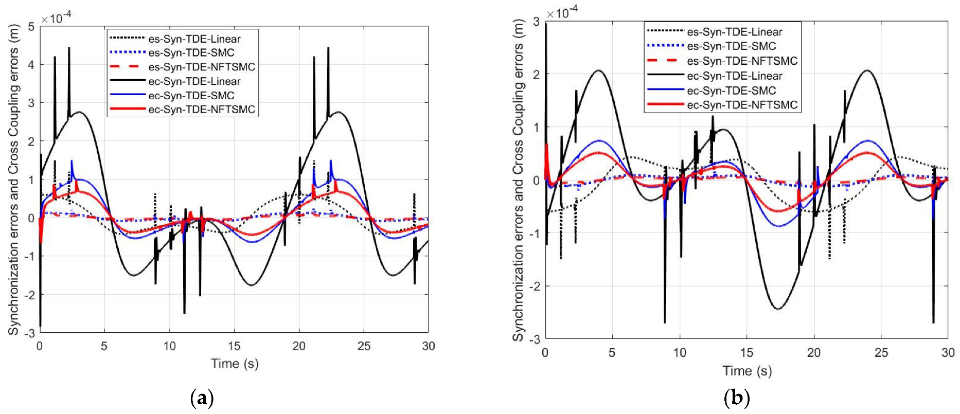
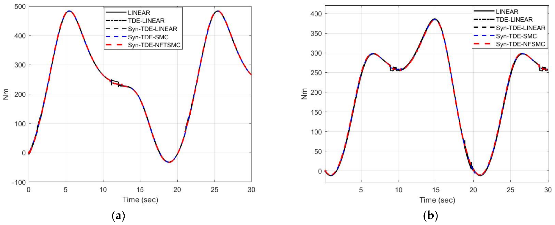
6.2. Simulation Results

The control schemes listed in Table 2 are used in the computer simulation to control the end-effector of the manipulator to track a circle specified by x d e s ( t ) and y d e s ( t ) as follows.
{ x d e s ( t ) = 0.3683 + 0.05 cos ( π t + π / 2 ) y d e s ( t ) = 0.4183 0.05 sin ( π t / 10 + π / 2 )
The results obtained from the simulation are presented in Figure 5, Figure 6, Figure 7, Figure 8 and Figure 9 and Table 3, Table 4 and Table 5. Figure 5 shows the planar motions of the manipulator end-effector when controlled by the above control schemes while Figure 6 presents the time trajectories of the tracking errors e ( t ) of the control schemes. Table 3 tabulates the absolute average tracking errors (AATE) of the control schemes computed by MATLAB.
Figure 7 presents the time trajectories of the synchronization errors ( e s ( t ) ) and cross-coupling ( e c ( t ) ) of the control schemes while Figure 8 presents the estimation errors ( e e s t ( t ) ) of the Syn-TDE-NFTSMC. Table 4 tabulates the absolute average synchronization errors (AASE) and cross-coupling errors (AACE) of the control schemes while Table 5 tabulates the absolute average estimation errors (AAEE) of the Syn-TDE-NFTSMC, computed by MATLAB.
The control inputs of both joints show no chattering, as shown in Figure 9a,b.
From Figure 5, Figure 6 and Figure 7, it is seen that Syn-TDE-LINEAR provided better performance and faster error convergence than both LINEAR and TDE-LINEAR. It is meaningful that the involvement of TDE and the synchronization errors improved the performance of the control schemes. Syn-TDE-SMC showed a better tracking path than the Syn-TDE-LINEAR. Finally, we see that our proposed control scheme, Syn-TDE-NFTSMC, was on track with the fastest desired trajectory with the slightest deviation (from the desired path in Figure 5) and had the fastest error convergence compared to other existing control schemes.
From Table 3, based on the computed AATEs of the control scheme, it is clear that inclusion of TDE and the synchronization errors improved the performance of control schemes as for example the AATE of the TDE-LINEAR (0.0197 mm) is smaller than that of the LINEAR (0.32 mm). Other AATEs in the table validate the above observation. From the results presented in Table 3, we see that our proposed control scheme, namely Syn-TDE-NFTSMC, has the best tracking performance as compared to other existing control schemes due to its smallest AATEs for both joint variables.
From Table 4, based on the computed AASEs and AACEs of the control scheme, it is clear that inclusion of Syn-TDE-NFTSMC improved the performance of control schemes as for example the AASEs of the Syn-TDE-NFTSMC ( 2.16 × 10 3 mm) is smaller than that of the Syn-TDE-SMC ( 3.82 × 10 3 mm). Other AASEs and AACEs in the table validate the above observation. From the results presented in Table 4, we see that our proposed control scheme has the best tracking performance as compared to other existing control schemes due to its smallest AASEs and AACEs for both joint variables.
Figure 8a,b plotted the nonlinear term H i = H ( q , q ˙ , q ¨ ) , the estimation term h i = τ t L M ¯ q ¨ t L , and the estimation error e e s t i = H i h i = H ( q , q ˙ , q ¨ ) ( τ t L M ¯ q ¨ t L ) , respectively, of the ith active joint. It can be seen that the estimation error remains close to zero. Furthermore, from the results presented in Table 5, we see that our proposed control scheme, namely Syn-TDE-NFTSMC, has the AAEEs close to zero as 0.0177 Nm and 0.0172 Nm for both joint variables. This implies that the TDE cancels the uncertainty, and the chattering phenomenon is reduced while maintaining the tracking accuracy.
Therefore, it can be concluded that the proposed control scheme shows high-accuracy tracking performance with the model-free control performance in comparison with the other control schemes.

7. Conclusions

In this paper, we proposed a new NFTSMC scheme in which TDE was applied to efficiently compute the dynamics of a robot manipulator and disturbances required for control scheme. In addition, the synchronization errors were used instead of the conventional joint errors. A new NFTSMC law was proposed and the Lyapunov Theorem was employed to prove that the proposed control scheme is uniformly stable. The conducted computer simulation showed that the proposed control scheme provided the best tracking performance compared with other existing control schemes including LINEAR, TDE-based LINEAR, TDE-based LINEAR with synchronization errors, and TDE-based SMC with synchronization errors when tracking the same motion for a 2-DOF-CKCM.
Comparing with the existing approach, the proposed control scheme has several significant improvements:
(1)
The proposed control scheme optimally synchronized the robot joints to minimize the synchronization errors with an NFTSMC-based controller.
(2)
Since the proposed control scheme does not require the computation of the manipulator dynamics thanks to TDE, it is computationally efficent and is, therefore, suitable for real-time control applications.
Future work from this paper could include computer simulation study on higher DOF manipulators and experimental studies of the proposed control scheme on real manipulators.

Author Contributions

Conceptualization, T.T.C.D., C.C.N. and T.D.T.; methodology, T.T.C.D. and C.C.N.; software, T.T.C.D. and C.C.N.; validation, T.T.C.D. and C.C.N.; results analysis, T.T.C.D. and T.D.T.; investigation, C.C.N., T.T.C.D. and T.D.T.; data curation, T.T.C.D. and T.D.T.; writing—original draft preparation, C.C.N., T.T.C.D. and T.D.T.; writing—review and editing, C.C.N. and T.T.C.D.; visualization, C.C.N. and T.T.C.D.; supervision, C.C.N. and T.T.C.D. All authors have read and agreed to the published version of the manuscript.

Funding

This research received no external funding.

Institutional Review Board Statement

Not applicable.

Informed Consent Statement

Not applicable.

Data Availability Statement

Not applicable.

Conflicts of Interest

All authors announce that they have no conflict of interest in relation to the publication of this article.

Appendix A. Other Control Schemes Used in Computer Simulation

This appendix contains relevant equations of control schemes to which the proposed control scheme is compared to in our computer simulation study.
LINEAR
The LINEAR and TDE-LINEAR Control Scheme were suggested in Reference [22] given by the following.
τ = M ¯ ( q ¨ d + K D e ˙ + K P e )
where K D and K P are constant matrices.
TDE-based LINEAR (TDE-LINEAR)
τ = τ t L M ¯ q ¨ t L TDE + M ¯ ( q ¨ d + K D e ˙ + K P e ) LINEAR   control
TDE-based LINEAR with synchronization errors (Syn-TDE-LINEAR)
τ = τ t L M ¯ q ¨ t L TDE + M ¯ ( q ¨ d + K D e ˙ c + K P e c ) LINEAR   control
TDE-based SMC with synchronization errors (Syn-TDE-SMC)
The control scheme was suggested in Reference [13] and is given by the following:
τ = τ t L M ¯ q ¨ t L TDE + M ¯ ( q ¨ d + K e ˙ c + K s w sign ( s ) + K 1 s ) SMC   control
where the sliding surface expressed by s = e ˙ c + K e c .

References

  1. Patel, Y.D.; George, P.M. Parallel Manipulators Applications—A Survey. Mod. Mech. Eng. 2012, 2, 57–64. [Google Scholar] [CrossRef] [Green Version]
  2. Nguyen, C.C.; Pooran, F.J. Kinematic analysis and workspace determination of a 6 dof CKCM robot end-effector. J. Mech. Work. Technol. 1989, 20, 283. [Google Scholar] [CrossRef]
  3. Nguyen, C.C.; Pooran, F.J. Dynamic analysis of a 6 DOF CKCM robot end-effector for dual-arm telerobot systems. Robot. Auton. Syst. 1989, 5, 377. [Google Scholar] [CrossRef]
  4. Nguyen, C.C.; Sam, S.A.; Zhen, L.Z.; Campbell, C.E., Jr. Adaptive control of a stewart platform-based manipulator. J. Robot. Syst. 1993, 10, 657. [Google Scholar] [CrossRef]
  5. Koren, Y. Cross-Coupled Biaxial Computer Control for Manufacturing Systems. J. Dyn. Syst. Meas. Control 1980, 102, 265. [Google Scholar] [CrossRef]
  6. Doan, Q.V.; Le, T.D.; Vo, A.T. Synchronization Full-Order Terminal Sliding Mode Control for an Uncertain 3-DOF Planar Parallel Robotic Manipulator. Appl. Sci. 2019, 9, 1756. [Google Scholar] [CrossRef] [Green Version]
  7. Zhao, D.; Li, S.; Gao, F. Finite time position synchronised control for parallel manipulators using fast terminal sliding mode. Int. J. Syst. Sci. 2009, 40, 829. [Google Scholar] [CrossRef]
  8. Nguyen, T.T. Intelligent Control of Closed-Kinematic Chain Robot Manipulators. Ph.D. Thesis, The Catholic University of America, Washington, DC, USA, 2020. [Google Scholar]
  9. Su, Y.; Sun, D.; Ren, L.; Mills, J.K. Integration of saturated PI synchronous control and PD feedback for control of parallel manipulators. IEEE Trans. Robot. A Publ. IEEE Robot. Autom. Soc. 2006, 22, 202. [Google Scholar] [CrossRef]
  10. Sang, C.; Cong, S. Nonlinear computed torque control for a high-speed planar parallel manipulator. Mechatronics 2009, 19, 987. [Google Scholar] [CrossRef]
  11. Chung, S.J.; Slotine, J.J.E. Cooperative robot control and synchronization of Lagrangian systems. In Proceedings of the 46th IEEE Conference on Decision and Control, New Orleans, LA, USA, 12–14 December 2007. [Google Scholar]
  12. Nuno, E.; Basanez, L.; Ortega., R. Adaptive control for the synchronization of multiple robot manipulators with coupling time-delays. In Proceedings of the IEEE/RSJ International Conference on Intelligent Robots and Systems, Taipei, Taiwan, 18–22 October 2010. [Google Scholar] [CrossRef]
  13. Duong, T.; Tran, T.D.; Nguyen, T.T.; Duong, V.N. Synchronization Sliding Mode Control with Time-Delay Estimation for a 2-DOF Closed-Kinematic Chain Robot Manipulator. In Proceedings of the International Conference on System Science and Engineering (ICSSE), Ho Chi Minh City, Vietnam, 26–28 August 2021. [Google Scholar] [CrossRef]
  14. Bouaziz, F.A.; Bouteraa, Y.; Medhaffar, H. Distributed sliding mode control of cooperative robotic manipulators. In Proceedings of the 10th International Multi-Conferences on Systems, Signals & Devices 2013 (SSD13), Hammamet, Tunisia, 18–21 March 2013. [Google Scholar] [CrossRef]
  15. Zhao, D.; Li, S.; Gao, F. Fully adaptive feedforward feedback synchronized tracking control for Stewart Platform systems. Int. J. Control Autom. Syst. 2008, 6, 689–701. [Google Scholar]
  16. Su, Y.X.; Sun, D.; Ren, L.; Wang, X.; Mills, J.K. Nonlinear PD Synchronized Control for Parallel Manipulators. In Proceedings of the 2005 IEEE International Conference on Robotics and Automation, Barcelona, Spain, 18–22 April 2005. [Google Scholar] [CrossRef]
  17. Zhao, D.; Li, S.; Gao, F. A new terminal sliding mode control for robotic manipulators. Int. J. Control 2009, 82, 1804. [Google Scholar] [CrossRef]
  18. Zhihong, M.; Paplinski, A.P.; Wu, H.R. A robust MIMO terminal sliding mode control scheme for rigid robotic manipulators. IEEE Trans. Autom. Control 1994, 39, 2464. [Google Scholar] [CrossRef]
  19. Tang, Y. Terminal sliding mode control for rigid robots. Automatica 1998, 34, 51. [Google Scholar] [CrossRef]
  20. Yang, L.; Yang, J. Nonsingular fast terminal sliding-mode control for nonlinear dynamical systems. Int. J. Robust Nonlinear Control 2011, 21, 1865. [Google Scholar] [CrossRef]
  21. Van, M.; Ge, S.S.; Ren, H. Finite Time Fault Tolerant Control for Robot Manipulators Using Time Delay Estimation and Continuous Nonsingular Fast Terminal Sliding Mode Control. IEEE Trans. Cybern. 2017, 47, 1681. [Google Scholar] [CrossRef]
  22. Hsia, T.C.S.; Lasky, T.A.; Guo, Z. Robust independent joint controller design for industrial robot manipulators. IEEE Trans. Ind. Electron. A Publ. IEEE Ind. Electron. Soc. 1991, 38, 21. [Google Scholar] [CrossRef]
  23. Baek, J.; Cho, S.; Han, S. Practical Time-Delay Control with Adaptive Gains for Trajectory Tracking of Robot Manipulators. IEEE Trans. Ind. Electron. A Publ. IEEE Ind. Electron. Soc. 2018, 65, 5682. [Google Scholar] [CrossRef]
  24. Bae, H.-J.; Jin, M.; Suh, J.; Lee, J.Y.; Chang, P.-H.; Ahn, D.-s. Control of Robot Manipulators Using Time-Delay Estimation and Fuzzy Logic Systems. J. Electr. Eng. Technol. 2017, 12, 1271. [Google Scholar] [CrossRef] [Green Version]
  25. Maolin, J.; Jinoh, L.; Pyung, H.C.; Chintae, C. Practical Nonsingular Terminal Sliding-Mode Control of Robot Manipulators for High-Accuracy Tracking Control. IEEE Trans. Ind. Electron. A Publ. IEEE Ind. Electron. Soc. 2009, 56, 3593. [Google Scholar] [CrossRef]
  26. Kelly, R.; Davila, V.S.; Loría, A. Control of Robot Manipulators in Joint Space, 1st ed.; Springer: London, UK, 2005; pp. XXVI, 426. [Google Scholar] [CrossRef]
  27. Xu, Z.; Huang, W.; Li, Z.; Hu, L.; Lu, P. Nonlinear Nonsingular Fast Terminal Sliding Mode Control Using Deep Deterministic Policy Gradient. Appl. Sci. 2021, 11, 4685. [Google Scholar] [CrossRef]
  28. Feng, Y.; Yu, X.; Man, Z. Non-singular terminal sliding mode control of rigid manipulators. Automatica 2002, 38, 2159. [Google Scholar] [CrossRef]
  29. Shtessel, Y.; Edwards, C.; Fridman, L.; Levant, A. Sliding Mode Control and Observation; Birkhäuser: Basel, Switzerland, 2014. [Google Scholar]
  30. Su, W.-C.; Drakunov, S.V.; Ozguner, U. An O(T/sup 2/) boundary layer in sliding mode for sampled-data systems. IEEE Trans. Autom. Control 2000, 45, 482. [Google Scholar] [CrossRef]
  31. Spong, M.; Vidyasagar, M. Robust linear compensator design for nonlinear robotic control. IEEE Trans. Robot. Autom. A Publ. IEEE Robot. Autom. Soc. 1987, 3, 345. [Google Scholar] [CrossRef]
  32. Brunton, S.L.; Kutz, J.N. Data-Driven Science and Engineering; Cambridge University Press: Cambridge, UK, 2019. [Google Scholar] [CrossRef] [Green Version]
  33. Pooran, J.F. Dynamics and Control of Robot Manipulators with Closed-Kinematic Chain Mechanism. Ph.D. Thesis, The Catholic University of America, Washington, DC, USA, 1989. [Google Scholar]
Figure 1. Architecture of the 2 DOF CKCM manipulator.
Applsci 12 05527 g001
Figure 2. Frame assignment for the 2 DOF planar CKCM manipulator.
Applsci 12 05527 g002
Figure 3. Structure of the Proposed Control Scheme.
Applsci 12 05527 g003
Figure 4. Control design in MatLab/Simulink environment.
Applsci 12 05527 g004
Figure 5. Trajectory tracking in X-Y plane (circular motion).
Applsci 12 05527 g005
Figure 6. Time trajectories of tracking errors of the control schemes, of joint 1 (a) and joint 2 (b).
Applsci 12 05527 g006
Figure 7. Time trajectories of synchronization errors and cross coupling errors of the control schemes, of joint 1 (a) and joint 2 (b).
Applsci 12 05527 g007
Figure 8. Time trajectories of estimation errors of Syn-TDE-NFTSMC of joint 1 (a) and joint 2 (b).
Applsci 12 05527 g008
Figure 9. The control input signals of the control schemes of joint 1 (a) and joint 2 (b).
Applsci 12 05527 g009
Table 1. The robot parameters.
Robot ParametersDescriptionValueUnit
m Link’s total mass4.91kg
m 1 Link’s moving part mass0.59kg
d Grounds’ horizontal distance0.74m
l s Link’s fixed length0.26m
F V 1 Viscous friction coefficient of the 1st link5N·m·s/rad
F V 2 Viscous friction coefficient of the 2nd link5N·m·s/rad
F C 1 Coulomb friction coefficient of the 1st link5N·m
F C 2 Coulomb friction coefficient of the 2nd link5N·m
gGravitational acceleration constant9.81m/s2
Table 2. The parameters of the control schemes.
Control SchemeControl Parameters
LINEAR M ¯ = diag ( 0.1 ,   0.1 ) ,   K D = diag ( 200 ,   200 ) ,   K P = diag ( 7.704 × 10 3 , 7.704 × 10 3 )
TDE-LINEAR L = 9.999 × 10 4 s ,   M ¯ = diag ( 0.1 ,   0.1 ) ,   K D = diag ( 200 ,   200 ) ,   K P = diag ( 7.704 × 10 3 , 7.704 × 10 3 )
Syn-TDE-LINEAR L = 9.999 × 10 4 s ,   M ¯ = diag ( 0.1 ,   0.1 ) ,   K D = diag ( 200 ,   200 ) ,   K P = diag ( 7.704 × 10 3 , 7.704 × 10 3 ) ,   α = diag(0.5,0.5)
Syn-TDE-SMC L = 9.999 × 10 4 s ,   M ¯ = diag ( 0.1 ,   0.1 ) ,   K 1 = diag ( 0.1 ,   0.1 ) ,   K = diag ( 10 ,   10 ) ,   K s w = diag ( 5 ,   5 ) ,   α = diag(0.5, 0.5)
Syn-TDE-NFTSMC L = 9.999 × 10 4 s ,   p 1 = 19 ,   p 2 = 11 ,   q 1 = 17 ,   q 2 = 9 ,   M ¯ = diag ( 0.1 ,   0.1 ) ,   K 1 = diag ( 25 ,   25 ) ,   K 2 = diag ( 5 ,   5 ) ,   K = diag ( 0.1 ,   0.1 ) ,   K s w = diag ( 15 ,   15 ) ,   α = diag ( 0.5 ,   0.5 )
Table 3. The absolute average tracking errors (AATE) of the control schemes, computed by MATLAB.
Tracking ErrorsLINEARTDE-LINEARSyn-TDE-LINEARSyn-TDE-SMCSyn-TDE-NFTSMC
e 1 (mm)0.320.01970.0197 7.17 × 10 3 4.07 × 10 3
e 2 (mm)0.260.01920.0192 6.95 × 10 3 5.06 × 10 3
Table 4. The absolute average synchronization errors (AASE) and cross-coupling errors (AACE) of the control schemes, computed by MATLAB.
Tracking ErrorsSyn-TDE-LINEARSyn-TDE-SMCSyn-TDE-NFTSMC
e s 1 (mm)0.0206 3.82 × 10 3 2.16 × 10 3
e s 2 (mm)0.0206 3.82 × 10 3 2.16 × 10 3
e c 1 (mm)0.028 1.03 × 10 2 9.07 × 10 3
e c 2 (mm)0.016 5.33 × 10 3 4.99 × 10 3
Table 5. The absolute average estimation errors (AAEE) of the Syn-TDE-NFTSMC computed by MATLAB.
AAEESyn-TDE-NFTSMC
e e s t 1 (Nm)0.0177
e e s t 2 (Nm)0.0172
Publisher’s Note: MDPI stays neutral with regard to jurisdictional claims in published maps and institutional affiliations.

