
A Double-Level Calculation Model for the Construction Schedule Planning of Urban Rail Transit Network


Abstract
1. Introduction
2. Model Formulation
2.1. Rough Set and Improved TOPSIS Construction Sequence Sub-Model
- (1)
- The weightings used in the TOPSIS method are determined using qualitative methods, such as expert scoring (ES), and weighted arithmetic average (WAA). This will affect the accuracy of the ranking results. Since Rough Set theory was first proposed by Pawlak in 1982 [35,36], it has been used to improve the weight problem in many studies [37,38,39]. In this study, the Rough Set classification mechanism was used to intelligently calculate the attribute weight to solve the problem of the subjectivity of attribute weighting in TOPSIS.
- (2)
- The TOPSIS method just sets up two ideal solutions, namely the positive ideal solution (PIS) and the negative ideal solution (NIS). Its core idea is to find an optimal solution close to the positive ideal solution and far away from the negative ideal solution. However, when the distances between the alternatives and the ideal solution are equal, the TOPSIS method cannot rank the alternatives. In this study, an ideal solution set is designed to solve this limitation of TOPSIS.
2.2. Logistic-β Construction Timing Sub-Model
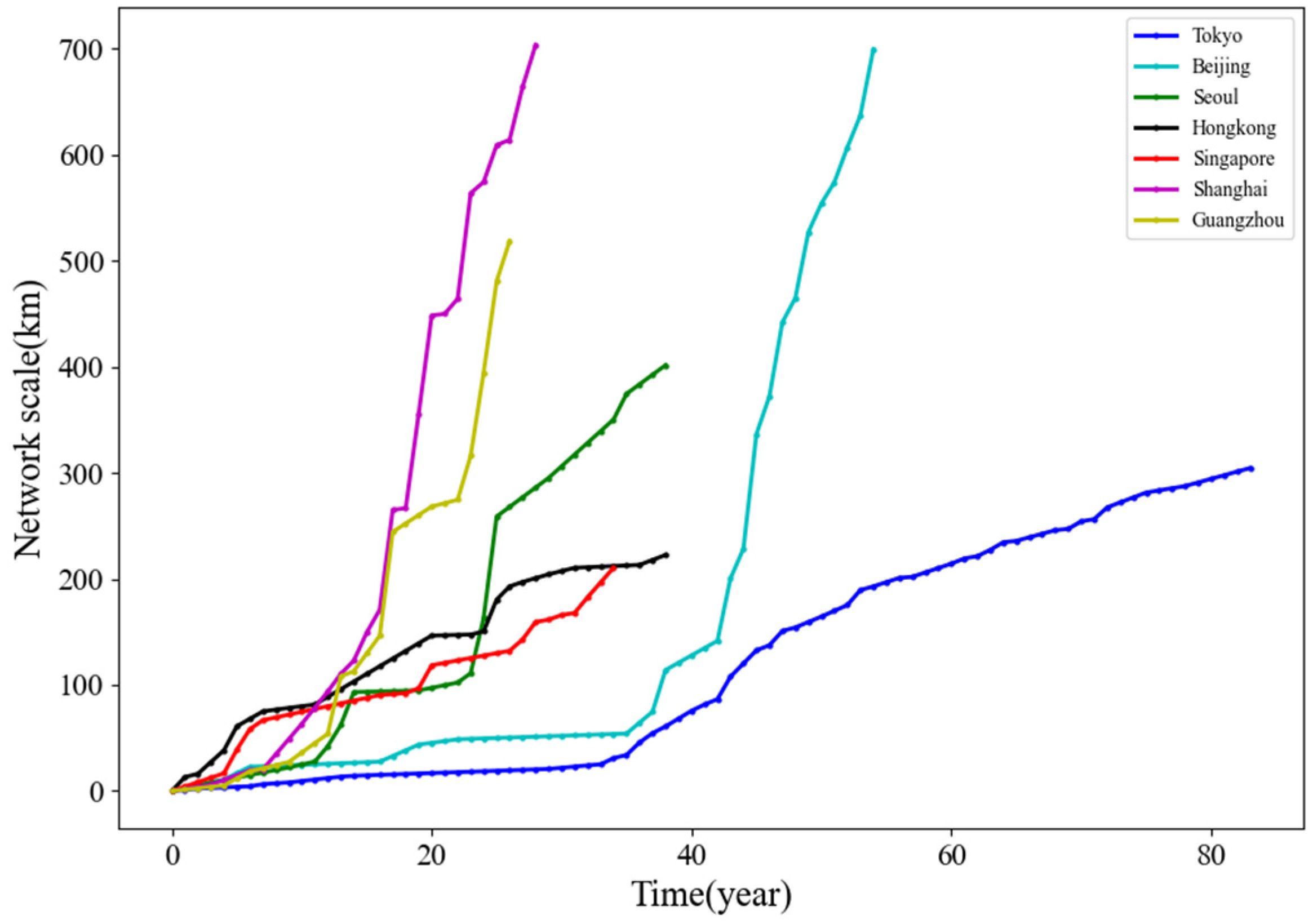
2.2.1. The URT Network Growth Curve
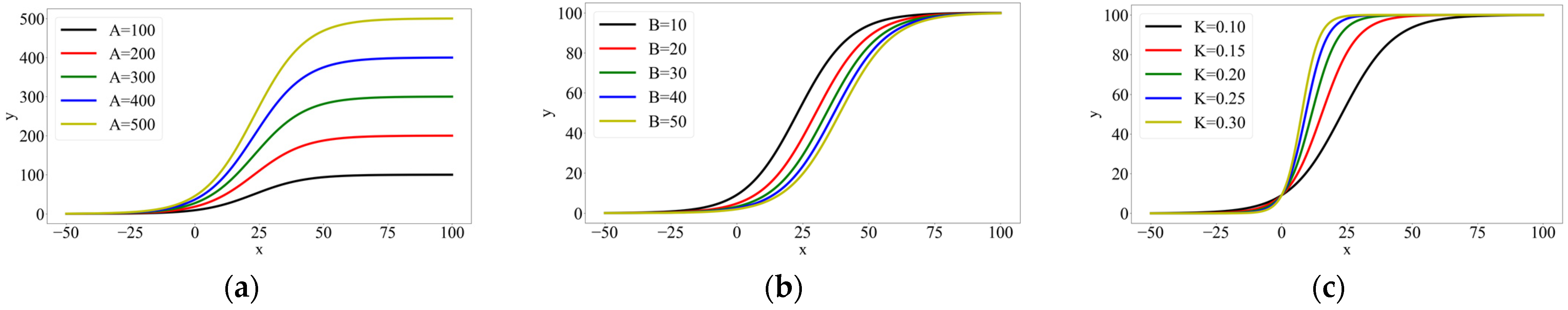
2.2.2. Parameter Analysis
2.2.3. Construction Timing
3. Case Study
3.1. Input Data and Results
3.1.1. Input and calculate Data
3.1.2. Output Results
3.2. Discussion
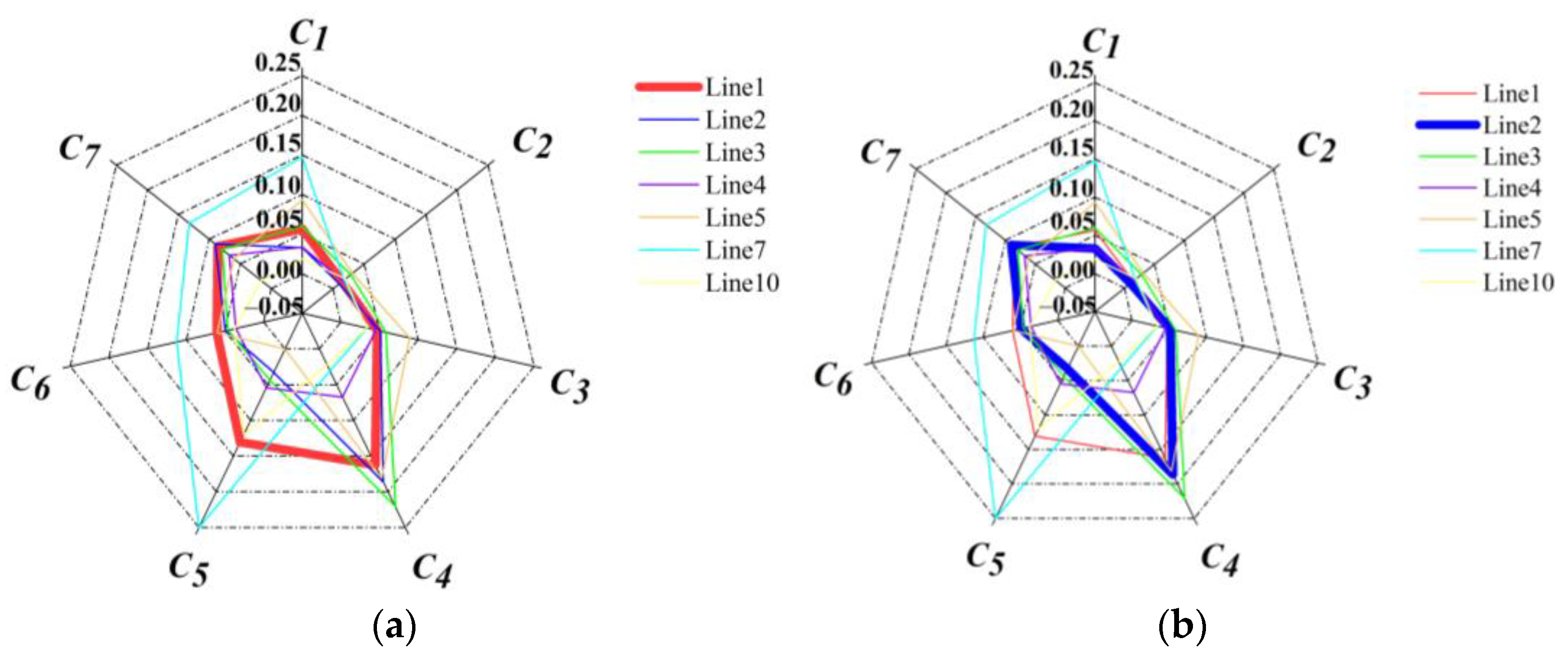
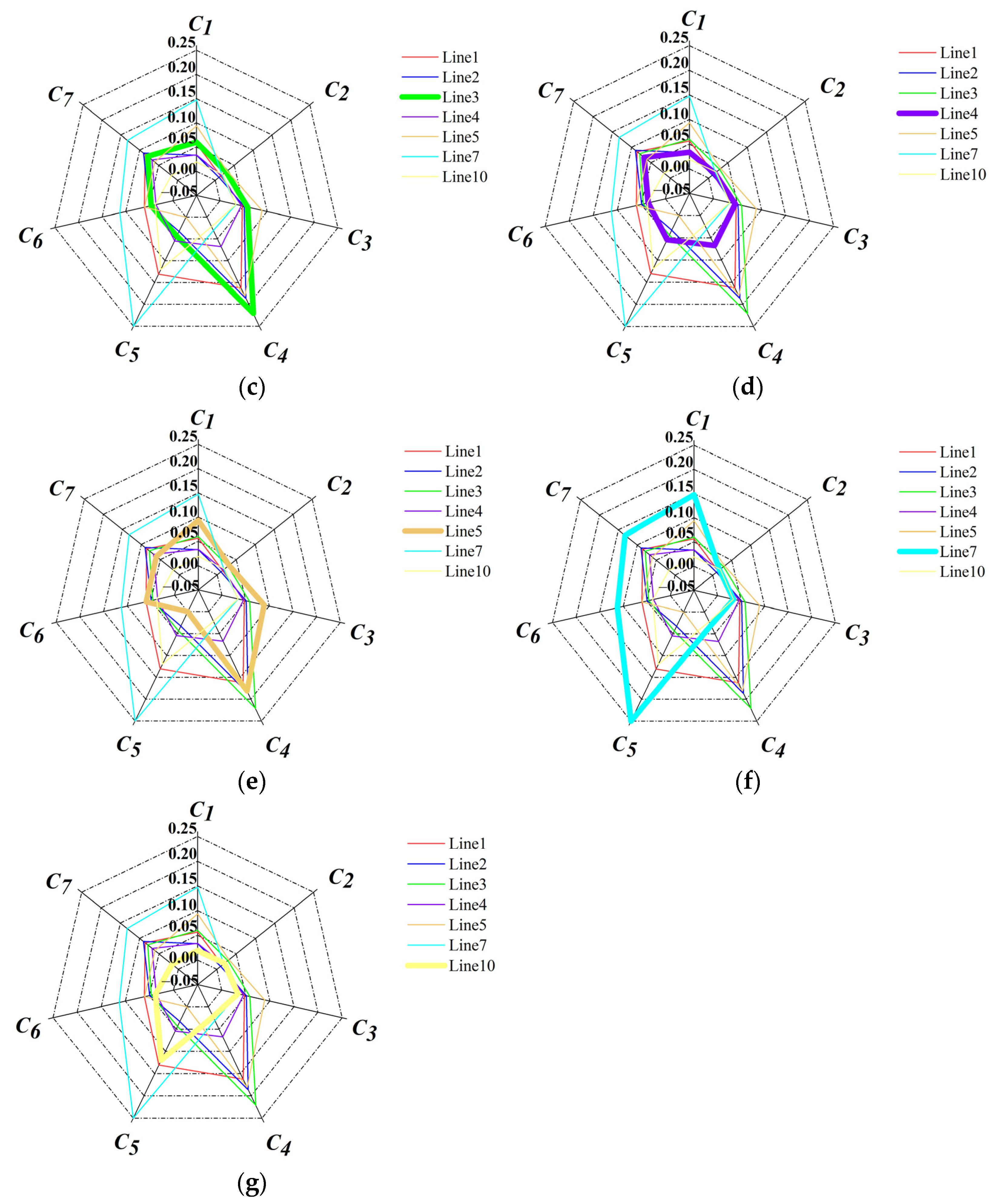
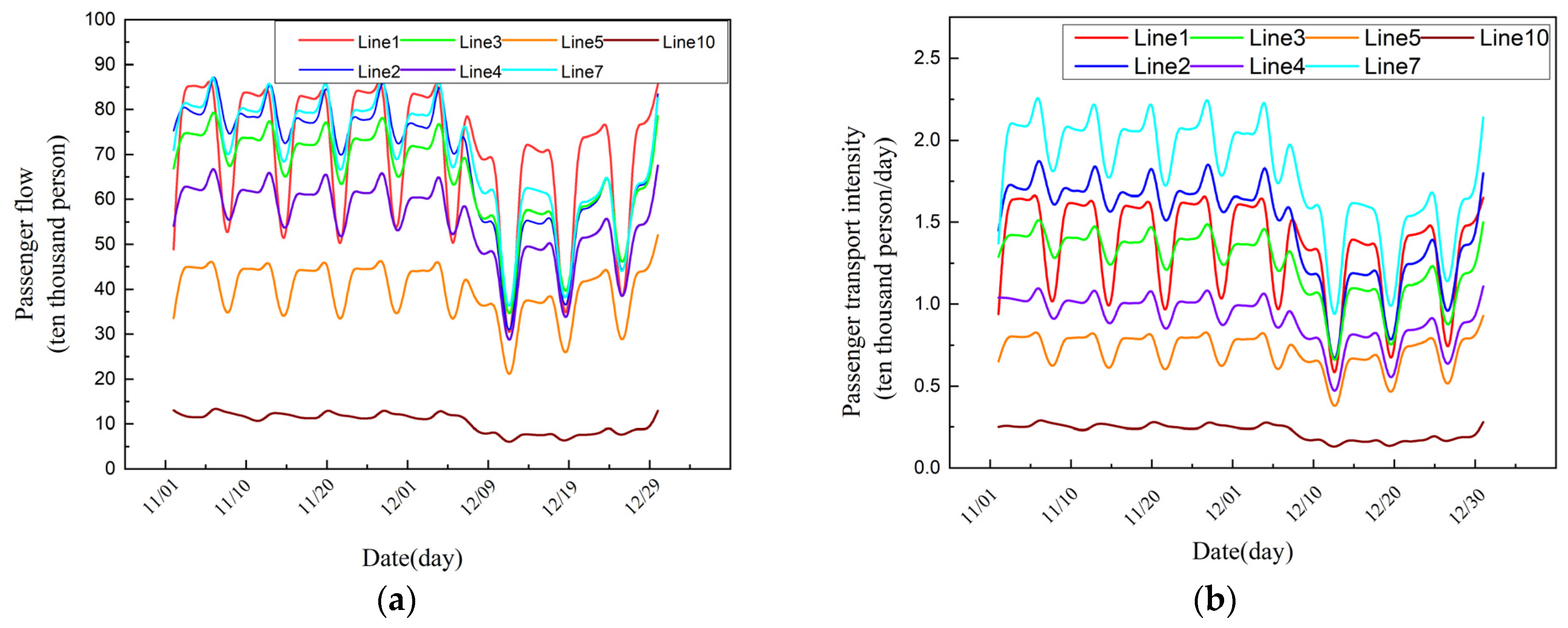
3.2.1. Analysis of the Construction Sequence
- (1)
- Decision indicators
- (2)
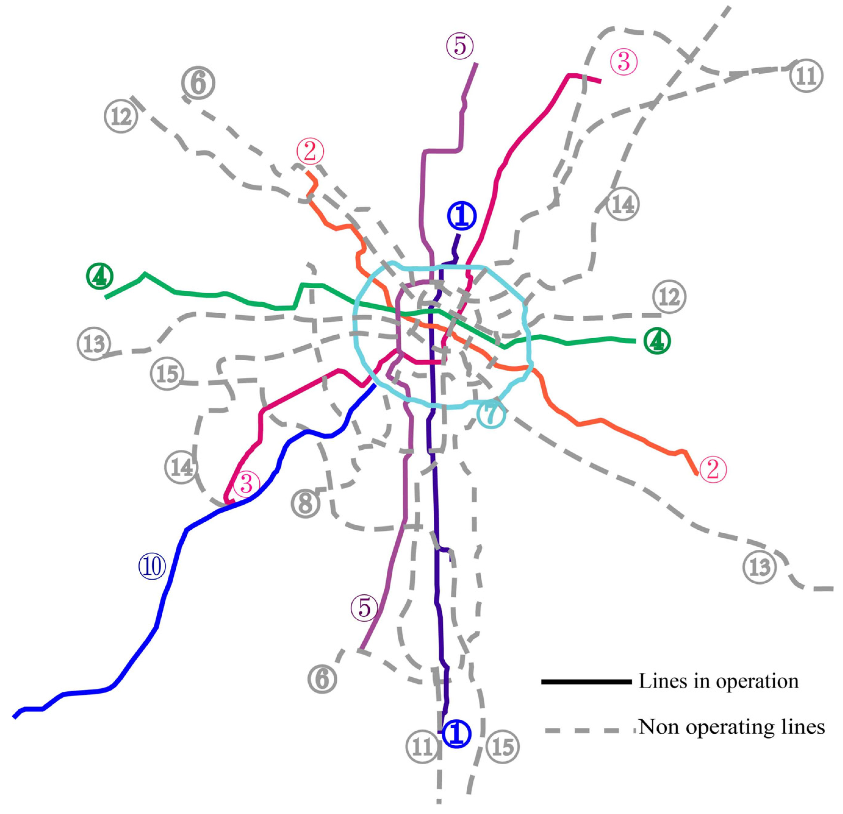
- The construction sequence
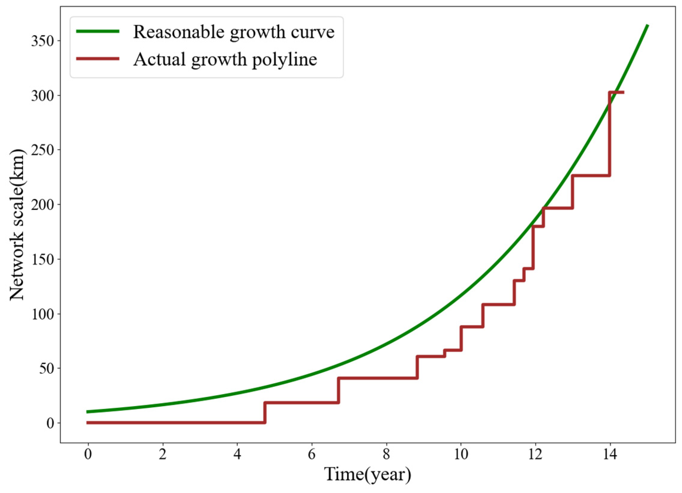
3.2.2. Analysis of Construction Timing
- (1)
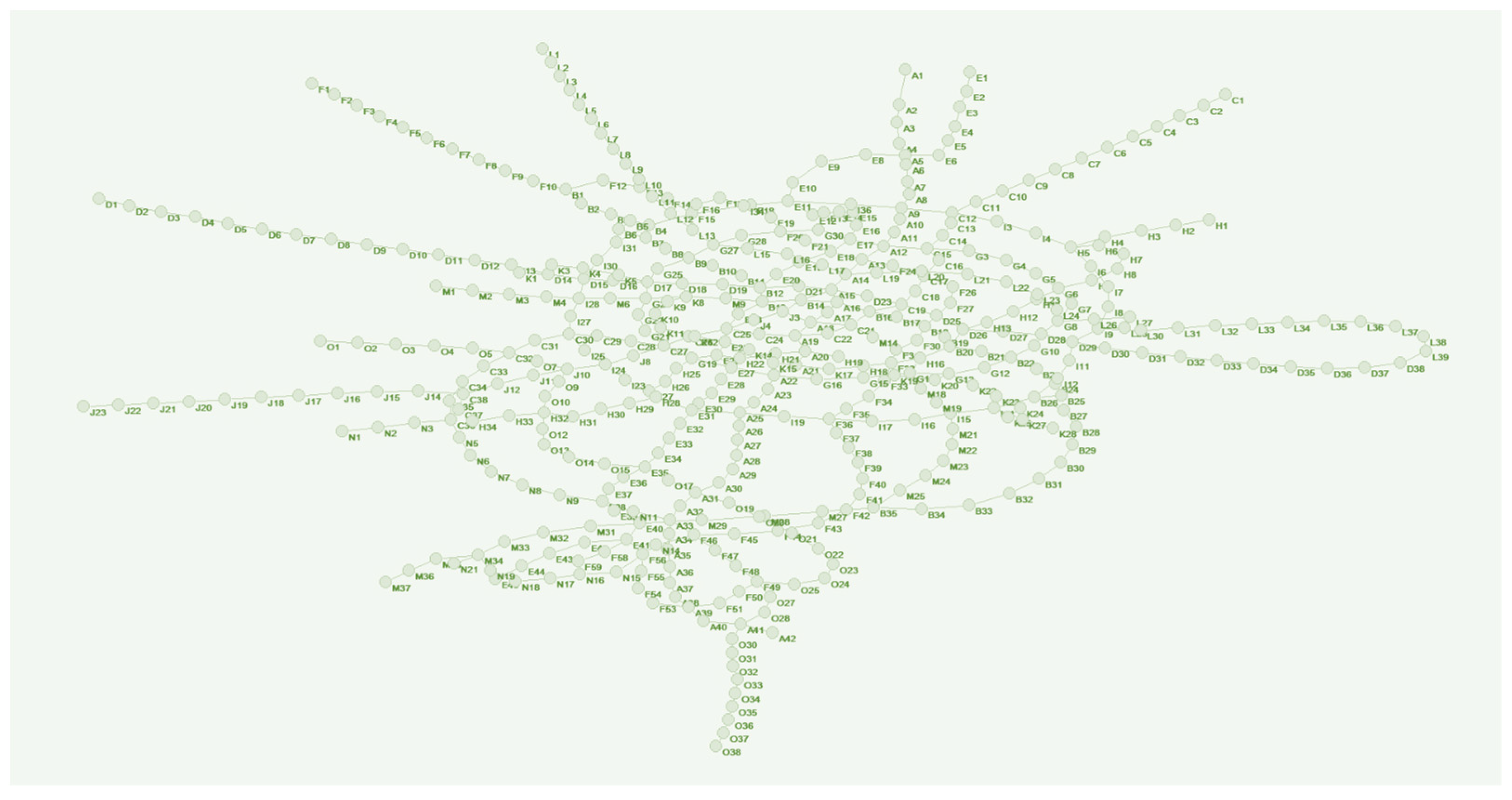
- The growth curve of Chengdu rail transit network
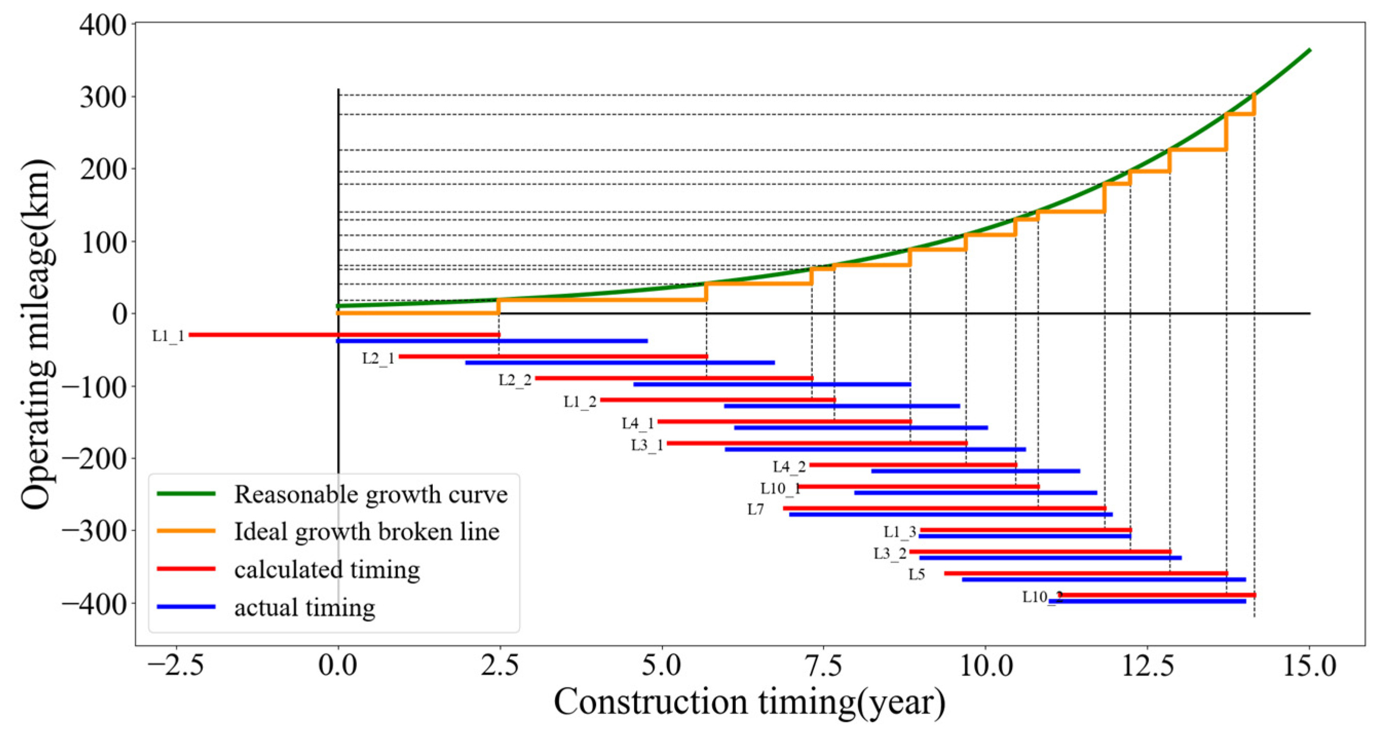
- (2)
- The discussion of construction timing
4. Conclusions
Author Contributions
Funding
Institutional Review Board Statement
Informed Consent Statement
Data Availability Statement
Conflicts of Interest
Appendix A

| Lines | Line Length (km) | Daily Passenger Volume (Ten Thousand People) | Average Transportation Distance (km) | Peak Section Flow (Ten Thousand People/h) |
|---|---|---|---|---|
| Line 1 | 51.88 | 141.42 | 6.81 | 3.58 |
| Line 2 | 46.42 | 98.63 | 7.94 | 3.74 |
| Line 3 | 52.49 | 145.08 | 10.79 | 3.77 |
| Line 4 | 60.89 | 110.47 | 8.09 | 3.60 |
| Line 5 | 55.85 | 198.51 | 8.10 | 4.54 |
| Line 6 | 73.51 | 242.58 | 9.21 | 4.13 |
| Line 7 | 38.62 | 183.43 | 6.26 | 3.08 |
| Line 8 | 44.05 | 115.30 | 10.40 | 3.38 |
| Line 9 | 68.92 | 158.68 | 10.75 | 3.71 |
| Line 10 | 46.25 | 81.92 | 12.36 | 2.79 |
| Line 11 | 30.05 | 41.92 | 7.74 | 2.26 |
| Line 12 | 58.31 | 76.94 | 9.24 | 2.01 |
| Line 13 | 91.69 | 124.73 | 12.18 | 3.27 |
| Line 14 | 75.13 | 94.05 | 12.89 | 3.16 |
| Line 15 | 54.07 | 109.07 | 5.68 | 2.63 |
| Lines | Line Length (km) | Daily Passenger Volume (Ten Thousand People) | Average Transportation Distance (km) | Peak Section Flow (Ten Thousand People/h) |
|---|---|---|---|---|
| Line 1 | 51.88 | 144.20 | 6.33 | 3.80 |
| Line 2 | 46.42 | 102.92 | 7.05 | 3.86 |
| Line 3 | 52.49 | 153.22 | 9.94 | 4.26 |
| Line 4 | 60.89 | 155.82 | 7.30 | 3.66 |
| Line 5 | 55.85 | 209.66 | 8.25 | 5.27 |
| Line 6 | 73.51 | 253.78 | 9.03 | 5.30 |
| Line 7 | 38.62 | 200.26 | 5.09 | 3.51 |
| Line 8 | 44.05 | 124.39 | 9.72 | 3.92 |
| Line 9 | 68.92 | 175.64 | 8.82 | 4.67 |
| Line 10 | 46.25 | 87.17 | 15.08 | 3.78 |
| Line 11 | 30.05 | 43.89 | 7.47 | 2.89 |
| Line 12 | 58.31 | 83.08 | 9.05 | 2.59 |
| Line 13 | 91.69 | 148.90 | 12.54 | 4.18 |
| Line 14 | 75.13 | 116.86 | 12.42 | 3.98 |
| Line 15 | 54.07 | 116.31 | 7.56 | 3.15 |
References
- Song, P.; Yang, Q.F. Empirical Research on Construction Scheduling for Urban Rail Transit Network. In Proceedings of the 4th International Conference on Wireless Communications, Networking and Mobile Computing, Dalian, China, 12–14 October 2008; pp. 1–5. [Google Scholar] [CrossRef]
- Cipriani, E.; Gori, S.; Petrelli, M. Transit network design: A procedure and an application to a large urban area. Transp. Res. Part C-Emer. 2010, 20, 3–14. [Google Scholar] [CrossRef]
- Laporte, G.; Mesa, J.A. The Design of Rapid Transit Networks. In Location Science; Springer: Cham, Switzerland, 2015; pp. 581–594. [Google Scholar] [CrossRef]
- Cadarso, L.; Marín, Á. Improved rapid transit network design model: Considering transfer effects. Ann. Oper. Res. 2017, 258, 547–567. [Google Scholar] [CrossRef]
- Chai, S.; Liang, Q.; Zhong, S. Design of Urban Rail Transit Network Constrained by Urban Road Network, Trips and Land-Use Characteristics. Sustainability 2019, 11, 6128. [Google Scholar] [CrossRef]
- Liu, B.; Zhu, G.Y.; Li, X.L.; Sun, R.R. Vulnerability Assessment of the Urban Rail Transit Network Based on Travel Behavior Analysis. IEEE Access 2021, 9, 1407–1419. [Google Scholar] [CrossRef]
- Yang, T.Y.; Zhao, P.; Qiao, K.; Yao, X.M.; Wang, T. Vulnerability Analysis of Urban Rail Transit Network by Considering the Station Track Layout and Passenger Behavior. J. Adv. Transp. 2021, 2021, 6378526. [Google Scholar] [CrossRef]
- Zhang, Y.X.; Zhou, X.; Luo, J.; Zhang, Z.L. Urban Traffic Dynamics Prediction—A Continuous Spatial-temporal Meta-learning Approach. ACM Trans. Intell. Syst. Technol. 2022, 13, 1–19. [Google Scholar] [CrossRef]
- Luo, X.Q.; Guo, Y.Y.; Wu, Y. The Timing of Urban Rail Transit Construction Based on the Weighted Gray Correlation. App. Mech. Mater. 2011, 97–98, 1189–1194. [Google Scholar] [CrossRef]
- Peng, W.T.; Li, Z.C.; Schonfeld, P. Development of Rail Transit Network over Multiple Time Periods. Transp. Res. Part A-Policy Pract. 2019, 121, 235–250. [Google Scholar] [CrossRef]
- Cheng, W.C.; Schonfeld, P.A. Method for Optimizing the Phased Development of Rail Transit Lines. Urban Rail Transit. 2015, 1, 227–237. [Google Scholar] [CrossRef]
- Sun, Y.; Guo, Q.; Schonfeld, P.; Li, Z. Evolution of public transit modes in a commuter corridor. Transp. Res. Part C-Emerg. Technol. 2017, 75, 84–102. [Google Scholar] [CrossRef]
- Saphores, J.D.M.; Boarnet, M.G. Uncertainty and the Timing of an Urban Congestion Relief Investment: The No-Land Case. J. Urban. Econ. 2006, 59, 189–208. [Google Scholar] [CrossRef]
- Hosseininasab, M.S.; Shetab-Boushehri, S.N. Integration of Selecting and Scheduling Urban Road Construction Projects as a Time-Dependent Discrete Network Design Problem. Eur. J. Oper. Res. 2015, 246, 762–771. [Google Scholar] [CrossRef]
- Xu, W.T.; Zhou, J.P.; Yang, L.C.; Li, L. The Implications of High-Speed Rail for Chinese Cities: Connectivity and Accessibility. Transp. Res. Part A-Policy Pract. 2018, 116, 308–326. [Google Scholar] [CrossRef]
- Kuby, M.; Xu, Z.Y.; Xie, X.D. Railway Network Design with Multiple Project Stages and Time Sequencing. J. Geogr. Syst. 2001, 3, 25–47. [Google Scholar] [CrossRef]
- Tao, X.D.; Schonfeld, P. Lagrangian Relaxation Heuristic for Selecting Interdependent Transportation Projects under Cost Uncertainty. Transp. Res. Rec. 2005, 1931, 74–80. [Google Scholar] [CrossRef]
- Tao, X.D.; Schonfeld, P. Island Models for Stochastic Problem of Transportation Project Selection and Scheduling. Transp. Res. Rec. 2007, 2039, 16–23. [Google Scholar] [CrossRef]
- Kim, B.J.; Kim, W.K.; Song, B.H. Sequencing and Scheduling Highway Network Expansion Using a Discrete Network Design Model. Ann. Region. Sci. 2008, 42, 621–642. [Google Scholar] [CrossRef]
- Lo, H.K.; Szeto, W.Y. Time–Dependent Transport Network Design under Cost-Recovery. Transp. Res. B-Methodol. 2009, 43, 142–158. [Google Scholar] [CrossRef]
- Weng, K.; Qu, B. The Optimization of Road Building Schedule Based on Budget Restriction. Kybernetes 2009, 38, 441–447. [Google Scholar] [CrossRef][Green Version]
- Shayanfar, E.; Abianeh, A.S.; Schonfeld, P.; Zhang, L. Prioritizing Interrelated Road Projects Using Metaheuristics. J. Infrastruct. Syst. 2016, 22, 04016004. [Google Scholar] [CrossRef]
- He, Y.; Song, Z.Q.; Zhang, L.H. Time-Dependent Transportation Network Design Considering Construction Impact. J. Adv. Transp. 2018, 2018, 2738930. [Google Scholar] [CrossRef]
- Hwang, C.L.; Yoon, K. Multiple Attributes Decision Making Methods and Applications; Springer: Berlin/Heidelberg, Germany, 1981; pp. 92–140. [Google Scholar] [CrossRef]
- Zavadskas, E.K.; Mardani, A.; Turskis, Z.; Jusoh, A.; Nor, K.M. Development of TOPSIS Method to Solve Complicated Decision-Making Problems–An Overview on Developments from 2000 to 2015. Int. J. Inf. Technol. Decis. 2016, 15, 645–682. [Google Scholar] [CrossRef]
- Li, Y.C.; Zhao, L.; Suo, J.J. Comprehensive Assessment on Sustainable Development of Highway Transportation Capacity Based on Entropy Weight and TOPSIS. Sustainability 2014, 6, 4685–4693. [Google Scholar] [CrossRef]
- Dariusz, W.; Aleksandra, R. Project rankings for participatory budget based on the fuzzy TOPSIS method. Eur. J. Oper. Res. 2017, 260, 706–714. [Google Scholar] [CrossRef]
- Nyimbili, P.H.; Erden, T.; Karaman, H. Integration of GIS, AHP and TOPSIS for earthquake hazard analysis. Nat. Hazards 2018, 92, 1523–1546. [Google Scholar] [CrossRef]
- Fu, Z.; Liao, H. Unbalanced double hierarchy linguistic term set: The TOPSIS method for multi-expert qualitative decision making involving green mine selection. Inf. Fusion 2019, 51, 271–286. [Google Scholar] [CrossRef]
- Ali, M.A.M.; Kim, J.G.; Awadallah, Z.H.; Abdo, A.M.; Hassan, A.M. Multiple-Criteria Decision Analysis Using TOPSIS: Sustainable Approach to Technical and Economic Evaluation of Rocks for Lining Canals. Appl. Sci. 2021, 11, 9692. [Google Scholar] [CrossRef]
- Li, J.; Xu, X.; Yao, Z. Improving Service Quality with the Fuzzy TOPSIS Method: A case study of the Beijing Rail Transit System. IEEE Access 2019, 7, 114271–114284. [Google Scholar] [CrossRef]
- Huang, W.C.; Shuai, B.; Sun, Y.; Wang, Y.; Antwi, E. Using entropy-TOPSIS method to evaluate urban rail transit system operation performance: The China case. Transp. Res. Part A-Policy Pract. 2018, 111, 292–303. [Google Scholar] [CrossRef]
- Bilişik, Ö.N.; Erdoğan, M.; Kaya, İ.; Baraçlı, H. A hybrid fuzzy methodology to evaluate customer satisfaction in a public transportation system for Istanbul. Total Qual. Manag. Bus. 2013, 24, 1141–1159. [Google Scholar] [CrossRef]
- Meng, Y.Y.; Tian, X.L.; Li, Z.W.; Zhou, Z.J.; Zhong, M.H. Exploring node importance evolution of weighted complex networks in urban rail transit. Physica A 2020, 558, 124925. [Google Scholar] [CrossRef]
- Pawlak, Z. Rough sets. Int. J. Comput. Inf. Sci. 1982, 11, 341–356. [Google Scholar] [CrossRef]
- Pawlak, Z.; Grzymala-Busse, J.; Slowinski, R.; Ziarko, W. Rough sets. Commun. ACM 1995, 38, 89–95. [Google Scholar] [CrossRef]
- He, Y.H.; Wang, L.B.; He, Z.Z.; Xie, M. A fuzzy TOPSIS and Rough Set based approach for mechanism analysis of product infant failure. Eng. Appl. Artif. Intell. 2016, 47, 25–37. [Google Scholar] [CrossRef]
- Yang, S.M.; Yan, Y.M.; Wang, K.; Xie, Z. A New Improved Attribute Weight Algorithm Based on Rough Sets Theory for One Command Information System. Adv. Mater. Res. 2014, 989–994, 2029–2032. [Google Scholar] [CrossRef]
- Li, P.; Qian, W.H. Groundwater quality assessment based on rough sets attribute reduction and TOPSIS method in a semi-arid area, China. Environ. Monit. Assess. 2012, 184, 4841–4854. [Google Scholar] [CrossRef]
- Franses, P.H. A Method to Select between Gompertz and Logistic Trend Curves. Technol. Forecast Soc. 1994, 46, 45–49. [Google Scholar] [CrossRef]
- Fontoura, N.F.; Agostingho, A.A. Growth with seasonally varying temperatures: An expansion of the von Bertalanffy growth model. J. Fish. Biol. 1996, 48, 569–584. [Google Scholar] [CrossRef]


| Line | Indicator | |||||
|---|---|---|---|---|---|---|
| c1 | c2 | ⋯ | cj | ⋯ | cn | |
| ⋯ | ⋯ | |||||
| ⋯ | ⋯ | |||||
| ⋯ | ⋯ | ⋯ | ⋯ | ⋯ | ⋯ | ⋯ |
| ⋯ | ⋯ | |||||
| ⋯ | ⋯ | ⋯ | ⋯ | ⋯ | ⋯ | ⋯ |
| ⋯ | ⋯ | |||||
| Name | Function | Inflection Point y | Inflection Point x | Extremum y |
|---|---|---|---|---|
| Gompertz | ||||
| Logistic | ||||
| Von Bertalanffy |
| Name | Cities | ||||||
|---|---|---|---|---|---|---|---|
| Beijing | Shanghai | Guangzhou | Hongkong | Tokyo | Seoul | Singapore | |
| Gompertz | – | – | – | – | 0.993 | – | – |
| Logistic | 0.978 | 0.995 | 0.966 | 0.979 | 0.992 | 0.974 | 0.943 |
| Von Bertalanffy | – | 0.989 | – | 0.981 | 0.987 | 0.967 | 0.953 |
| Line | Line Length (km) | Actual Construction Sequence | Actual Construction Timing |
|---|---|---|---|
| Line 1 | 51.88 | 1 | 28 December 2005 |
| Line 2 | 46.42 | 2 | 29 December 2007 |
| Line 4 | 60.89 | 3 | 23 February 2012 |
| Line 3 | 52.49 | 4 | 1 January 2012 |
| Line 10 | 46.25 | 5 | 1 January 2014 |
| Line 7 | 38.62 | 6 | 1 January 2013 |
| Line 5 | 55.85 | 7 | 1 September 2015 |
| Indicator | Specification |
|---|---|
| C1 | Passenger flow intensity |
| C2 | Passenger flow turnover |
| C3 | Peak hour maximum sectional flow |
| C4 | Traffic location coefficient |
| C5 | Coverage of passenger flow distribution center |
| C6 | Network accessibility contribution degree |
| C7 | Urban location coefficient |
| Line | Indicator | ||||||
|---|---|---|---|---|---|---|---|
| C1 | C2 | C3 | C4 | C5 | C6 | C7 | |
| Line 1 | 2.75 | 937.93 | 3.69 | 2.4873 | 16.46 | 0.280591291 | 0.085790 |
| Line 2 | 2.17 | 754.35 | 3.80 | 2.5275 | 17.62 | 0.125724324 | 0.090079 |
| Line 3 | 2.84 | 1544.21 | 4.02 | 2.5877 | 6.33 | 0.079717956 | 0.079061 |
| Line 4 | 2.19 | 1015.59 | 3.63 | 2.3241 | 7.59 | −0.06363601 | 0.067603 |
| Line 5 | 3.65 | 1668.81 | 4.91 | 2.5195 | 1.27 | 0.274976983 | 0.060436 |
| Line 6 | 3.38 | 2262.90 | 4.72 | 2.5783 | 2.53 | −0.292315108 | 0.072636 |
| Line 7 | 4.97 | 1083.80 | 3.30 | 2.2613 | 30.38 | 1.006768672 | 0.132170 |
| Line 8 | 2.72 | 1204.10 | 3.65 | 2.2780 | 1.27 | 0.168429513 | 0.076736 |
| Line 9 | 2.43 | 1627.48 | 4.19 | 2.2217 | 7.59 | 1.043929557 | 0.065091 |
| Line 10 | 1.83 | 1163.53 | 3.29 | 2.2461 | 15.19 | −0.042388455 | 0.016284 |
| Line 11 | 1.43 | 326.16 | 2.58 | 2.4593 | 1.27 | 0.210285834 | 0.095867 |
| Line 12 | 1.37 | 731.40 | 2.30 | 2.4556 | 1.27 | −0.521358532 | 0.071406 |
| Line 13 | 1.49 | 1693.21 | 3.73 | 2.2085 | 8.86 | 0.101369899 | 0.009523 |
| Line 14 | 1.40 | 1331.85 | 3.57 | 2.2417 | 3.80 | −0.056742955 | 0.000000 |
| Line 15 | 2.08 | 749.41 | 2.89 | 2.3135 | 3.80 | −0.564448979 | 0.033854 |
| Line | Indicator | ||||||
|---|---|---|---|---|---|---|---|
| C1 | C2 | C3 | C4 | C5 | C6 | C7 | |
| Line 1 | 0.056518 | 0.014200 | 0.047416 | 0.162573 | 0.130466 | 0.060530 | 0.085790 |
| Line 2 | 0.032764 | 0.009939 | 0.051168 | 0.186051 | 0.032616 | 0.049437 | 0.090079 |
| Line 3 | 0.060204 | 0.028272 | 0.058673 | 0.221139 | 0.043489 | 0.046141 | 0.079061 |
| Line 4 | 0.033583 | 0.016002 | 0.045369 | 0.067455 | 0.054361 | 0.035873 | 0.067603 |
| Line 5 | 0.093377 | 0.031164 | 0.089033 | 0.181399 | 0.000000 | 0.060128 | 0.060436 |
| Line 6 | 0.082320 | 0.044954 | 0.082551 | 0.215641 | 0.010872 | 0.019493 | 0.072636 |
| Line 7 | 0.147438 | 0.017586 | 0.034112 | 0.030814 | 0.250060 | 0.112545 | 0.132170 |
| Line 8 | 0.055289 | 0.020378 | 0.046051 | 0.040522 | 0.000000 | 0.052496 | 0.076736 |
| Line 9 | 0.043412 | 0.030205 | 0.064472 | 0.007731 | 0.054361 | 0.115207 | 0.065091 |
| Line 10 | 0.018839 | 0.019436 | 0.033771 | 0.021951 | 0.119594 | 0.037395 | 0.016284 |
| Line 11 | 0.002457 | 0.000000 | 0.009551 | 0.146247 | 0.000000 | 0.055494 | 0.095867 |
| Line 12 | 0.000000 | 0.009406 | 0.000000 | 0.144128 | 0.000000 | 0.003087 | 0.071406 |
| Line 13 | 0.004915 | 0.031731 | 0.048780 | 0.000000 | 0.065233 | 0.047692 | 0.009523 |
| Line 14 | 0.001229 | 0.023343 | 0.043322 | 0.019371 | 0.021744 | 0.036367 | 0.000000 |
| Line 15 | 0.029078 | 0.009824 | 0.020126 | 0.061276 | 0.021744 | 0.000000 | 0.033854 |
| Line | Construction Sequence | Construction Timing |
|---|---|---|
| Line 7 | 1 | November 2005 |
| Line 1 | 2 | July 2009 |
| Line 2 | 3 | December 2010 |
| Line 3 | 4 | April 2012 |
| Line 5 | 5 | June 2013 |
| Line 6 | 6 | August 2014 |
| Line 4 | 7 | June 2015 |
| Line 11 | 8 | June 2015 |
| Line 12 | 9 | June 2016 |
| Line 9 | 10 | February 2017 |
| Line 10 | 11 | August 2017 |
| Line 8 | 12 | March 2017 |
| Line 15 | 13 | June 2018 |
| Line 13 | 14 | February 2018 |
| Line 14 | 15 | September 2019 |
| Construction Sequence | I | II | III | IV | V | VI | VII | VIII | IX | X | XI | XII | i | ii | iii |
|---|---|---|---|---|---|---|---|---|---|---|---|---|---|---|---|
| Model results | 7 | 1 | 2 | 3 | 5 | 6 | 4 | 11 | 12 | 9 | 10 | 8 | 15 | 13 | 14 |
| Actual results | 1 | 2 | 4 | 3 | 10 | 7 | 5 | Non-operating lines | |||||||
Publisher’s Note: MDPI stays neutral with regard to jurisdictional claims in published maps and institutional affiliations. |
© 2022 by the authors. Licensee MDPI, Basel, Switzerland. This article is an open access article distributed under the terms and conditions of the Creative Commons Attribution (CC BY) license (https://creativecommons.org/licenses/by/4.0/).
Share and Cite
Li, S.; Liang, Q.; Han, K.; Wang, H.; Xu, J. A Double-Level Calculation Model for the Construction Schedule Planning of Urban Rail Transit Network. Appl. Sci. 2022, 12, 5268. https://doi.org/10.3390/app12105268
Li S, Liang Q, Han K, Wang H, Xu J. A Double-Level Calculation Model for the Construction Schedule Planning of Urban Rail Transit Network. Applied Sciences. 2022; 12(10):5268. https://doi.org/10.3390/app12105268
Chicago/Turabian StyleLi, Songsong, Qinghuai Liang, Kuo Han, Heng Wang, and Jun Xu. 2022. "A Double-Level Calculation Model for the Construction Schedule Planning of Urban Rail Transit Network" Applied Sciences 12, no. 10: 5268. https://doi.org/10.3390/app12105268
APA StyleLi, S., Liang, Q., Han, K., Wang, H., & Xu, J. (2022). A Double-Level Calculation Model for the Construction Schedule Planning of Urban Rail Transit Network. Applied Sciences, 12(10), 5268. https://doi.org/10.3390/app12105268