Review

Machine Learning Techniques in Structural Wind Engineering: A State-of-the-Art Review

1
CEE, College of Engineering and Computing, Florida International University, Miami, FL 33199, USA
2
CEE, College of Engineering, University of Nevada, Reno, NV 89557, USA
*
Author to whom correspondence should be addressed.
Appl. Sci. 2022, 12(10), 5232; https://doi.org/10.3390/app12105232
Submission received: 2 April 2022 / Revised: 14 May 2022 / Accepted: 19 May 2022 / Published: 22 May 2022

Abstract

:
Machine learning (ML) techniques, which are a subset of artificial intelligence (AI), have played a crucial role across a wide spectrum of disciplines, including engineering, over the last decades. The promise of using ML is due to its ability to learn from given data, identify patterns, and accordingly make decisions or predictions without being specifically programmed to do so. This paper provides a comprehensive state-of-the-art review of the implementation of ML techniques in the structural wind engineering domain and presents the most promising methods and applications in this field, such as regression trees, random forest, neural networks, etc. The existing literature was reviewed and categorized into three main traits: (1) prediction of wind-induced pressure/velocities on different structures using data from experimental studies, (2) integration of computational fluid dynamics (CFD) models with ML models for wind load prediction, and (3) assessment of the aeroelastic response of structures, such as buildings and bridges, using ML. Overall, the review identified that some of the examined studies show satisfactory and promising results in predicting wind load and aeroelastic responses while others showed less conservative results compared to the experimental data. The review demonstrates that the artificial neural network (ANN) is the most powerful tool that is widely used in wind engineering applications, but the paper still identifies other powerful ML models as well for prospective operations and future research.

1. Introduction

Artificial intelligence (AI) has evolved rapidly since its realization in the 1956 Dartmouth Summer workshop and has attracted significant attention from academicians in different fields of research [1]. Machine learning (ML), which is a form and subset of AI, is used widely in many applications in the area of engineering, business, and science [2]. ML algorithms are capable of learning and detecting patterns and then self-improve their performance to better complete the assigned tasks. In addition, they offer a vantage for handling more complex approach problems, ensuring computational efficiency, dealing with uncertainties, and facilitating predictions with minimal human interference [3]. Meanwhile, the ML capabilities in performing complex applications with large-scale and high-dimensional nonlinear data have been enhanced over the years due to the expansion of computational capabilities and power [4].
There are four main types of learning for ML algorithms: supervised learning, unsupervised learning, semi-supervised learning, and reinforcement learning [5,6]. In supervised learning, the computer is trained with a labeled set of data to develop predictive models through a relationship between the input and the labeled data (i.e., regression and classification). In unsupervised learning, which is more complex, the computer is trained with an unlabeled set of data to derive the structure present in the data by extracting general rules (i.e., clustering and dimensionality reduction). In semi-supervised learning, the computer is trained with a mixture of labeled and unlabeled sets. In reinforcement learning, which is so far the least common learning type, the computer acquires knowledge by observing the data through some iterations that require reinforcement signals to identify the predictive behavior or action (i.e., make decisions) [3,7].
ML is becoming more prevalent in civil engineering with numerous studies publishing reviews and applications of ML in this field. While this paper focuses only on structural wind applications as explained later, a few key general summary studies or reviews are listed first for the convenience of the readers interested in broader applications. Adeli in [8] reviewed the applications of artificial neural networks (ANN) in the fields of structural engineering and construction management. The study presented the integration of neural networks with different computing paradigms (i.e., fuzzy logic, genetic algorithm, etc.). Çevik et al. [9] reviewed different studies on the support vector machine (SVM) method in structural engineering and studied the feasibility of this approach by providing three case studies. Similarly, Dibike et al. [10] investigated the usability of SVM for classification and regression problems using data for horizontal force initiated by dynamic waves on a vertical structure. Recently, Sun et al. [4] presented a review of historical and recent developments of ML applications in the area of structural design and performance assessment for buildings.
More recently, ML applications have been involved in predicting catastrophic natural hazards. Recent studies investigated the integration of real-time hybrid simulation (RTHS) with deep learning (DL) algorithms to represent the dynamic behavior of nonlinear analytical substructures [11,12]. A comprehensive review was also provided by Xie et al. [13] on the progress and challenges of ML applications in the field of earthquake engineering including seismic hazard analysis and seismic fragility. Mosavi et al. [14] demonstrated state-of-the-art ML methods for flood prediction and the most promising methods to predict long- and short-term floods. Likewise, Munawar et al. [15] presented a novel approach for detecting the areas that are affected by flooding through the integration of ML and image processing. Moreover, ML applications were implemented in many other fields related to civil engineering generally and structural engineering particularly [16,17,18,19,20,21,22,23,24,25], structural damage detection [26,27,28,29], structural health monitoring [30,31,32,33], and geotechnical engineering [34,35,36,37,38,39]. In addition, ML techniques, such as Gaussian regression, can be used for numerical weather predictions [40]. Taking into consideration the above efforts to summarize ML techniques and their applications for different civil engineering sub-disciplines, no previous studies focused on structural wind engineering. Thus, the objective of this paper is to fill this important knowledge gap by providing a thorough and comprehensive review of ML techniques and implementations in structural wind engineering.
To better relate ML implementations, a brief overview of typical structural wind engineering problems is provided first. Bluff body aerodynamics is associated with a high level of complexity due to the several ways that wind flow interacts with civil engineering structures. Wind flow at the bottom of the atmosphere is influenced by the roughness of the natural terrain as well as by the built environment itself. As a result, eddies are formed that vary in size and shape and travel with the wind creating the well-known atmospheric boundary layer (ABL) flow characteristics [41]. Studying and understanding the behavior of wind and its interaction with buildings and other structures is critical in the analysis and design process. Generally, ABL wind tunnel testing is still the most reliable tool to assess the aerodynamics of any structure and provide an accurate surface pressure and/or aeroelastic response. Computational fluid dynamics (CFD) tools became more popular and can perform well in predicting mostly mean, and in some cases peak, wind flow characteristics and corresponding loads on structures. To address larger problems, ML techniques were recently introduced in different applications in wind engineering but mostly to support and expand experimental and numerical wind engineering studies.
Based on the above introduction and the witnessed increased interest to incorporate ML techniques in structural wind engineering, a state-of-the-art review of the existing literature is beneficial and timely, which motivates this study. The goal of this paper again is to present an overview of the state of knowledge for commonly used ML methods in structural wind engineering as well as try to identify prospective research domains. We focus on the different ML methods that were used mainly for predicting wind-induced loads or aeroelastic responses. Therefore, eight major ML methods that were commonly used in the previous studies are the core of this review. These are: (1) artificial neural networks (ANN), (2) decision tree regression (DT), (3) ensemble methods (EM) that include: random forest (RF), gradient boosting regression tree (GBRT) or alternatively referred to as gradient boosting decision tree (GBDT), and XGboost, (4) fuzzy neural networks (FNN), (5) the gaussian regression process (GRP), (6) generative adversarial networks (GAN), (7) k-nearest neighbor regression (KNN), and (8) support vector regression (SVR).
The review and discussion following this introduction are divided into four sections. The first section goes over the different ML methods that were previously used through an overview of the formulation and the theoretical background for each method. This is to provide a fair context before discussing their applications for prediction and classification purposes. The second section is the core of this paper, which focuses on reviewing the previous studies that are categorized and presented through three main applications: (1) the prediction of wind-induced pressure/speed on different structures using data from experimental models, (2) integration of CFD models with ML models for wind loads prediction, and (3) assessment of the aeroelastic responses for two major types of structures, i.e., buildings and bridges. The third section provides a summary of the ML assessment tools and error estimation metrics based on the reviewed studies. The provided summary includes a list of assessment equations that are provided for the convenience of future researchers. The last section provides an overall comparison of the methods and recommendations to pave the path for using ML techniques in addressing future challenges and prospective research opportunities in wind engineering. It is important to note that this study did not review the ML implementation in non-structural wind applications such as wind turbines wake modeling, condition monitoring, blade fault detection, etc.

2. ML Methods Used in Structural Wind Engineering

This section discusses a brief theoretical background and an overview formulation for the commonly used ML methods in structural wind engineering. The discussion includes the eight classes that are mentioned before: ANN, FNN, DT, EM, GPR, GAN, KNN and SVM. It is noted that ANN methods are found to be the most commonly used methods in the area of focus, therefore, ANN is discussed in this section in more detail compared to the other methods.

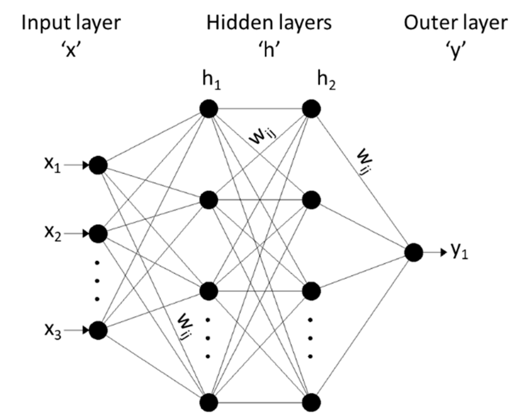
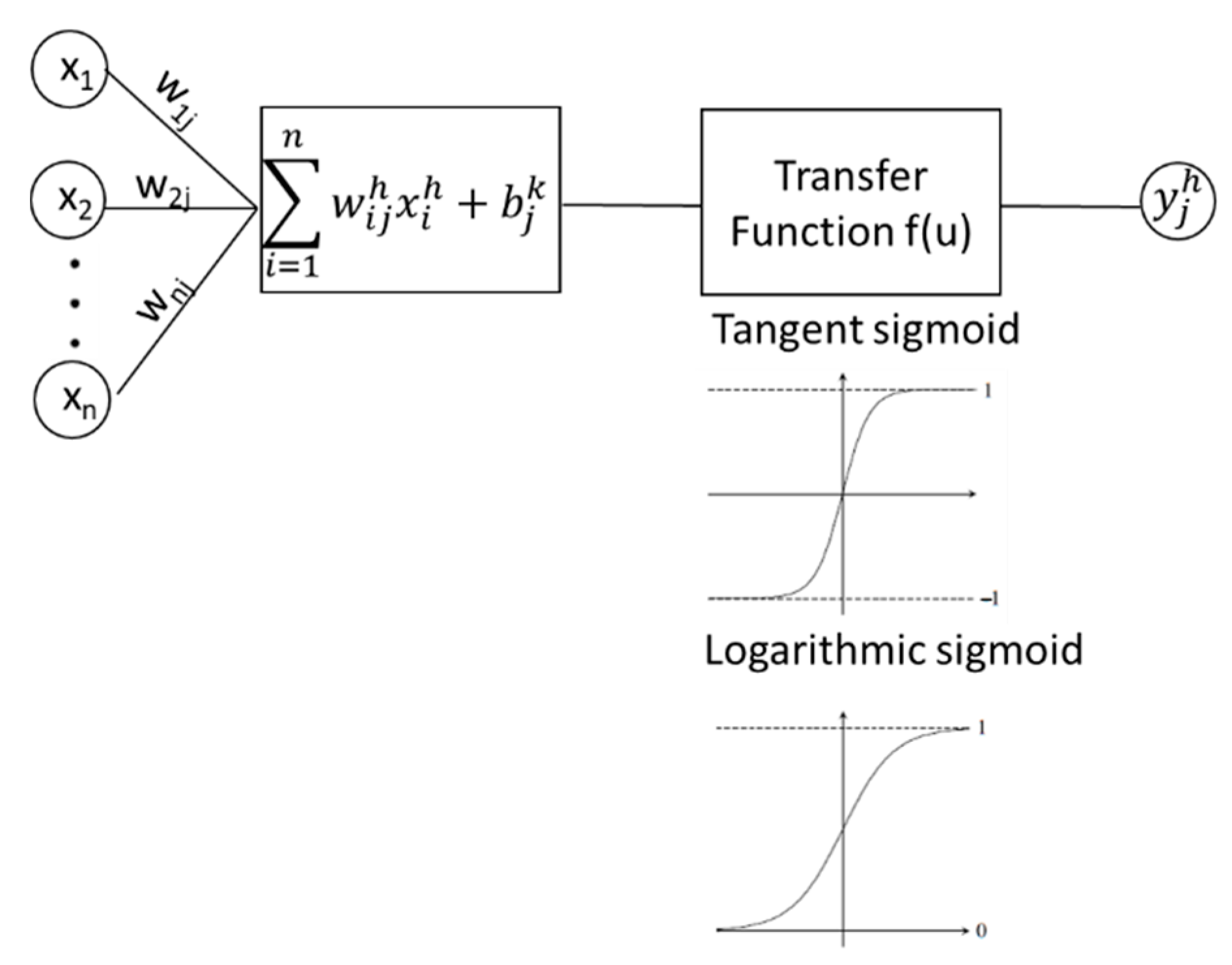
2.1. Artificial Neural Network (ANN)

The concept of ANN is derived from biological sciences, where it mimics the complexity of the human brain in recognizing patterns through biological neurons, and thus imitates the process of thinking, recognizing, making decisions, and solving problems [42,43]. ANN was the most popular method found in the reviewed literature to predict wind-induced pressures compared to other neural network methods (e.g., CNN or RNN). ANN is robust enough to solve multivariate and nonlinear modeling problems, such as classification and predictions. ANN is a group of layers that comprise multiple neurons at each layer and is also known as a feed-forward neural network (FFNN). It is composed of input layers, where all the variables are defined and fed into the hidden layers which are weighted and fed into the output layers that represent the response of the operation. The ANN architecture could be written as x-h-h-y which defines x number of inputs (variables), h number of hidden layers, and y number of outputs (responses) as shown in Figure 1. Each hidden layer comprises a certain number of neurons that gives a robust model, and this could be achieved by training and trials.
The hidden layers are composed of activation functions that apply different weights to the input layer and transfer them to the output layers. The most common activation functions are the nonlinear continuous sigmoid, the tangent sigmoid, and the logarithmic sigmoid [44]. The weights are multiplied with the inputs and calibrated through a training process between the input and output layers to reduce the loss. The training process is applied using the Levenberg–Marquardt backpropagation algorithm, which belongs to the family of the Multi-Layer Perceptron (MLP) network [45] and was originally proposed by Rumelhart et al. [46]. It consists of two steps: feed-forward the values to calculate the error, and then propagate back the error to previous layers [47,48]. The repeated iteration process (epochs) of backpropagation network error continues and it keeps adjusting the interconnecting weights until the network error is reduced to an acceptable level. Once the most accurate solution is formed during the training process, the weights and biases are fixed, and the training process stops. The Levenberg–Marquardt is a standard numerical method which achieves the second-order training speed with no need to compute the Hessian matrix and was demonstrated to be efficient with training networks up to a few hundred weights [47,49]. Figure 2 shows the output signal for a generic neuron j in the hidden layer h defined in Equation (1), where w i j h is the weight that connects the ith neuron of the current layer to the jth neuron of the following layer, xi is the input variable, b is the bias associated with the jth neuron to adjust the output along with the weighted sum, and f is the activation function that is usually adapted as either a tangent sigmoid or a logarithmic sigmoid, Equations (2) and (3), respectively. The (RBF-NN) that was used first by [50] is a function whose response either decreases or increases with the distance from a center point [51,52].
y j h = f   ( i = 1 n w i j h x i h + b j k )
f   ( u ) = 1 + 2 ( 1 + e 2 u )
f   ( u ) = 1 ( 1 + e u )
During the training process of BPNN, usually, the training is terminated when one of the following criteria is first met: (i) fixing the number of epochs to a certain number, (ii) the training error is less than a specific training goal, or (iii) the magnitude of the training gradient is less than a specified small value (i.e., 1.0 × 10⁻¹⁰). The training error is the error obtained from running the trained model back on the data used in the training process, while the training gradient is the error calculated as a direction and magnitude during the training of the network that is used to update the network weight in the right direction and amount.

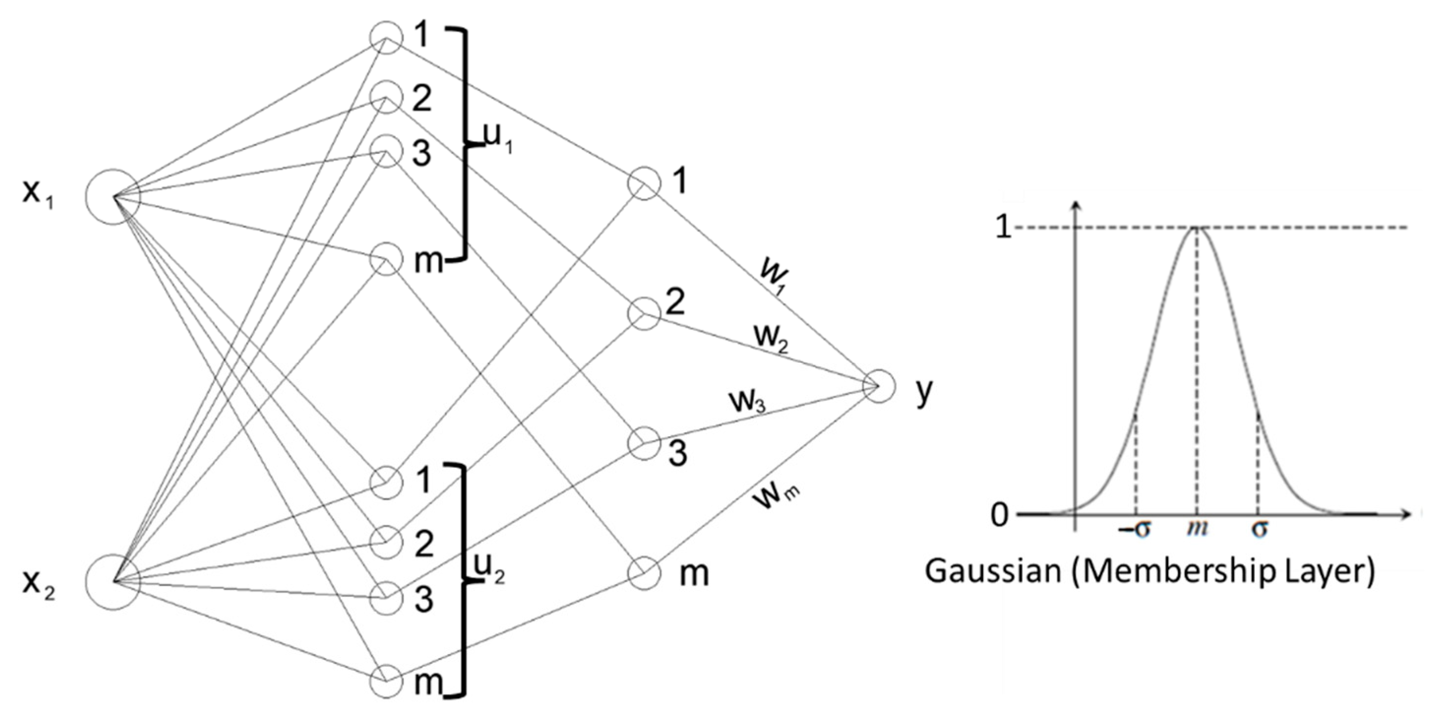
2.2. Fuzzy Neural Network (FNN)

The FNN approach combines the capability of neural networks with fuzzy logic reasoning attributes [53,54]. The architecture of FNN is composed of an input layer, a membership layer, an inference layer, and an output layer (defuzzification layer), as shown in Figure 3. The membership and inference layers replace the hidden layers in the ANN. The input layer consists of n number of variables and the inference layer is composed of m number of rules, and accordingly n × m numbers of neurons exist in the membership layer. The activation function adopted in the membership layer is a Gaussian function as shown in Equation (4) and illustrated in Figure 3.
u i j = exp ( ( x i m i j ) 2 σ i j 2 ) ,   1   i     n ,   1     j     m
where uij is the value of the membership function of the ith input corresponding to the jth rule, mij and σij are the mean and the standard deviation of the Gaussian function.

2.3. Decision Tree (DT)

The DT method is one of the supervised ML models where the algorithm assigns the output through testing in a tree of nodes and by filtering the nodes (decision nodes) down within the split sub-nodes (leaf nodes) to reach the final output. The decision trees may differ in several dimensions such as the test might be multivariate or univariate, or the test may have two or more outcomes, and the attributes might be numeric or categorical [55,56,57].

2.4. Ensemble Methods (EM)

The EM methods include: (1) bagging regression tree that is also referred to as the random forest (RF) algorithm, (2) gradient boosting regression tree (GBRT) or decision tree (GBDT), and (3) extreme gradient boosting (XGB). All EM methods could be defined as a combination of different decision trees to overcome the weakness that may occur in a single tree such as sensitivity to training data and unstableness [58]. The forest generated by the RF algorithm is either trained through bagging, which was proposed by Breiman [59], or through bootstrap aggregating [60]. RF splits in each node n features among the total m features, where n is recommended to be 1 3 m or 2 m [61]. It reduces the overfitting of datasets and increases precision. Overfitting is overtraining the model which causes it to be particular to certain datasets and lose the generalized aspect desired in ML models. The DR and RF methods are commonly used in classification and regression problems.
GBRT, also known as GBDT as mentioned above, was first developed by Friedman [62] and is one of the most powerful ML techniques deemed successful in a broad range of applications [63,64]. GBDT combines a set of weak learners called classification and regression tree (CART). To eliminate overfitting, each regression tree is scaled by a factor, called learning rate (Lr) which represents the contribution of each tree to the predicted values for the final model. The predicted values are computed as the sum of all trees multiplied by the learning rate [65]. Lr with maximum tree depth (Td) determines the number of regression trees for building the model [66]. Previous studies proved that smaller Lr decreases the test error but increases computational time [63,64,67]. A subsampling procedure was introduced by Friedman [60] to improve the generation capability of the model using subsampling fraction (Fs) that is chosen randomly from the full date set to fit the base learner.
Another popular method from the EM family is the XGBoost, or XGB as defined above, which is similar to the random forest and was developed by Chen and Guestrin [68]. XGB has more enhancement compared to other ensemble methods. It can penalize more complex models by using both LASSO (L1) and Ridge (L2) regularization to avoid overfitting. It handles different types of sparsity patterns in the data, and it uses the distributed weighted quantile sketch algorithm to find split points among weighted datasets. There is no need to specify in every single run the exact number of iterations as the algorithm has built-in cross-validation that takes care of this task.

2.5. Gaussian Process Regression (GPR)

The GPR is a supervised learning model that combines two processes: (1) prior process, where the random variables are collected, and (2) posteriori process, where the results are interpolated. This method was introduced by Rasmussen [69] and developed on the basis of statistical and Bayesian theory. GPR has a stronger generalization ability, self-calculates the hyper-parameters in GPR, and the outputs have clear probabilistic meaning [70]. These advantages make the GPR preferable compared to BPNN, as it could handle complex regression problems with high dimensions and a small sample size [69,71]. Background theory and informative equations can be found in detail in the literature [69,70].

2.6. Generative Adversarial Networks (GAN)

The GAN technique was proposed by Goodfellow et al. [72], which is based on a game theory of a minimax two players game. The GAN has attracted worldwide interest in terms of generative modeling tasks. The purpose of this approach is to estimate the generative models via an adversarial process. The approach is achieved by training two models; first, a generative model G that capture all the distribution in the data, and second, a discriminative model D that estimates the probability of a sample to come from the training data rather than G. The G model defines the p model (x) and draws samples from the distribution of p model. The input is placed as vector z and the model is defined by a prior distribution p(z) over the vector z as a generator function G(z:θ(G)), where θ(G) is a set of learnable parameters that define the generator’s strategy in the game [73]. More details about the GAN models can be found in [72,73].

2.7. K-Nearest Neighbors (KNN)

The KNN algorithm is a supervised non-parametric classification machine learning algorithm that was developed by Fix and Hodges [74]. The KNN does not perform any training or assumption for storing the data, but it assigns the unseen data to the nearest set of data used in the training process. According to the value of K, the algorithm started to determine the class for the point to be assigned to according to the value K. For instance, if K is 1, the unseen point will be assigned to a certain class according to the class of the nearest point, or to the nearest five points in the case of K is 5, etc. The KNN is one of the simplest ML classification algorithms and more details can be found in [75].

2.8. Support Vector Machine (SVM)

The SVM is a supervised learning method used for the purpose of classification and regression that use kernel functions. The SVM algorithm is based on determining a hyperplane in an N-dimensional space depending on the number of features that classify the dataset. The optimum hyperplane for classification purposes is associated with the maximum margin between the support vectors which are composed of the dataset nearest to that hyperplane [76]. SVM was developed by Vapnik [77] and is considered to be one of the most simple and robust classification algorithms. More details about SVM can be found in [78].

3. Prior Studies on Applying ML Techniques in Structural Wind Engineering

A broad range of studies is summarized in this section based on the three categories mentioned before, i.e., (1) prediction of wind-induced pressure/speed on different structures using data from experimental models, (2) integration of CFD models with ML models for wind loads prediction, and (3) assessment of the aeroelastic responses for buildings and bridges. Like several ML trends, the number of studies applying or implementing ML for wind engineering has been increasing significantly, specifically in the last couple of years. This reveals the future potential within the wind engineering community where ML techniques continue to gain more attention and interest from academicians and researchers. More than 50% of the total number of studies that were considered in this survey and started in the past 30 years were published only in the last two years (Figure 4), which elucidates the importance of implementing ML techniques in this important and critical domain.

3.1. Prediction of Wind-Induced Pressure

Wind-induced pressure prediction forms an essential area in structural wind engineering. In addition to field studies, different tools can be used for estimating wind loads and pressure coefficients on surfaces, such as atmospheric boundary layer wind tunnels (ABLWT) or CFD simulations. Both ABLWT and CFD are commonly used but in some cases may require significant time, cost and expertise [79]. As in other fields of civil engineering, studies using ML techniques have gained some momentum and wind engineers have shown interest in identifying a reliable approach to predict wind speeds and or wind-induced pressures for common wind-related structural applications. A summary of the key attributes and ML implementation in the studies that were included in the review related to the first category, i.e., the prediction of wind-induced pressures and time series from experimental testing or databases, is first provided in Table 1, then each study is discussed in more details in this section. The input variables used in each study are significant to the desired output needed from training the ML model. It depends mainly on the architecture of the model and the different inclusive parameters for each dataset. For predicting surface pressure it may depend mainly on either the coordinates of the pressure taps, or slope of the roof, wind direction, or building height. While for the aeroelastic responses of bridges, the input variables mainly depend on parameters such as displacement, velocity and acceleration response for the bridges. One of the studies used the dimension between the buildings as input variables (Sx, Sy) to predict the interference effect on surface pressure.
Many methods can be used for predicting and interpolating multivariate modeling problems, such as linear interpolation and regression polynomials. However, linear interpolation cannot solve nonlinear problems and regression polynomials are common to obtain empirical equations, but these empirical equations lack the generality to be used with other data and a large number of variables [81]. Therefore, ML models generally and ANN particularly have the advantages over the latter methods in complex problems.
Most of the studies have adopted the three-stage evaluation process of training, testing and validation (TTV), which was proposed by [93] to build a robust ML model. The cross-validation process comprises two steps: first, the dataset is randomly shuffled and is divided into k subsets of similar sizes, then k − 1 sets are used for training and one set is used as the testing set to assess the performance of the model. The stability and the accuracy of the validation method depend mainly on the k value. Hence, the cross-validation method is usually referred to as k-fold cross-validation [19,94] and is illustrated in Figure 5. Many of the reviewed studies used the 10-fold CV method following Refaeilzadeh et al.’s [95] recommendation of using k = 10 as a good estimate.
ANN is the most commonly used technique employed in the reviewed studies (see Table 1). A study by Chen et al. [81] predicted the pressure coefficients on a gable roof using ANN. This was one of the most important and early studies for implementing ML models to predict wind-induced pressure on building surfaces. Later, Chen et al. [96] interpolated pressure time series from existing buildings to different roof height buildings, and then successfully extrapolated to other buildings with different dimensions and roof slopes using ANN.
Zhang and Zhang [82] evaluated the interference wind-induced effects, that were expressed by interference factor (IF) among tall buildings using radial basis function neural networks (RBF-NN). The RBF-NN is a feed-forward type neural network, but the activation function is different from those that are commonly used (i.e., tangent sigmoid or a logarithmic sigmoid). The RBF-NN was used first by [50] and it is a function whose response either decreases or increases with the distance from a center point [51,52]. It was found that the predicted IF values were in very good agreement with the experimental counterparts. The interference index due to shielding between buildings was predicted from experimental data from wind tunnels using neural network models by English [97]. The study found that the neural network model was able to accurately predict the interference index for building configurations that have not been tested experimentally. The interference index can be calculated by subtracting 1 from the shielding (buffeting) factor.
Bre et al. [85] predicted the surface-averaged pressure coefficients of low-rise buildings with different types of roofs using ANN. The predicted mean pressure coefficients, using the Tokyo Polytechnic University (TPU) database [98] as input data, were reasonable when compared to the “M&P” parametric equation [99] and the “S&C” equation [100]. Those two equations are provided here (Equations (5) and (6), respectively) for convenience.
C p ¯ ( θ , D B ) = a 0 + a 1 G + a 2 θ + a 3   θ 2 + a 4 G θ 1 + b 1 G + b 2 θ + b 3   θ 2 + b 4 G θ
C p ¯ ( θ , D B ) = C p ( 0 ° ) ¯   ln [ 1.248 0.703 sin ( θ 2 ) 1.175   sin 2 ( θ ) + 0.131 sin 3 ( 2 G θ ) + 0.769 cos ( θ 2 ) + 0.07 G 2 sin 2 ( θ 2 ) + 0.717 cos 2 ( θ 2 ) .  
where ai and bi are adjustable coefficients, θ is the wind angle, D/b is the side ratio, G = ln(D/B), and C p ( 0 ° ) ¯ is assumed by Swami and Chnadra [100] equal to 0.6 independent from D/B.
Hu and Kwok [66] successfully predicted the wind pressures around cylinders using different ML techniques for Reynolds numbers ranging from 104 to 106, and turbulence intensities levels ranging from 0% to 15% using several data from previous literature. In this particular study, the RF and GBRT performed better than the single regression tree model. Fernández-Cabán et al. [86] used ANN to predict the mean, RMS and peak pressure coefficients on low-rise building flat roofs for three different scaled models. The predicted mean and RMS pressure coefficient show a very good agreement with the experimental data, especially for the smaller-scale model. Hu and Kwok [88] investigated the wind pressure on tall buildings under interference effects using different ML models. The models were trained by different portions of the dataset ranging from 10% to 90% of the available data. The results showed that the GANs model could predict wind pressures based on 30% training data only, which may eliminate 70% of the wind tunnel test cases and accordingly decrease the cost of testing. In addition, RF exhibited a good performance when the number of grown trees, the n number of features and the maximum depth of the tree were set to 100, 3 and 25, respectively. Likewise, Vrachimi [101] predicted wind pressure coefficients for box-shaped obstructed building facades using ANN with a ±0.05 confidence interval for a confidence level of 95%.
Tian et al. [90] focused on predicting the mean and the peak pressure coefficient on a low-rise gable building using a deep neural network (DNN). This study presented a strategy to predict peak pressure coefficients which is considered a more challenging task when ML models are used. The strategy is used to predict first the mean pressure coefficient and then use the predicted mean pressure as an input with other input variables to predict peak pressure coefficients. This strategy is a reflection of the ensemble methods idea [58], which is an effective method for solving complex problems with limited inputs. FNN models were also successfully used in several studies [53,54,102] to predict mean pressure distribution and power spectra of fluctuating pressures. The most significant feature of FNN models is the capability of approximating any nonlinear continuous function to a desired degree of accuracy. Thus, this family of methods can capture the non-linearity relationship between the different input variables such as wind pressures, wind directions, and coordinates of pressure taps.
Another technique that is based on the methodology of applying ANN was used by Mallick et al. [92] in predicting surface mean pressure coefficients using equations for the group method of data handling neural networks (GMDH-NN)—a derivative method from ANN. The GMDH-NN is a self-organized system that provides a parametric equation to predict the output and can solve extremely complex problems [103]. This ML algorithm was established using the GMDH shell software [104] and it is based on the principle of termination [104,105,106] to find the nonlinear relation between pressure coefficients and the input variables. Termination is the process where the parameters are seeded, reared, hybridized, selected, and rejected to determine the input variables. The study investigated in detail the effect of curvature and corners on pressure distribution and obtained an equation with different variables to predict the mean pressure coefficients. One major difference between ANN and GMDH-NN is that the neurons are filtered simultaneously based on their ability to predict the desired values, and then only those beneficial neurons are fed forward to be trained in the following layer, while the rest are discarded.
One other method to predict wind-induced pressures and full dynamic response, i.e., time history on high-rise building surfaces, was proposed by Dongmei et al. [84] using a backpropagation neural network (BPNN) combined with proper orthogonal decomposition (POD-BPNN). POD was utilized by Armitt [107] and later by Lumley [108] to deal with wind turbulence-related issues. The advantage of the POD-BPNN method over the ANN is its capability to predict pressure time series for trained data with time parameter t. POD is an approach that is based on a linear combination of a series of orthogonal load modes, where the spatial distributed multivariable random loads can be reconstructed through it and loading principle coordinates [109]. The orthogonal load modes are space-related and time-independent, while the loading principal coordinates are time-varying and space-independent. Before applying the BPNN, the wind loads were decomposed using POD where the interdependent variables are transformed into a weighted superposition of several independent variables. More details about the POD background theory can be found in the literature [110,111,112]. The training algorithm applied in that study was the improved global Levenberg–Marquardt algorithm, which can achieve a faster convergence speed [113,114]. A similar study by Ma et al. [87] investigated the wind pressure-time history using both gaussian process regression (GPR) and BPNN on a low-rise building with a flat roof. The study concluded that GPR has high accuracy for time history interpolation and extrapolation.
The wind pressure time series and power spectra were again recently simulated and interpolated on tall buildings by Chen et al. [91] using three ML methods: BPNN, genetic algorithm (GANN), and wavelet neural network (WNN). The WNN produced the most accurate results within the three methods. The WNN combines the advantages of ANN with wavelet transformation, which has time-frequency localization property and focal features which are different from neural networks that have self-adaptive, fault tolerance, robustness and strong inference ability [115]. The reviewed literature showed that the developed BPNN models could generalize the complex, multivariate nonlinear functional relationships among different variables such as wind-induced pressures and locations of pressure taps. Predicting pressure time series at different roof locations was achieved using ANN and the robustness of the models was able to overcome the problems associated with linear interpolation for low-resolution data.
A recent study [92] developed an ML model to predict the wind-induced mean and peak pressure for non-isolated buildings, considering the interference effect of neighboring structures using GBDT combined with the grid search algorithm (GSA). The study used wind tunnel data from TPU for non-isolated buildings. The data were split by a ratio of 9:1, where 90% of the dataset was used for training and 10% of the dataset was used for testing. Four hyperparameters were considered in developing the ML model, two hyperparameters for CART (i.e., maximum depth, d, for each decision tree, and a minimum number of samples to split an internal node), and two hyperparameters for a gradient boosting approach, i.e., learning rate (Lr) and number of CART models. The developed method was shown to be a robust and accurate method to predict the wind-induced pressure on structures under the interference effects of neighboring structures. Zhang et al. [116] predicted the typhoon-induced response (TIR) on long-span bridges using quantile random forest (QRF) with bayesian optimization instead of the traditional FE analysis. The QRF with bayesian optimization was able to provide adequate probabilistic estimations to quantify the uncertainty in predictions.

3.2. Integration of CFD with Machine Learning

Several studies integrated CFD simulations with ML techniques to predict either the wind force exerted on bluff bodies or the aeroelastic response of bridges and other flexible structures [117,118,119,120,121,122]. Chang et al. [123] predicted the peak pressure coefficients on a low-rise building using 12 output data types from a CFD model such as mean pressure coefficient, dynamic pressure, wind speed, etc. as input variables in the ANN model. The predicted peak pressures were in good agreement with the wind tunnel data. Similarly, Vesmawala et al. [124] used ANN to predict the pressure coefficient on domes of different span to height ratios. The data were generated from the CFD model by developing a dome and a wind flow through the model. The predicted mean pressure coefficients were used for training the ML model with a maximum number of epochs of 50,000 to achieve the specified error tolerance. There were three main inputs: the span/height ratio, the angle measured vertically with respect to the vertical axis of the dome to the ring beam, and the angle measured horizontally with respect to wind direction. The study used neuroscience software in the model training and testing, and it was found that the BPNN predicted the mean pressure coefficients accurately through different locations along the dome.
Bairagi and Dalui [125] investigated the effect of a setback in tall buildings by predicting pressure coefficients along the building’s face. The study used ANN and Fast Fourier Transform (FFT) to validate the wind-induced pressure on different setback buildings predicted by CFD simulation models. The predicted wind pressures were validated before using similar experimental data. The study showed that CFD was capable to predict similar pressure coefficients to experimental data and showed that ANN was capable to predict and validate these pressure coefficients. The Levenberg–Marquardt algorithm was used as the training function, starting with 500 training epochs which were increased until the correlation coefficient exceeded the 99th percentile. The model was trained using MATLAB neural network toolbox [126].
A recent study [127] proposed a multi-fidelity ML approach to predict wind loads on tall buildings by integrating CFD models with ML models. The study combined data from a large number of wind directions using the computationally efficient Reynolds-averaged Navier–Stokes (RANS) model with a smaller number of wind directions using the more computationally intense Large Eddy Simulation (LES) method to predict the RMS pressure coefficients on a tall building. The study utilized four types of ML models: linear regression, quadratic regression, RF, and DNN, with the latter being the most accurate. In addition, a bootstrap algorithm was used to generate an ensemble of ML models with accurate confidence intervals. This study used the Adam optimization algorithm [128] and Rectified Linear Unit (ReLU) activation function [129,130] with a learning rate of 0.001 and regularization strength of 0.01 to avoid overfitting. That was contrary to other studies that used the Levenberg–Marquardt algorithm and tangent sigmoid or logarithmic sigmoid activation functions and this is because the other studies used the ANN method of two or less hidden layers, while the latter study used a DNN with three hidden layers.
To conclude this section, a summary of the attributes of the reviewed previous studies that integrate ML applications with CFD is provided in Table 2.

3.3. Aeroelastic Response Prediction Using ML

The prediction of aeroelastic responses for buildings and structures by using ML models is also of interest to this review. The input that was used for the prediction of these responses is either CFD simulations (Table 2) or physical testing databases (Table 3). Similar to the previous two sections, Table 3 is meant to provide a summary of the attributes of the key studies reviewed in this section that is concerned with using ML for aeroelastic response prediction.
Chen et al. [135] used a BPNN that was built from a limited dataset of already existing dynamic responses of rectangular bridge sections. The results indicated that the ANN prediction scheme performed well in the prediction of dynamic responses. The authors claimed that such an approach may reduce cost and save time by not using extensive wind tunnel testing, especially in the preliminary design. Wu and Kareem [131] developed a new approach utilizing ANN with cellular automata (CA) scheme to model the hysteretic behavior of bridge aerodynamic nonlinearities in the time domain. This approach was developed because the ANN is time-consuming until the ideal number of hidden layers and neurons between the input and output are determined. By embedding the CA scheme, which was originally proposed by [136] and later developed by [137] with ANN, the authors of that study aimed to improve the efficiency of the ANN models. The CA scheme is an approach that dynamically evolves in discrete space and time using a local rule belonging to a class of Boolean functions. This scheme is appealing as it could simulate very complicated problems with the simple local rule which is applied to the system consistently in space and time. The activation function used in the ANN training was bipolar sigmoid as shown in Equation (7). The CA scheme is an indirect encoding scheme that is based on the CA representative and could be designed using two cellular systems, i.e., the growing cellular system and the pruning cellular system [138]. The ANN configuration based on the CA scheme was examined using a fitness index that is defined in Equation (8), which is a function of learning cycles and connections of ANN [139].
f   ( u ) = 2 1 + exp ( u ) 1
f i = 1 ( c o n n i j + c o n n j k ) c y c
Table 3. Summary of studies reviewed for aeroelastic response.
Study No.Ref.Surface TypeSource of DataInput VariablesOutput VariablesML Algorithm
1[135]BridgesExperimental data from BLWTD/BFlutter derivatives
(H1 and A2)
ANN
2[140]Tall buildingsExperimental data from BLWTVb and top floor displacementsColumn strainsCNN
3[141]Tall buildingsIndianWind CodeH, B, L, Vb and TCAcross wind shear and momentANN
4[142]Long span bridgeFull scale dataCross spectral densityBuffeting responseANN and SVR
5[143]Box girdersExperimental data from BLWTVertex coordinates (mi, ni)Flutter wind speedSVR, ANN, RF and GBRT
6[144]Rectangular cylindersPrevious experimental studiesTi, B/D and ScCrosswind vibrationsDT-RF-KNN-GBRT
7[145]Cable roofsExperimental data from BLWT and (FEM)11 parametersVertical displacementsANN
8[146]Tall buildingsWERC database-TUTerrain roughness, aspect ratio and D/B.Crosswind force spectraLGBM
The dynamic response of tall buildings was studied by Nikose and Sonparote [141,147] using ANN and the proposed graphs were able to predict the along- and across-wind responses in terms of base shear and base bending moments according to the Indian Wind Code (IWC). Both studies found that the back propagation neural network algorithm was able to satisfactory estimate the dynamic along- and across-wind responses of tall buildings. Similarly, different ML models were applied by Hu and Kwok [144] based on DT, KNN regression, RF, and GBRT to predict four types of crosswind vibrations (i.e., over-coupled, coupled, semi-coupled and decoupled) for rectangular cylinders. The data used in training and testing processes were extracted from wind tunnel data. It was found that GBRT can accurately predict crosswind responses which can supplement wind tunnel tests and numerical simulation techniques. One of the input variables used in that study was the Scruton number (Sc).
Oh et al. (2019) [140] studied the wind-induced response of tall buildings using CNN and focused on the structural safety evaluation. The trained model predicted the column strains using wind tunnel data such as wind speed and top floor displacements. The architecture of the trained model is composed of the input layer, two convolutional layers, two pooling layers, one fully connected layer, and the output layer. The input map forms the convolutional layer through convolution using the kernel operator. The ML-based model was utilized to overcome the uncertainties in the material, geometric properties and stiffness contribution of nonstructural elements which make it difficult to construct a refined finite element model.
Li et al. [133] used LSTM—originally proposed by Hochreiter and Schmidhuber [148]—to predict the nonlinear unsteady bridge aerodynamic responses to overcome the increasing difficulties that exist in the gradient-based learning algorithm in the recurrent neural network (RNN) face. The RNN was developed to introduce the time dimension into the network structure, and it was found to be capable of predicting a full-time series where nonlinear relation exists between input and output. The study used displacement time series as input variables, and by weighting these time series, both the acceleration and velocity were obtained. The LSTM model was able to calculate the deck vibrations (i.e., lift displacement and torsional angle) under the unsteady nonlinear wind loads. Hu and Kwok [136] investigated the vortex-induced vibrations (VIV) of two circular cylinders with the same dimensions but staggered configurations, using three ML algorithms: DT, RF, and GBRT. The two cylinders were modeled first into a CFD simulation, and the mass ratio, wind direction, the distance between cylinders, and wind velocity were used as input variables. The GBRT algorithm was the most accurate in predicting the amplitude of the upstream and downstream vibration. Abbas et al. [132] employed ANN to predict the aeroelastic response of bridge decks using response time histories as the input variables. The predicted forces were compared with CFD findings to evaluate the ANN model. The ANN model was also coupled with the structural model to determine the aeroelastic instability limit of the bridge section, which demonstrated the potential use of this framework to predict the aeroelastic response for other bridge cross-sections.
More recently, surrogate models have been used widely in different areas related to structural wind engineering [149,150,151,152]. One type of surrogate model is using the aid of finite element models (FEM) to obtain an output that can be used as an input in the trained model of the ML. Chen et al. [153] used a surrogate model in which the ANN was applied to the FE model to update the model parameter for computing the dynamic response of a cable-suspended roof while using the wind loads from full-scale measurements for three typhoon events in three consecutive years from 2011 to 2014. Luo and Kareem [154] proposed a surrogate model using a convolutional neural network (CNN) for systems with high dimensional inputs/outputs. Rizzo and Caracoglia [145] predicted the wind-induced vertical displacement of a cable net roof using ANN. The trained model used wind tunnel pressure coefficient datasets and FEM wind-induced vertical displacement datasets. The surrogate model showed that it can successfully replicate more complex geometrically nonlinear structural behavior. Rizzo and Caracoglia [155] used surrogate flutter derivate models to predict the flutter velocity of a suspension bridge. The ANN model was trained using the critical flutter velocities dataset by calculating the flutter derivatives experimentally. The model successfully generated a large dataset of critical flutter velocities. In addition, surrogate modeling could analyze the structural performance of vertical structures under tornado loads by training fragilities using ANN [156,157].
Lin et al. [146] used a light gradient boosting machine (LGBM) method, which is an optimized version of the GBDT algorithm proposed by Ke et al. [158], with a clustering algorithm to predict the crosswind force spectra of tall buildings. This optimized algorithm combined two techniques in training the models: the gradient base one side sampling (GOSS) and the exclusive feature bundling (EFB). The results showed that the proposed method is effective and efficient to predict the crosswind force spectrum for a rectangular tall building.
Liao et al. [143] used four different ML techniques (i.e., SVR, ANN, RF, and GBRT) to predict the flutter wind speed for a box girder bridge. The ANN and GBRT models accurately predicted the flutter wind speed for the streamlined box girders. The buffeting response of bridges can be predicted analytically using buffeting theory. However, some previous studies [159,160,161,162,163] have shown inconsistency between full-scale measured response and buffeting theory estimates. Thus, Castellon et al. [142] trained two ML models (ANN and SVR) to estimate the buffeting response speed using full-scale data from the Hardanger bridge in Norway. The two ML models predicted the bridge response more accurately than the buffeting theory when compared to the full-scale measurement. Furthermore, the drag force of a circular cylinder can be reduced by optimizing the control parameter such as feedback gain and the phase lag using neural networks by minimizing the velocity fluctuations in the cylinder wake [164].

4. Summary of Tools of Performance Assessment of ML Models

The performance of the ML models in wind engineering applications throughout the reviewed literature was assessed through at least one or more forms of different standard statistical error and standard indices. It is important for any ML model to evaluate the performance of the model using some error metrics or factors. Thus, this section aims to provide future researchers with a summary of all the tools and equations that have been used up to this date in structural wind engineering ML applications along with an assessment of which tools are more appropriate for the applications at hand. The compiled list of metrics, or factors, calculates the error to evaluate the accuracy between the ML predicted data and a form of ground truth such as experimental data or independent sets of data that were not used in training among others. There is always a lack of consensus on the most accurate metric that can be used. Nonetheless, this section attempts to provide more guidance on which methods are preferred based on the surveyed studies.
Several error metrics were used throughout the reviewed literature which include: Akaike information criterion (AIC), coefficient of efficiency (Ef), coefficient of determination (R2), Pearson’s correlation coefficient (R), mean absolute error (MAE), mean absolute percentage error (MAPE), mean square error (MSE), root mean square error (RMSE), scatter index (SI), and sensitivity error (Si). For the convenience of the readers and for completeness, the equations used to express each of these error metrics for assessing predicted data (pi) against measured data (mi) are summarized below (Equations (9)–(18)). For N number of data points (e.g., N could be the number of pressure tabs used to provide experimental data), some of the error calculation equations also use average or mean values for predicted data ( p ¯ ) as well as measured data ( m ¯ ).
A I C = N   log ( 1 N i N ( p i m i ) 2 ) + 2 k
E f = 1 i N | m i p i | i N p i
R 2 = i N ( m i m ¯ ) ( p i p ¯ )   i N ( m i m ¯ ) 2 i N ( p i p ¯ ) 2
R = i N ( m i m ¯ ) ( p i p ¯ )   i N ( m i m ¯ ) 2 i N ( p i p ¯ ) 2
M A E = 1 N   i N | m i p i |
M A P E = 1 N i N ( p i m i p i ) × 100 %
M S E = 1 N i N ( p i m i m i ) 2  
R M S E = 1 N i N ( p i m i ) 2  
S I = i N [ ( p i p ¯   ) ( m i m ¯ ) ] 2 i N ( m i ) 2
S i = X i i = 1 n X i × 100 ;   where   X i = f m a x   ( x i ) f m i n   ( x i ) ,
where f m a x   ( x i   )   and   f m i n   ( x i ) , are the corresponding maximum and minimum values for the predicted output over the ith input factor while using the mean values for the other factors.
In general, MSE was employed in most of the studies and is considered one of the most common error metrics for pressure distribution prediction, but it is not always an accurate error metric. The MSE accuracy decreases when the pressure among the walls is included in the prediction because walls might introduce a pressure coefficient near zero which may cause a great rise as the normalizing denominator [90]. Nevertheless, MSE is generally stable when used in RF models when the number of trees reaches 100 [88]. The RMSE is not affected by the near-zero pressure coefficient as with MSE because it does not include a normalization factor in the calculation. Nevertheless, the lack of normalization is considered a limitation for this metric in the cases where the scale of pressure coefficients changes [90]. The accuracy of some metric errors increases when their values approach one (i.e., coefficient of determination-R2), which means that the predicted data are close to the experimental data, and the accuracy of some others increases when their values are close to zero (i.e., root mean square error-RMSE).
The correlation coefficient, R, is considered a reliable approach for estimating the prediction accuracy by measuring how similar two sets of data are, but its limitation is that it does not reflect the range nor the bias between the two datasets. The coefficient of efficiency, E, corresponds to the match between the model and observed data and can range from −∞ to 1, and a perfect match corresponds to E = 1 [89]. AIC is a mathematical method used to evaluate how the model fits the trained data and this is an information criterion used to select the best-fit model. One other error metric that has not been commonly used in the literature is the SI normalized measure of error, where a lower SI value indicates better performance for the model. Besides the error metrics that assess the performance level of the model, other factors are used to indicate the effect of input variables on the output. The most common example is the sensitivity analysis error percentage (Si) (Equation (18)) which computes the contribution of each input variable to the output variable [165,166,167]. The Si is an important factor to determine the contribution of each input value, especially when different inputs are used in the ML model training, which could be of great significance for informing and changing the assigned weight of neurons in neural networks.
Overall, it is important to note that each error metric or factor usually conveys specific information regarding the performance of the ML model, especially in the case of wind engineering applications (due to variation of wall versus roof pressures for instance), and most of these metrics and factors are interdependent. Thus, our recommendation is to consider the following factors together: (1) use R2 to assess the similarity between the actual and predicted set; (2) use MSE when the model includes the prediction of roof surface pressure coefficients only without walls, but use either MAPE or RMSE when pressure coefficients for walls’ surfaces are included in the model; (3) use AIC to select the best fit model in case of linear regression. This recommendation is to stress the fact that using several metric errors together is essential to assess the performance of ML models for structural wind engineering as opposed to only relying on a single metric.

5. Discussion and Conclusions

As in any other application, the quantity and the quality of data is the main challenge in successfully implementing ML models in the broader area of structural wind engineering. It is important to mention that the quality of the dataset used for training is as important as the quantity of data. The measurements usually may involve some anomalies such as missing data or outliers, thus removing the outliers is essential for the accuracy and robustness of the model [168,169]. ML algorithms are data-hungry processes that require thousands if not millions of observations to reach acceptable performance levels. Bias in data collection is another major drawback that could dramatically affect the performance of ML models [170]. To this end, some literature recommends that the number of datasets shall not be taken less than 10 times the number of independent variables, according to 10 events per variable (EPV) [171]. Meanwhile, K-means clustering was used in many different studies due to its ability to analyze the dataset and recognize its underlying pattern. Most of the ML techniques need several trials and experiments through the validation process to develop a robust model with high accuracy prediction levels. For instance, whenever ANN is used, several trials are conducted for training purposes in terms of choosing the number of hidden layers and the number of neurons in each layer.
The ANN method is not recommended for datasets with a small sample size because this would achieve double the mean absolute error (MAE) compared to other ML techniques [134]. ANN is capable of learning and generalizing nonlinear complex functional relationships via the training process, but there is currently no theoretical basis for determining the ideal neural network configuration [81]. The architecture of ANN and training parameters cannot be generalized even within data of similar nature [141]. Generally, one hidden layer is enough for most problems, but for very complex, fuzzy and highly non-linear problems, more than one hidden layer (node) might be required to capture the significant features in the data [172]. The number of hidden nodes is determined through trials and in most cases, this number is set to no more than 2n + 1, where n is the number of input variables [173]. In addition, a study by Sheela and Deepa [174] reviewed different models for calculating the number of hidden neurons and developed a proposed method that gave the least MSE compared to the other models. The proposed approach was implemented on wind speed prediction and was very effective compared to other models. Furthermore, a general principle of a ratio of 3:1 or 3:2 between the first and second hidden nodes provides a better prediction performance compared to other combinations [175]. Generally, a robust neural network model can be built of two hidden layers and ten neurons and will give a very reasonable response.
ANN also appears to have a significant computational advantage over a CFD-based scheme. In ANN, the computational work is mainly focused on identifying the proper weights in the network. Once the training phase is completed, the output of the simulated system could be obtained through a simple arithmetic operation with any desired input information. On the other hand, in the case of a CFD scheme, each new input scenario requires a complete reevaluation of the fluid–structure interaction over the discretized domain.
From the review of the literature, it was also apparent that ANN has weighted advantages over other ML methods. However, there are some challenges accompanying implementing ANN in certain types of wind engineering applications. ANN is problematic in predicting the pressure coefficients within the leading corner and edges due to the separation which is accompanied by high rms pressure coefficient values and corner vortices. This may be eliminated by training datasets of full- or large-scale models that contain high-resolution pressure tapped areas. It is important to note that whenever the data are fed into a regression model or ANN model (training, validation or testing process), all the predictors are normalized between [−1, 1] to condition the input matrix. In the case of implementing ANN models, the Levenberg–Marquardt algorithm and tangent sigmoid or logarithmic sigmoid activation functions shall be used. On the contrary, the Adam optimization algorithm and Rectified linear unit activation function shall be used whenever a DNN model (i.e., three or more hidden layers) is used as the ML technique.
The literature review revealed that there are selected ML techniques that might not be as popular as ANN yet but with potential for future wind engineering applications and specific structural wind engineering problems. Less common ML methods, such as the wavelet neural network (WNN), are gaining increasing attention due to their advantage over ANN and other models in terms of prediction accuracy and good fit [176]. In addition, wavelet analysis is becoming popular due to its capacity to reveal simultaneous spectral and temporal information within a single signal [177]. Other ML techniques such as DL can be used as a probabilistic model for predictions based on limited and noisy data [178]. GANs models can be used in structural health monitoring for damage detections in buildings using different images for damage that occurred during an extreme wind event. BPNN and GRNN were used to acquire the missing data due to the failed pressure sensors while testing [179]. The GPR has high accuracy for time history interpolation and extrapolation and in the same context, the WNN predicts the time series accurately compared to other methods. Surrogate models were proved to be a powerful tool to integrate both FEM with ML models which could solve complex problems, such as the dynamic response of roofs and bridges while using the wind loads from physical testing measurements and can replicate more complex geometrically nonlinear structure behavior.
Ensemble methods have shown good results in predicting wind-induced forces and vibrations of structures. Due to the time-consuming and cost-prohibitive nature of conducting a lot of wind tunnel testing, ML models such as DT, KNN, RF and GBRT are found to be efficient [144], and in turn, recommended for accurately predicting crosswind vibrations. The GBRT specifically can accurately predict crosswind responses when it is needed to supplement wind tunnel tests and numerical simulation techniques. ANN and GBRT are found to be the ideal ML models for wind speed prediction. Moreover, RF and GBRT are found to predict wind-induced loads more accurately when compared to DT. GBDT is preferable to be used over ANN in the case of a small amount of input data, as ANN requires a large amount of input data for an accurate prediction as explained above. Predicting wind gusts, which has not been a common application in the reviewed work in this study, can be achieved accurately using ensemble methods or neural networks and logistic regression [180,181,182,183,184,185].
If only wind tunnel testing is considered, the wind flow around buildings, which provides deep insight into the aerodynamic behavior of buildings, is usually captured using particle image velocimetry (PIV). However, measuring wind velocities at some locations is a challenge due to the laser-light shielding. In such cases, DL might be used to predict these unmeasured velocities at certain locations as proposed in previous work [186]. Tropical cyclones and typhoons’ wind fields can be predicted using ML models using the storm parameters such as spatial coordinates, storm size and intensity [187,188].
Overall, it was demonstrated through this review that ML techniques offer a powerful tool and were successfully implemented in several areas of research related to structural wind engineering. Such areas that can extend previous work and continue to benefit from ML techniques are mostly: the prediction of wind-induced pressure time series and overall loads as well as the prediction of aeroelastic responses, wind gust estimates, and damage detection following extreme wind events. Nonetheless, other areas that can also benefit from ML but are yet to be explored more and recommended for future wind engineering research include the development and future codification of ML-based wind vulnerability models, advanced testing methods such as cyber-physical testing or hybrid wind simulation by incorporating surrogate and ML models for geometry optimization, wind-structure interaction evaluation, among other future applications. Finally, the physics-informed ML methods could provide a promising way to further improve the performance of traditional ML techniques and finite element analysis.

Author Contributions

Conceptualization, K.M.; methodology, K.M.; validation, K.M., I.Z. and M.A.M.; formal analysis, K.M.; investigation, K.M.; resources, K.M.; writing—original draft preparation, K.M.; writing—review and editing, I.Z. and M.A.M.; supervision, I.Z. and M.A.M. All authors have read and agreed to the published version of the manuscript.

Funding

This research received no external funding.

Institutional Review Board Statement

Not applicable.

Informed Consent Statement

Not applicable.

Conflicts of Interest

The authors declare no conflict of interest.

Abbreviations

Nomenclature
xMachine learning input variable
yMachine learning output
hNeural network hidden layer
x j h Input for a generic neuron
w i j h Weight of a generic connection between two nodes
b j k Bias of a generic neuron
y j h Output for a generic neuron
f ( u ) Transfer function
u i j Value of membership function
mijMean of the Gaussian function
σijStandard deviation of the Gaussian function
L1LASSO regularization
L2Ridge regularization
p i Predicted output
m i Measured output
S i Normalized measure for error
θWind direction
βRoof slope
D/BSide ratio
x, y, zPressure taps coordinates
ReReynolds number
TiTurbulence intensity
Sx, SyInterfering building location
R/DCurvature ratio
d/bSide ratio without curvature
D/HHeight ratio
hBuilding height
ScScruton number
MMass ratio
LDistance between the centerline of the cylinders
UReduced velocity
H1Flutter Derivatives (vertical motion)
A2Flutter Derivatives (torisonal motion)
mi, niVertex coordinates
LLength of the building
VbWind velocity
TCTerrain category
C P ¯ Mean pressure coefficient
C p ˜ Peak pressure coefficient
C ˜ p Root mean square pressure coefficient
φThe angle measured horizontally with respect to wind direction
ПThe angle measured vertically with respect to the vertical axis of the dome to the ring beam.
CANeighboring area density
Abbreviations
ABLWTAtmospheric boundary layer wind tunnel
AICAkaike information criterion
ANNArtificial neural network
CFDComputational fluid dynamics
CNNConvolutional neural networks
DLDeep learning
DNNDeep neural network
DTDecision tree regression
EfCoefficient of efficiency
FFNNFeed-forward neural network
FNNFuzzy neural networks
GANGenerative adversarial networks
GANNGenetic neural networks
GBRTGradient boosting regression tree
GMDH-NNGroup method of data handling neural networks
GPRGaussian process regression
KNNK-nearest neighbor regression
LESLarge eddy simulation
LrLearning Rate
LSTMLong short-term memory
MAEMean absolute error
MAPEMean absolute percentage error
MLMachine learning
MSEMean square error
POD-BPNNProper orthogonal decomposition-backpropagation neural network
RPearson’s correlation coefficient
R2Coefficient of determination
RANSReynolds-averaged Navier–Stokes
RBF-NNRadial basis function neural networks
ReLURectified liner unit
RFRandom forest
RMSRoot mean square
RMSERoot mean square error
RNNrecurrent neural networks
RTHSReal-time hybrid simulation
SIScatter index
SVMSupport vector machine
VIVVortex induced vibration
WNNWavelet neural network

References

  1. Solomonoff, R. The time scale of artificial intelligence: Reflections on social effects. Hum. Syst. Manag. 1985, 5, 149–153. [Google Scholar] [CrossRef] [Green Version]
  2. Mjolsness, E.; DeCoste, D. Machine Learning for Science: State of the Art and Future Prospects. Science 2001, 293, 2051–2055. [Google Scholar] [CrossRef] [PubMed]
  3. Murphy, K.P. Machine Learning: A Probabilistic Perspective; MIT Press: Cambridge, MA, USA, 2012. [Google Scholar]
  4. Sun, H.; Burton, H.V.; Huang, H. Machine learning applications for building structural design and performance assessment: State-of-the-art review. J. Build. Eng. 2020, 33, 101816. [Google Scholar] [CrossRef]
  5. Saravanan, R.; Sujatha, P. A State of Art Techniques on Machine Learning Algorithms: A Perspective of Supervised Learning Approaches in Data Classification. In Proceedings of the 2018 Second International Conference on Intelligent Computing and Control Systems (ICICCS), Madurai, India, 14–15 June 2018; pp. 945–949. [Google Scholar] [CrossRef]
  6. Kang, M.; Jameson, N.J. Machine Learning: Fundamentals. Progn. Health Manag. Electron. 2018, 85–109. [Google Scholar] [CrossRef]
  7. Hastie, T.; Tibshirani, R.; Friedman, J. The Elements of Statistical Learning; Springer Series in Statistics; Springer: Berlin/Heidelberg, Germany, 2001. [Google Scholar]
  8. Adeli, H. Neural Networks in Civil Engineering: 1989–2000. Comput. Civ. Infrastruct. Eng. 2001, 16, 126–142. [Google Scholar] [CrossRef]
  9. Çevik, A.; Kurtoğlu, A.E.; Bilgehan, M.; Gülşan, M.E.; Albegmprli, H.M. Support vector machines in structural engineering: A review. J. Civ. Eng. Manag. 2015, 21, 261–281. [Google Scholar] [CrossRef]
  10. Dibike, Y.B.; Velickov, S.; Solomatine, D. Support vector machines: Review and applications in civil engineering. In Proceedings of the 2nd Joint Workshop on Application of AI in Civil Engineering, Cottbus, Germany, 26–28 March 2000; pp. 45–58. [Google Scholar]
  11. Bas, E.E.; Moustafa, M.A. Real-Time Hybrid Simulation with Deep Learning Computational Substructures: System Validation Using Linear Specimens. Mach. Learn. Knowl. Extr. 2020, 2, 26. [Google Scholar] [CrossRef]
  12. Bas, E.E.; Moustafa, M.A. Communication Development and Verification for Python-Based Machine Learning Models for Real-Time Hybrid Simulation. Front. Built Environ. 2020, 6, 574965. [Google Scholar] [CrossRef]
  13. Xie, Y.; Ebad Sichani, M.; Padgett, J.E.; Desroches, R. The promise of implementing machine learning in earthquake engineering: A state-of-the-art review. Earthq. Spectra 2020, 36, 1769–1801. [Google Scholar] [CrossRef]
  14. Mosavi, A.; Ozturk, P.; Chau, K.-W. Flood Prediction Using Machine Learning Models: Literature Review. Water 2018, 10, 1536. [Google Scholar] [CrossRef] [Green Version]
  15. Munawar, H.S.; Hammad, A.; Ullah, F.; Ali, T.H. After the flood: A novel application of image processing and machine learning for post-flood disaster management. In Proceedings of the 2nd International Conference on Sustainable Development in Civil Engineering (ICSDC 2019), Jamshoro, Pakistan, 5–7 December 2019; pp. 5–7. [Google Scholar]
  16. Deka, P.C. A Primer on Machine Learning Applications in Civil Engineering; CRC Press: Boca Raton, FL, USA, 2019. [Google Scholar] [CrossRef]
  17. Huang, Y.; Li, J.; Fu, J. Review on Application of Artificial Intelligence in Civil Engineering. Comput. Model. Eng. Sci. 2019, 121, 845–875. [Google Scholar] [CrossRef]
  18. Reich, Y. Artificial Intelligence in Bridge Engineering. Comput. Civ. Infrastruct. Eng. 1996, 11, 433–445. [Google Scholar] [CrossRef]
  19. Reich, Y. Machine Learning Techniques for Civil Engineering Problems. Comput. Civ. Infrastruct. Eng. 1997, 12, 295–310. [Google Scholar] [CrossRef]
  20. Lu, P.; Chen, S.; Zheng, Y. Artificial Intelligence in Civil Engineering. Math. Probl. Eng. 2012, 2012, 145974. [Google Scholar] [CrossRef] [Green Version]
  21. Vadyala, S.R.; Betgeri, S.N.; Matthews, D.; John, C. A Review of Physics-based Machine Learning in Civil Engineering. arXiv 2021, arXiv:2110.04600. [Google Scholar] [CrossRef]
  22. Salehi, H.; Burgueño, R. Emerging artificial intelligence methods in structural engineering. Eng. Struct. 2018, 171, 170–189. [Google Scholar] [CrossRef]
  23. Dixon, C.R. The Wind Resistance of Asphalt Roofing Shingles; University of Florida: Gainesville, FL, USA, 2013. [Google Scholar]
  24. Flood, I. Neural Networks in Civil Engineering: A Review. In Civil and Structural Engineering Computing: 2001; Saxe-Coburg Publications: Stirlingshire, UK, 2001; pp. 185–209. [Google Scholar] [CrossRef]
  25. Rao, D.H. Fuzzy Neural Networks. IETE J. Res. 1998, 44, 227–236. [Google Scholar] [CrossRef]
  26. Avci, O.; Abdeljaber, O.; Kiranyaz, S. Structural Damage Detection in Civil Engineering with Machine Learning: Current State of the Art. In Sensors and Instrumentation, Aircraft/Aerospace, Energy Harvesting & Dynamic Environments Testing; Springer: Cham, Switzerland, 2022; pp. 223–229. [Google Scholar] [CrossRef]
  27. Avci, O.; Abdeljaber, O.; Kiranyaz, S.; Hussein, M.; Gabbouj, M.; Inman, D.J. A review of vibration-based damage detection in civil structures: From traditional methods to Machine Learning and Deep Learning applications. Mech. Syst. Signal Process. 2021, 147, 107077. [Google Scholar] [CrossRef]
  28. Hsieh, Y.-A.; Tsai, Y.J. Machine Learning for Crack Detection: Review and Model Performance Comparison. J. Comput. Civ. Eng. 2020, 34, 04020038. [Google Scholar] [CrossRef]
  29. Hou, R.; Xia, Y. Review on the new development of vibration-based damage identification for civil engineering structures: 2010–2019. J. Sound Vib. 2020, 491, 115741. [Google Scholar] [CrossRef]
  30. Flah, M.; Nunez, I.; Ben Chaabene, W.; Nehdi, M.L. Machine Learning Algorithms in Civil Structural Health Monitoring: A Systematic Review. Arch. Comput. Methods Eng. 2020, 28, 2621–2643. [Google Scholar] [CrossRef]
  31. Smarsly, K.; Dragos, K.; Wiggenbrock, J. Machine learning techniques for structural health monitoring. In Proceedings of the 8th European Workshop On Structural Health Monitoring (EWSHM 2016), Bilbao, Spain, 5–8 July 2016; Volume 2, pp. 1522–1531. [Google Scholar]
  32. Mishra, M. Machine learning techniques for structural health monitoring of heritage buildings: A state-of-the-art review and case studies. J. Cult. Heritage 2021, 47, 227–245. [Google Scholar] [CrossRef]
  33. Li, S.; Li, S.; Laima, S.; Li, H. Data-driven modeling of bridge buffeting in the time domain using long short-term memory network based on structural health monitoring. Struct. Control Health Monit. 2021, 28, e2772. [Google Scholar] [CrossRef]
  34. Shahin, M. A review of artificial intelligence applications in shallow foundations. Int. J. Geotech. Eng. 2014, 9, 49–60. [Google Scholar] [CrossRef]
  35. Puri, N.; Prasad, H.D.; Jain, A. Prediction of Geotechnical Parameters Using Machine Learning Techniques. Procedia Comput. Sci. 2018, 125, 509–517. [Google Scholar] [CrossRef]
  36. Pirnia, P.; Duhaime, F.; Manashti, J. Machine learning algorithms for applications in geotechnical engineering. In Proceedings of the GeoEdmonton, Edmonton, AL, Canada, 23–26 September 2018; pp. 1–37. [Google Scholar]
  37. Yin, Z.; Jin, Y.; Liu, Z. Practice of artificial intelligence in geotechnical engineering. J. Zhejiang Univ. A 2020, 21, 407–411. [Google Scholar] [CrossRef]
  38. Chao, Z.; Ma, G.; Zhang, Y.; Zhu, Y.; Hu, H. The application of artificial neural network in geotechnical engineering. IOP Conf. Ser. Earth Environ. Sci. 2018, 189, 022054. [Google Scholar] [CrossRef]
  39. Shahin, M.A. State-of-the-art review of some artificial intelligence applications in pile foundations. Geosci. Front. 2016, 7, 33–44. [Google Scholar] [CrossRef] [Green Version]
  40. Wang, H.; Zhang, Y.-M.; Mao, J.-X. Sparse Gaussian process regression for multi-step ahead forecasting of wind gusts combining numerical weather predictions and on-site measurements. J. Wind Eng. Ind. Aerodyn. 2021, 220, 104873. [Google Scholar] [CrossRef]
  41. Simiu, E.; Scanlan, R.H. Wind Effects on Structures: Fundamentals and Applications to Design; John Wiley: New York, NY, USA, 1996. [Google Scholar]
  42. Haykin, S. Neural Networks: A Comprehensive Foundation, 1999; Mc Millan: Hamilton, NJ, USA, 2010; pp. 1–24. [Google Scholar]
  43. Nasrabadi, N.M. Pattern recognition and machine learning. J. Electron. Imaging 2007, 16, 049901. [Google Scholar] [CrossRef] [Green Version]
  44. Haykin, S. Neural Networks and Learning Machines, 3/E; Pearson Education India: Noida, India, 2010. [Google Scholar]
  45. Waszczyszyn, Z.; Ziemiański, L. Neural Networks in the Identification Analysis of Structural Mechanics Problems. In Parameter Identification of Materials and Structures; Springer: Berlin/Heidelberg, Germany, 2005; pp. 265–340. [Google Scholar]
  46. Rumelhart, D.E.; Hinton, G.E.; Williams, R.J. Learning representations by back-propagating errors. Nature 1986, 323, 533–536. [Google Scholar] [CrossRef]
  47. Hagan, M.T.; Menhaj, M.B. Training feedforward networks with the Marquardt algorithm. IEEE Trans. Neural Netw. 1994, 5, 989–993. [Google Scholar] [CrossRef] [PubMed]
  48. Marquardt, D.W. An Algorithm for Least-Squares Estimation of Nonlinear Parameters. J. Soc. Ind. Appl. Math. 1963, 11, 431–441. [Google Scholar] [CrossRef]
  49. Demuth, H.; Beale, M. Neural Network Toolbox for Use with MATLAB; The Math Works Inc.: Natick, MA, USA, 1998; pp. 10–30. [Google Scholar]
  50. Broomhead, D.S.; Lowe, D. Radial Basis Functions, Multi-Variable Functional Interpolation and Adaptive Networks; Royal Signals and Radar Establishment Malvern: Malvern, UK, 1988. [Google Scholar]
  51. Park, J.; Sandberg, I.W. Universal Approximation Using Radial-Basis-Function Networks. Neural Comput. 1991, 3, 246–257. [Google Scholar] [CrossRef]
  52. Bianchini, M.; Frasconi, P.; Gori, M. Learning without local minima in radial basis function networks. IEEE Trans. Neural Networks 1995, 6, 749–756. [Google Scholar] [CrossRef] [Green Version]
  53. Fu, J.; Liang, S.; Li, Q. Prediction of wind-induced pressures on a large gymnasium roof using artificial neural networks. Comput. Struct. 2007, 85, 179–192. [Google Scholar] [CrossRef]
  54. Fu, J.; Li, Q.; Xie, Z. Prediction of wind loads on a large flat roof using fuzzy neural networks. Eng. Struct. 2005, 28, 153–161. [Google Scholar] [CrossRef]
  55. Nilsson, N.J. Introduction to Machine Learning an Early Draft of a Proposed Textbook Department of Computer Science. Mach. Learn. 2005, 56, 387–399. [Google Scholar]
  56. Loh, W. Classification and regression trees. Wiley Interdiscip. Rev. Data Min. Knowl. Discov. 2011, 1, 14–23. [Google Scholar] [CrossRef]
  57. Loh, W.-Y. Fifty Years of Classification and Regression Trees. Int. Stat. Rev. 2014, 82, 329–348. [Google Scholar] [CrossRef] [Green Version]
  58. Zhou, Z.-H. Ensemble Methods: Foundations and Algorithms; CRC Press: Boca Raton, FL, USA, 2012. [Google Scholar]
  59. Breiman, L. Bagging predictors. Mach. Learn. 1996, 24, 123–140. [Google Scholar] [CrossRef] [Green Version]
  60. Hastie, T.; Tibshirani, R.; Friedman, J. Unsupervised learning. In The Elements of Statistical Learning; Springer: Berlin/Heidelberg, Germany, 2009; pp. 485–585. [Google Scholar]
  61. Breiman, L. Random forests. Mach. Learn. 2001, 45, 5–32. [Google Scholar] [CrossRef] [Green Version]
  62. Friedman, J.H. Greedy function approximation: A gradient boosting machine. Ann. Stat. 2001, 29, 1189–1232. [Google Scholar] [CrossRef]
  63. Persson, C.; Bacher, P.; Shiga, T.; Madsen, H. Multi-site solar power forecasting using gradient boosted regression trees. Sol. Energy 2017, 150, 423–436. [Google Scholar] [CrossRef]
  64. Natekin, A.; Knoll, A. Gradient boosting machines, a tutorial. Front. Neurorobot. 2013, 7, 21. [Google Scholar] [CrossRef] [Green Version]
  65. Elith, J.; Leathwick, J.R.; Hastie, T. A working guide to boosted regression trees. J. Anim. Ecol. 2008, 77, 802–813. [Google Scholar] [CrossRef]
  66. Hu, G.; Kwok, K. Predicting wind pressures around circular cylinders using machine learning techniques. J. Wind Eng. Ind. Aerodyn. 2020, 198, 104099. [Google Scholar] [CrossRef]
  67. Zhang, Y.; Haghani, A. A gradient boosting method to improve travel time prediction. Transp. Res. Part C Emerg. Technol. 2015, 58, 308–324. [Google Scholar] [CrossRef]
  68. Chen, T.; Guestrin, C. Xgboost: A scalable tree boosting system. In Proceedings of the 22nd ACM SIGKDD International Conference on Knowledge Discovery and Data, San Francisco, CA, USA, 13–17 August 2016; pp. 785–794. [Google Scholar]
  69. Rasmussen, C.E. Gaussian processes in machine learning. In Summer School on Machine Learning; Springer: Berlin/Heidelberg, Germany, 2003; pp. 63–71. [Google Scholar]
  70. Rasmussen, C.E.; Williams, C.K.I. Model Selection and Adaptation of Hyperparameters. In Gaussian Processes for Machine Learning; MIT Press: Cambridge, MA, USA, 2005. [Google Scholar] [CrossRef]
  71. Ebden, M. Gaussian Processes: A Quick Introduction. arXiv 2015, arXiv:1505.02965. [Google Scholar]
  72. Goodfellow, I.; Pouget-Abadie, J.; Mirza, M.; Xu, B.; Warde-Farley, D.; Ozair, S.; Courville, A.; Bengio, Y. Generative adversarial nets. In Proceedings of the Advances in Neural Information Processing Systems 27 (NIPS 2014), Montreal, QC, Canada, 8–11 December 2014. [Google Scholar]
  73. Goodfellow, I.; Pouget-Abadie, J.; Mirza, M.; Xu, B.; Warde-Farley, D.; Ozair, S.; Courville, A.; Bengio, Y. Generative Adversarial Networks. Commun. ACM 2020, 63, 139–144. [Google Scholar] [CrossRef]
  74. Fix, E.; Hodges, J.L. Discriminatory Analysis. Nonparametric Discrimination: Consistency Properties. Int. Stat. Rev. Int. Stat. 1989, 57, 238–247. [Google Scholar] [CrossRef]
  75. Zhang, Z. Introduction to machine learning: K-nearest neighbors. Ann. Transl. Med. 2016, 4, 218. [Google Scholar] [CrossRef] [PubMed] [Green Version]
  76. Noble, W.S. What is a support vector machine? Nat. Biotechnol. 2006, 24, 1565–1567. [Google Scholar] [CrossRef] [PubMed]
  77. Cortes, C.; Vapnik, V. Support-vector networks. Mach. Learn. 1995, 20, 273–297. [Google Scholar] [CrossRef]
  78. Wang, L. Support Vector Machines: Theory and Applications; Springer Science & Business Media: Berlin/Heidelberg, Germany, 2005; Volume 177. [Google Scholar]
  79. Cóstola, D.; Blocken, B.; Hensen, J. Overview of pressure coefficient data in building energy simulation and airflow network programs. Build. Environ. 2009, 44, 2027–2036. [Google Scholar] [CrossRef] [Green Version]
  80. Chen, Y.; Kopp, G.; Surry, D. Interpolation of wind-induced pressure time series with an artificial neural network. J. Wind Eng. Ind. Aerodyn. 2002, 90, 589–615. [Google Scholar] [CrossRef]
  81. Chen, Y.; Kopp, G.; Surry, D. Prediction of pressure coefficients on roofs of low buildings using artificial neural networks. J. Wind Eng. Ind. Aerodyn. 2003, 91, 423–441. [Google Scholar] [CrossRef]
  82. Zhang, A.; Zhang, L. RBF neural networks for the prediction of building interference effects. Comput. Struct. 2004, 82, 2333–2339. [Google Scholar] [CrossRef]
  83. Gavalda, X.; Ferrer-Gener, J.; Kopp, G.A.; Giralt, F. Interpolation of pressure coefficients for low-rise buildings of different plan dimensions and roof slopes using artificial neural networks. J. Wind Eng. Ind. Aerodyn. 2011, 99, 658–664. [Google Scholar] [CrossRef]
  84. Dongmei, H.; Shiqing, H.; Xuhui, H.; Xue, Z. Prediction of wind loads on high-rise building using a BP neural network combined with POD. J. Wind Eng. Ind. Aerodyn. 2017, 170, 1–17. [Google Scholar] [CrossRef]
  85. Bre, F.; Gimenez, J.M.; Fachinotti, V. Prediction of wind pressure coefficients on building surfaces using artificial neural networks. Energy Build. 2018, 158, 1429–1441. [Google Scholar] [CrossRef]
  86. Fernández-Cabán, P.L.; Masters, F.J.; Phillips, B. Predicting Roof Pressures on a Low-Rise Structure From Freestream Turbulence Using Artificial Neural Networks. Front. Built Environ. 2018, 4, 68. [Google Scholar] [CrossRef]
  87. Ma, X.; Xu, F.; Chen, B. Interpolation of wind pressures using Gaussian process regression. J. Wind Eng. Ind. Aerodyn. 2019, 188, 30–42. [Google Scholar] [CrossRef]
  88. Hu, G.; Liu, L.; Tao, D.; Song, J.; Tse, K.; Kwok, K. Deep learning-based investigation of wind pressures on tall building under interference effects. J. Wind Eng. Ind. Aerodyn. 2020, 201, 104138. [Google Scholar] [CrossRef]
  89. Mallick, M.; Mohanta, A.; Kumar, A.; Patra, K.C. Prediction of Wind-Induced Mean Pressure Coefficients Using GMDH Neural Network. J. Aerosp. Eng. 2020, 33, 04019104. [Google Scholar] [CrossRef]
  90. Tian, J.; Gurley, K.R.; Diaz, M.T.; Fernández-Cabán, P.L.; Masters, F.J.; Fang, R. Low-rise gable roof buildings pressure prediction using deep neural networks. J. Wind Eng. Ind. Aerodyn. 2019, 196, 104026. [Google Scholar] [CrossRef]
  91. Chen, F.; Wang, X.; Li, X.; Shu, Z.; Zhou, K. Prediction of wind pressures on tall buildings using wavelet neural network. J. Build. Eng. 2021, 46, 103674. [Google Scholar] [CrossRef]
  92. Weng, Y.; Paal, S.G. Machine learning-based wind pressure prediction of low-rise non-isolated buildings. Eng. Struct. 2022, 258, 114148. [Google Scholar] [CrossRef]
  93. Reich, Y.; Barai, S. Evaluating machine learning models for engineering problems. Artif. Intell. Eng. 1999, 13, 257–272. [Google Scholar] [CrossRef]
  94. Browne, M.W. Cross-Validation Methods. J. Math. Psychol. 2000, 44, 108–132. [Google Scholar] [CrossRef] [Green Version]
  95. Refaeilzadeh, P.; Tang, L.; Liu, H. Cross-validation. Encycl. Database Syst. 2009, 5, 532–538. [Google Scholar]
  96. Chen, Y.; Kopp, G.A.; Surry, D. Interpolation of pressure time series in an aerodynamic database for low buildings. J. Wind Eng. Ind. Aerodyn. 2003, 91, 737–765. [Google Scholar] [CrossRef]
  97. English, E.; Fricke, F. The interference index and its prediction using a neural network analysis of wind-tunnel data. J. Wind Eng. Ind. Aerodyn. 1999, 83, 567–575. [Google Scholar] [CrossRef]
  98. Yoshie, R.; Iizuka, S.; Ito, Y.; Ooka, R.; Okaze, T.; Ohba, M.; Kataoka, H.; Katsuchi, H.; Katsumura, A.; Kikitsu, H.; et al. 13th International Conference on Wind Engineering. Wind Eng. JAWE 2011, 36, 406–428. [Google Scholar] [CrossRef] [Green Version]
  99. Muehleisen, R.; Patrizi, S. A new parametric equation for the wind pressure coefficient for low-rise buildings. Energy Build. 2013, 57, 245–249. [Google Scholar] [CrossRef]
  100. Swami, M.V.; Chandra, S. Correlations for pressure distribution on buildings and calculation of natural-ventilation airflow. ASHRAE Trans. 1988, 94, 243–266. [Google Scholar]
  101. Vrachimi, I. Predicting local wind pressure coefficients for obstructed buildings using machine learning techniques. In Proceedings of the Building Simulation Conference, San Francisco, CA, USA, 14 December 2017; pp. 1–8. [Google Scholar]
  102. Gavalda, X.; Ferrer-Gener, J.; Kopp, G.A.; Giralt, F.; Galsworthy, J. Simulating pressure coefficients on a circular cylinder at Re= 106 by cognitive classifiers. Comput. Struct. 2009, 87, 838–846. [Google Scholar] [CrossRef]
  103. Ebtehaj, I.; Bonakdari, H.; Khoshbin, F.; Azimi, H. Pareto genetic design of group method of data handling type neural network for prediction discharge coefficient in rectangular side orifices. Flow Meas. Instrum. 2015, 41, 67–74. [Google Scholar] [CrossRef]
  104. Amanifard, N.; Nariman-Zadeh, N.; Farahani, M.; Khalkhali, A. Modelling of multiple short-length-scale stall cells in an axial compressor using evolved GMDH neural networks. Energy Convers. Manag. 2008, 49, 2588–2594. [Google Scholar] [CrossRef]
  105. Ivakhnenko, A.G. Polynomial Theory of Complex Systems. IEEE Trans. Syst. Man Cybern. 1971, SMC-1, 364–378. [Google Scholar] [CrossRef] [Green Version]
  106. Ivakhnenko, A.G.; Ivakhnenko, G.A. Problems of further development of the group method of data handling algorithms. Part I. Pattern Recognit. Image Anal. C/C Raspoznavaniye Obraz. I Anal. Izobr. 2000, 10, 187–194. [Google Scholar]
  107. Armitt, J. Eigenvector analysis of pressure fluctuations on the West Burton instrumented cooling tower. In Central Electricity Research Laboratories (UK) Internal Report; RD/L/N 114/68; Central Electricity Research Laboratories: Leatherhead, UK, 1968. [Google Scholar]
  108. Lumley, J.L. Stochastic Tools in Turbulence; Courier Corporation: Chelmsford, MA, USA, 2007. [Google Scholar]
  109. Azam, S.E.; Mariani, S. Investigation of computational and accuracy issues in POD-based reduced order modeling of dynamic structural systems. Eng. Struct. 2013, 54, 150–167. [Google Scholar] [CrossRef]
  110. Chatterjee, A. An introduction to the proper orthogonal decomposition. Curr. Sci. 2000, 78, 808–817. [Google Scholar]
  111. Liang, Y.; Lee, H.; Lim, S.; Lin, W.; Lee, K.; Wu, C. Proper Orthogonal Decomposition and Its Applications—Part I: Theory. J. Sound Vib. 2002, 252, 527–544. [Google Scholar] [CrossRef]
  112. Berkooz, G.; Holmes, P.; Lumley, J.L. The proper orthogonal decomposition in the analysis of turbulent flows. Annu. Rev. Fluid Mech. 1993, 25, 539–575. [Google Scholar] [CrossRef]
  113. Fan, J.Y. Modified Levenberg-Marquardt algorithm for singular system of nonlinear equations. J. Comput. Math. 2003, 21, 625–636. [Google Scholar]
  114. Fan, J.; Pan, J. A note on the Levenberg–Marquardt parameter. Appl. Math. Comput. 2009, 207, 351–359. [Google Scholar] [CrossRef]
  115. Wang, G.; Guo, L.; Duan, H. Wavelet Neural Network Using Multiple Wavelet Functions in Target Threat Assessment. Sci. World J. 2013, 2013, 632437. [Google Scholar] [CrossRef] [Green Version]
  116. Zhang, Y.-M.; Wang, H.; Mao, J.-X.; Xu, Z.-D.; Zhang, Y.-F. Probabilistic Framework with Bayesian Optimization for Predicting Typhoon-Induced Dynamic Responses of a Long-Span Bridge. J. Struct. Eng. 2021, 147, 04020297. [Google Scholar] [CrossRef]
  117. Zhao, Y.; Meng, Y.; Yu, P.; Wang, T.; Su, S. Prediction of Fluid Force Exerted on Bluff Body by Neural Network Method. J. Shanghai Jiaotong Univ. 2019, 25, 186–192. [Google Scholar] [CrossRef]
  118. Miyanawala, T.P.; Jaiman, R.K. An efficient deep learning technique for the Navier-Stokes equations: Application to unsteady wake flow dynamics. arXiv 2017, arXiv:1710.09099. [Google Scholar]
  119. Ye, S.; Zhang, Z.; Song, X.; Wang, Y.; Chen, Y.; Huang, C. A flow feature detection method for modeling pressure distribution around a cylinder in non-uniform flows by using a convolutional neural network. Sci. Rep. 2020, 10, 4459. [Google Scholar] [CrossRef] [PubMed]
  120. Gu, S.; Wang, J.; Hu, G.; Lin, P.; Zhang, C.; Tang, L.; Xu, F. Prediction of wind-induced vibrations of twin circular cylinders based on machine learning. Ocean Eng. 2021, 239, 109868. [Google Scholar] [CrossRef]
  121. Raissi, M.; Wang, Z.; Triantafyllou, M.S.; Karniadakis, G.E. Deep learning of vortex-induced vibrations. J. Fluid Mech. 2018, 861, 119–137. [Google Scholar] [CrossRef] [Green Version]
  122. Peeters, R.; Decuyper, J.; de Troyer, T.; Runacres, M.C. Modelling vortex-induced loads using machine learning. In Proceedings of the International Conference on Noise and Vibration Engineering (ISMA), Virtual, 7–9 September 2020; pp. 1601–1614. [Google Scholar]
  123. Chang, C.; Shang, N.; Wu, C.; Chen, C. Predicting peak pressures from computed CFD data and artificial neural networks algorithm. J. Chin. Inst. Eng. 2008, 31, 95–103. [Google Scholar] [CrossRef]
  124. Vesmawala, G.R.; Desai, J.A.; Patil, H.S. Wind pressure coefficients prediction on different span to height ratios domes using artificial neural networks. Asian J. Civ. Eng. 2009, 10, 131–144. [Google Scholar]
  125. Bairagi, A.K.; Dalui, S.K. Forecasting of Wind Induced Pressure on Setback Building Using Artificial Neural Network. Period. Polytech. Civ. Eng. 2020, 64, 751–763. [Google Scholar] [CrossRef]
  126. Demuth, H.; Beale, M. Neural Network Toolbox: For Use with MATLAB (Version 4.0); The MathWorks Inc.: Natick, MA, USA, 2004. [Google Scholar]
  127. Lamberti, G.; Gorlé, C. A multi-fidelity machine learning framework to predict wind loads on buildings. J. Wind Eng. Ind. Aerodyn. 2021, 214, 104647. [Google Scholar] [CrossRef]
  128. Kingma, D.P.; Ba, J.L. Adam: A method for stochastic optimization. In Proceedings of the 3rd International Conference on Learning Representations, San Diego, CA, USA, 7–9 May 2015; pp. 1–15. [Google Scholar]
  129. Agarap, A.F. Deep Learning Using Rectified Linear Units (ReLU). 2018, pp. 2–8. Available online: http://arxiv.org/abs/1803.08375 (accessed on 1 March 2022).
  130. Schmidt-Hieber, J. Nonparametric regression using deep neural networks with ReLU activation function. Ann. Stat. 2020, 48, 1875–1897. [Google Scholar] [CrossRef]
  131. Wu, T.; Kareem, A. Modeling hysteretic nonlinear behavior of bridge aerodynamics via cellular automata nested neural network. J. Wind Eng. Ind. Aerodyn. 2011, 99, 378–388. [Google Scholar] [CrossRef]
  132. Abbas, T.; Kavrakov, I.; Morgenthal, G.; Lahmer, T. Prediction of aeroelastic response of bridge decks using artificial neural networks. Comput. Struct. 2020, 231, 106198. [Google Scholar] [CrossRef] [Green Version]
  133. Li, T.; Wu, T.; Liu, Z. Nonlinear unsteady bridge aerodynamics: Reduced-order modeling based on deep LSTM networks. J. Wind Eng. Ind. Aerodyn. 2020, 198, 104116. [Google Scholar] [CrossRef]
  134. Waibel, C.; Zhang, R.; Wortmann, T. Physics Meets Machine Learning: Coupling FFD with Regression Models for Wind Pressure Prediction on High-Rise Facades; Association for Computing Machinery: New York, NY, USA, 2021; Volume 1. [Google Scholar]
  135. Chen, C.-H.; Wu, J.-C.; Chen, J.-H. Prediction of flutter derivatives by artificial neural networks. J. Wind Eng. Ind. Aerodyn. 2008, 96, 1925–1937. [Google Scholar] [CrossRef]
  136. Schwartz, J.T.; Von Neumann, J.; Burks, A.W. Theory of Self-Reproducing Automata. Math. Comput. 1967, 21, 745. [Google Scholar] [CrossRef]
  137. Wolfram, S. Universality and complexity in cellular automata. Phys. D Nonlinear Phenom. 1984, 10, 1–35. [Google Scholar] [CrossRef]
  138. Galván, I.M.; Isasi, P.; López, J.M.M.; de Miguel, M.A.S. Neural Network Architectures Design by Cellular Automata Evolution; Kluwer Academic Publishers: Norwell, MA, USA, 2000. [Google Scholar]
  139. Gutiérrez, G.; Sanchis, A.; Isasi, P.; Molina, M. Non-direct encoding method based on cellular automata to design neural network architectures. Comput. Inform. 2005, 24, 225–247. [Google Scholar]
  140. Oh, B.K.; Glisic, B.; Kim, Y.; Park, H.S. Convolutional neural network-based wind-induced response estimation model for tall buildings. Comput. Civ. Infrastruct. Eng. 2019, 34, 843–858. [Google Scholar] [CrossRef] [Green Version]
  141. Nikose, T.J.; Sonparote, R.S. Computing dynamic across-wind response of tall buildings using artificial neural network. J. Supercomput. 2018, 76, 3788–3813. [Google Scholar] [CrossRef]
  142. Castellon, D.F.; Fenerci, A.; Øiseth, O. A comparative study of wind-induced dynamic response models of long-span bridges using artificial neural networks, support vector regression and buffeting theory. J. Wind Eng. Ind. Aerodyn. 2020, 209, 104484. [Google Scholar] [CrossRef]
  143. Liao, H.; Mei, H.; Hu, G.; Wu, B.; Wang, Q. Machine learning strategy for predicting flutter performance of streamlined box girders. J. Wind Eng. Ind. Aerodyn. 2021, 209, 104493. [Google Scholar] [CrossRef]
  144. Lin, P.; Hu, G.; Li, C.; Li, L.; Xiao, Y.; Tse, K.; Kwok, K. Machine learning-based prediction of crosswind vibrations of rectangular cylinders. J. Wind Eng. Ind. Aerodyn. 2021, 211, 104549. [Google Scholar] [CrossRef]
  145. Rizzo, F.; Caracoglia, L. Examination of artificial neural networks to predict wind-induced displacements of cable net roofs. Eng. Struct. 2021, 245, 112956. [Google Scholar] [CrossRef]
  146. Lin, P.; Ding, F.; Hu, G.; Li, C.; Xiao, Y.; Tse, K.; Kwok, K.; Kareem, A. Machine learning-enabled estimation of crosswind load effect on tall buildings. J. Wind Eng. Ind. Aerodyn. 2021, 220, 104860. [Google Scholar] [CrossRef]
  147. Nikose, T.J.; Sonparote, R.S. Dynamic along wind response of tall buildings using Artificial Neural Network. Clust. Comput. 2018, 22, 3231–3246. [Google Scholar] [CrossRef]
  148. Hochreiter, S.; Schmidhuber, J. Long short-term memory. Neural Comput. 1997, 9, 1735–1780. [Google Scholar] [CrossRef] [PubMed]
  149. Micheli, L.; Hong, J.; Laflamme, S.; Alipour, A. Surrogate models for high performance control systems in wind-excited tall buildings. Appl. Soft Comput. 2020, 90, 106133. [Google Scholar] [CrossRef]
  150. Qiu, Y.; Yu, R.; San, B.; Li, J. Aerodynamic shape optimization of large-span coal sheds for wind-induced effect mitigation using surrogate models. Eng. Struct. 2022, 253, 113818. [Google Scholar] [CrossRef]
  151. Sun, L.; Gao, H.; Pan, S.; Wang, J.-X. Surrogate modeling for fluid flows based on physics-constrained deep learning without simulation data. Comput. Methods Appl. Mech. Eng. 2019, 361, 112732. [Google Scholar] [CrossRef] [Green Version]
  152. Peña, F.L.; Casás, V.D.; Gosset, A.; Duro, R. A surrogate method based on the enhancement of low fidelity computational fluid dynamics approximations by artificial neural networks. Comput. Fluids 2012, 58, 112–119. [Google Scholar] [CrossRef]
  153. Chen, B.; Wu, T.; Yang, Y.; Yang, Q.; Li, Q.; Kareem, A. Wind effects on a cable-suspended roof: Full-scale measurements and wind tunnel based predictions. J. Wind Eng. Ind. Aerodyn. 2016, 155, 159–173. [Google Scholar] [CrossRef]
  154. Luo, X.; Kareem, A. Deep convolutional neural networks for uncertainty propagation in random fields. Comput. Civ. Infrastruct. Eng. 2019, 34, 1043–1054. [Google Scholar] [CrossRef] [Green Version]
  155. Rizzo, F.; Caracoglia, L. Artificial Neural Network model to predict the flutter velocity of suspension bridges. Comput. Struct. 2020, 233, 106236. [Google Scholar] [CrossRef]
  156. Le, V.; Caracoglia, L. A neural network surrogate model for the performance assessment of a vertical structure subjected to non-stationary, tornadic wind loads. Comput. Struct. 2020, 231, 106208. [Google Scholar] [CrossRef]
  157. Caracoglia, L.; Le, V. A MATLAB-based GUI for Performance-based Tornado Engineering (PBTE) of a Monopole, Vertical Structure with Artificial Neural Networks (ANN). 2020. Available online: https://designsafeci-dev.tacc.utexas.edu/data/browser/public/designsafe.storage.published/PRJ-2772%2FPBTE_ANN_User_manual.pdf (accessed on 14 May 2020).
  158. Ke, G.; Meng, Q.; Finley, T.; Wang, T.; Chen, W.; Ma, W.; Ye, Q.; Liu, T.Y. Lightgbm: A highly efficient gradient boosting decision tree. Adv. Neural Inf. Process. Syst. 2017, 30, 3146–3154. [Google Scholar]
  159. Bietry, J.; Delaunay, D.; Conti, E. Comparison of full-scale measurement and computation of wind effects on a cable-stayed bridge. J. Wind Eng. Ind. Aerodyn. 1995, 57, 225–235. [Google Scholar] [CrossRef]
  160. Macdonald, J. Evaluation of buffeting predictions of a cable-stayed bridge from full-scale measurements. J. Wind Eng. Ind. Aerodyn. 2003, 91, 1465–1483. [Google Scholar] [CrossRef]
  161. Cheynet, E.; Jakobsen, J.B.; Snæbjörnsson, J. Buffeting response of a suspension bridge in complex terrain. Eng. Struct. 2016, 128, 474–487. [Google Scholar] [CrossRef]
  162. Xu, Y.-L.; Zhu, L. Buffeting response of long-span cable-supported bridges under skew winds. Part 2: Case study. J. Sound Vib. 2005, 281, 675–697. [Google Scholar] [CrossRef]
  163. Fenerci, A.; Øiseth, O.; Rønnquist, A. Long-term monitoring of wind field characteristics and dynamic response of a long-span suspension bridge in complex terrain. Eng. Struct. 2017, 147, 269–284. [Google Scholar] [CrossRef]
  164. Fujisawa, N.; Nakabayashi, T. Neural Network Control of Vortex Shedding from a Circular Cylinder Using Rotational Feedback Oscillations. J. Fluids Struct. 2002, 16, 113–119. [Google Scholar] [CrossRef]
  165. Barati, R. Application of excel solver for parameter estimation of the nonlinear Muskingum models. KSCE J. Civ. Eng. 2013, 17, 1139–1148. [Google Scholar] [CrossRef]
  166. Gandomi, A.H.; Yun, G.J.; Alavi, A.H. An evolutionary approach for modeling of shear strength of RC deep beams. Mater. Struct. 2013, 46, 2109–2119. [Google Scholar] [CrossRef]
  167. Mohanta, A.; Patra, K.C. MARS for Prediction of Shear Force and Discharge in Two-Stage Meandering Channel. J. Irrig. Drain. Eng. 2019, 145, 04019016. [Google Scholar] [CrossRef]
  168. Zhang, Y.-M.; Wang, H.; Bai, Y.; Mao, J.-X.; Xu, Y.-C. Bayesian dynamic regression for reconstructing missing data in structural health monitoring. Struct. Health Monit. 2022, 14759217211053779. [Google Scholar] [CrossRef]
  169. Wan, H.-P.; Ni, Y.-Q. Bayesian multi-task learning methodology for reconstruction of structural health monitoring data. Struct. Health Monit. 2018, 18, 1282–1309. [Google Scholar] [CrossRef] [Green Version]
  170. Halevy, A.; Norvig, P.; Pereira, F. The Unreasonable Effectiveness of Data. IEEE Intell. Syst. 2009, 24, 8–12. [Google Scholar] [CrossRef]
  171. Peduzzi, P.; Concato, J.; Kemper, E.; Holford, T.R.; Feinstein, A.R. A simulation study of the number of events per variable in logistic regression analysis. J. Clin. Epidemiol. 1996, 49, 1373–1379. [Google Scholar] [CrossRef]
  172. Khanduri, A.; Bédard, C.; Stathopoulos, T. Modelling wind-induced interference effects using backpropagation neural networks. J. Wind Eng. Ind. Aerodyn. 1997, 72, 71–79. [Google Scholar] [CrossRef]
  173. Teng, G.; Xiao, J.; He, Y.; Zheng, T.; He, C. Use of group method of data handling for transport energy demand modeling. Energy Sci. Eng. 2017, 5, 302–317. [Google Scholar] [CrossRef]
  174. Sheela, K.G.; Deepa, S.N. Review on Methods to Fix Number of Hidden Neurons in Neural Networks. Math. Probl. Eng. 2013, 2013, 425740. [Google Scholar] [CrossRef] [Green Version]
  175. Maier, H.; Dandy, G. The effect of internal parameters and geometry on the performance of back-propagation neural networks: An empirical study. Environ. Model. Softw. 1998, 13, 193–209. [Google Scholar] [CrossRef]
  176. Wei, S.; Yang, H.; Song, J.; Abbaspour, K.; Xu, Z. A wavelet-neural network hybrid modelling approach for estimating and predicting river monthly flows. Hydrol. Sci. J. 2013, 58, 374–389. [Google Scholar] [CrossRef]
  177. Nourani, V.; Alami, M.T.; Aminfar, M.H. A combined neural-wavelet model for prediction of Ligvanchai watershed precipitation. Eng. Appl. Artif. Intell. 2009, 22, 466–472. [Google Scholar] [CrossRef]
  178. Luo, X.; Kareem, A. Bayesian deep learning with hierarchical prior: Predictions from limited and noisy data. Struct. Saf. 2020, 84, 101918. [Google Scholar] [CrossRef] [Green Version]
  179. Ni, Y.-Q.; Li, M. Wind pressure data reconstruction using neural network techniques: A comparison between BPNN and GRNN. Measurement 2016, 88, 468–476. [Google Scholar] [CrossRef]
  180. Sallis, P.; Claster, W.; Hernández, S. A machine-learning algorithm for wind gust prediction. Comput. Geosci. 2011, 37, 1337–1344. [Google Scholar] [CrossRef]
  181. Cao, Q.; Ewing, B.T.; Thompson, M. Forecasting wind speed with recurrent neural networks. Eur. J. Oper. Res. 2012, 221, 148–154. [Google Scholar] [CrossRef]
  182. Li, F.; Ren, G.; Lee, J. Multi-step wind speed prediction based on turbulence intensity and hybrid deep neural networks. Energy Convers. Manag. 2019, 186, 306–322. [Google Scholar] [CrossRef]
  183. Türkan, Y.S.; Aydoğmuş, H.Y.; Erdal, H. The prediction of the wind speed at different heights by machine learning methods. Int. J. Optim. Control. Theor. Appl. 2016, 6, 179–187. [Google Scholar] [CrossRef]
  184. Wang, H.; Zhang, Y.; Mao, J.-X.; Wan, H.-P. A probabilistic approach for short-term prediction of wind gust speed using ensemble learning. J. Wind Eng. Ind. Aerodyn. 2020, 202, 104198. [Google Scholar] [CrossRef]
  185. Saavedra-Moreno, B.; Salcedo-Sanz, S.; Carro-Calvo, L.; Gascón-Moreno, J.; Jiménez-Fernández, S.; Prieto, L. Very fast training neural-computation techniques for real measure-correlate-predict wind operations in wind farms. J. Wind Eng. Ind. Aerodyn. 2013, 116, 49–60. [Google Scholar] [CrossRef]
  186. Kim, B.; Yuvaraj, N.; Preethaa, K.S.; Hu, G.; Lee, D.-E. Wind-Induced Pressure Prediction on Tall Buildings Using Generative Adversarial Imputation Network. Sensors 2021, 21, 2515. [Google Scholar] [CrossRef] [PubMed]
  187. Snaiki, R.; Wu, T. Knowledge-enhanced deep learning for simulation of tropical cyclone boundary-layer winds. J. Wind Eng. Ind. Aerodyn. 2019, 194, 103983. [Google Scholar] [CrossRef]
  188. Tseng, C.; Jan, C.; Wang, J.; Wang, C. Application of artificial neural networks in typhoon surge forecasting. Ocean Eng. 2007, 34, 1757–1768. [Google Scholar] [CrossRef]
Figure 1. Feed-forward neural network architecture.
Applsci 12 05232 g001
Figure 2. The generic model of neuron j in hidden layer h.
Applsci 12 05232 g002
Figure 3. The architecture of the four-layer fuzzy neural network.
Applsci 12 05232 g003
Figure 4. Number of published ML-related studies with wind engineering applications.
Applsci 12 05232 g004
Figure 5. Illustration of the k-fold cross-validation method.
Applsci 12 05232 g005
Table 1. Summary of studies reviewed for wind-induced predictions.
Study No.Ref.Surface TypeSource of DataInput VariablesOutput VariablesML Algorithm
1[80]Flat roofExperimental data from BLWTSampling time seriesPressure time seriesANN
2[81]Gable roofExperimental data from BLWTx, y, z, and (θ) C p ¯   and   C ˜ p ANN
3[82]Tall buildingsPrevious experimental studiesSx, Sy and hInterference effectRBFNN
4[53]Flat roofExperimental data from BLWTx, y, z, and (θ) C p ¯ ,   C ˜ p and power spectra of fluctuating wind pressuresANN
5[83]Gable roofExperimental data from BLWTx, y, z, (θ), and (β) C p ¯   and   C p ˜ ANN
6[84]High-rise buildingExperimental data from BLWTx, y, z and sampling time series C p ¯ ,   C ˜ p and pressure time seriesPOD-ANN
7[85]Flat, gable and hip roofs and wallsNIST database, and TPU databaseD/B, (θ) and (β) C P ¯ ANN
8[86]Flat roofExperimental data from BLWTTerrain turbulence C p ¯ ,   C ˜ p   and   C p ˜ ANN
9[87]Flat roofExperimental data from BLWTx, y, z, (θ) and sampling time series C p ¯ ,   C ˜ p and pressure time seriesGPR
10[66]Circular cylindersPrevious experimental studiesRe, Ti and cylinder circumferential angle C p ¯   and   C p ˜ DT, RF, and GBRT
11[88]High-rise buildingTPU database(Sx and Sy) and (θ) C p ¯   and   C p ˜ DT, RF, GANN, and XGBoost
12[89]C-shaped buildingExperimental data from BLWTR/D, D/B, d/b and D/H C p ¯ GMDH-NN
13[90]Gable roof and wallsNIST database and DesignSafe-CI databasex, y, z, and (θ) C p ¯   and   C p ˜ ANN
14[91]Tall buildingsExperimental data from BLWT(θ) Time   series ,   power   spectra   and   C p ¯ ANN-GANN-WNN
15[92]Gable roofTPU databaseCA, (θ) C p ¯ ,   C ˜ p   and   C p ˜ and time seriesGBDT
Table 2. Summary of studies reviewed for integrating ML models with CFD simulation.
Study No.Ref.Surface TypeSource of DataInput VariablesOutput VariablesML Algorithm
1[123]Flat roofCFD simulation 12 parameters C p ˜ ANN
2[124]Spherical domesspan/height ratio, П and φ C p ¯ ANN
3[131]Box-girder bridgeDisp., velocities, and accelerationsFlutter and buffeting responsesANN
4[132]BridgesResponse time historiesMotion-induced forcesANN
5[125]Setback building(θ) C p ¯ along the face, drag and lift coefficientsANN
6[133]BridgesDisplacementsDeck vibrationsLSTM
7[120]Circular CylindersM (θ), U and LVortex induced vibrationsDT, RF and GBRT
8[127]Tall buildings(θ) C ˜ p LR-QR-RF-DNN
9[134]Tall buildingDifferent nodes on the surface C p ¯ RF-GP-LR-KNN-DT-SVR
Publisher’s Note: MDPI stays neutral with regard to jurisdictional claims in published maps and institutional affiliations.

