Article

GNSS-RTK Adaptively Integrated with LiDAR/IMU Odometry for Continuously Global Positioning in Urban Canyons

1
School of Precision Instrument and Opto-Electronics Engineering, Tianjin University, Tianjin 300072, China
2
Department of Aeronautical and Aviation Engineering, The Hong Kong Polytechnic University, Kowloon, Hong Kong, China
3
The Hong Kong Polytechnic University Shenzhen Research Institute, Shenzhen 518057, China
4
Riemann Laboratory, Huawei Technologies, Xi’an 710075, China
*
Author to whom correspondence should be addressed.
Appl. Sci. 2022, 12(10), 5193; https://doi.org/10.3390/app12105193
Submission received: 7 April 2022 / Revised: 4 May 2022 / Accepted: 18 May 2022 / Published: 20 May 2022

Abstract

:
Global Navigation Satellite System Real-time Kinematic (GNSS-RTK) is an indispensable source for the absolute positioning of autonomous systems. Unfortunately, the performance of the GNSS-RTK is significantly degraded in urban canyons, due to the notorious multipath and Non-Line-of-Sight (NLOS). On the contrary, LiDAR/inertial odometry (LIO) can provide locally accurate pose estimation in structured urban scenarios but is subjected to drift over time. Considering their complementarities, GNSS-RTK, adaptively integrated with LIO was proposed in this paper, aiming to realize continuous and accurate global positioning for autonomous systems in urban scenarios. As one of the main contributions, this paper proposes to identify the quality of the GNSS-RTK solution based on the point cloud map incrementally generated by LIO. A smaller mean elevation angle mask of the surrounding point cloud indicates a relatively open area thus the correspondent GNSS-RTK would be reliable. Global factor graph optimization is performed to fuse reliable GNSS-RTK and LIO. Evaluations are performed on datasets collected in typical urban canyons of Hong Kong. With the help of the proposed GNSS-RTK selection strategy, the performance of the GNSS-RTK/LIO integration was significantly improved with the absolute translation error reduced by more than 50%, compared with the conventional integration method where all the GNSS-RTK solutions are used.

1. Introduction

Location awareness is one of the fundamental tasks in autonomous systems [1,2,3,4]. Global Navigation Satellite System (GNSS) plays an irreplaceable role in global positioning. The differential carrier-phase-based GNSS positioning technique, referred to as Real-Time Kinematic (RTK), could achieve centimeter-level localization precision provided that the environment is open [5,6]. Since the development of RTKLIB [7], even commercial-grade receivers are supported to generate fixed positioning solutions. However, essentially as a kind of Time of Arrival (TOA) based localization technique, GNSS is highly vulnerable to signal reflection and blockage, namely multi-path and None Line of Sight (NLOS) [8] receptions. According to our recent open-sourced UrbanNav dataset in [9], the positioning error of the GNSS-RTK can easily be larger than 10 m in typical urban scenarios of Hong Kong via a commercial level u-blox M8T GNSS receiver. In other words, the GNSS-RTK is significant for providing globally referenced positioning but the accuracy is not guaranteed in urban canyons, with a strong reliance on the degree of urbanization [10].
Intuitively, to enhance the performance of GNSS-RTK standalone-based positioning, multi-sensor fusion is a promising approach with the complementary properties of heterogeneous sensors taken into consideration [11,12,13]. The integration of GNSS and Inertial Measurement Unit (IMU) is extensively investigated. To facilitate the application in the metropolis, the key point is to mitigate the degradation caused by abnormal GNSS solutions and constrain the IMU bias during GNSS outage timely in the integration [14,15,16]. The work in [17], Zhang, G. proposed a loosely coupled method implemented by an adaptive Kalman Filter (KF) that adjusts the GNSS measurement noise covariance according to parameters output by the receiver such as the Position Dilution of Precision (PDOP), numbers of tracked satellites, etc. However, the indicator inferred from the PDOP and the number of tracked satellites are far from enough for GNSS quality identification in complex urban scenarios. The GNSS positioning error is classified via random forest training in [18] and further smoothed by a fuzzification interface in [19]. Yet the method relied heavily on the selection of the features for machine learning. The work conducted by Godha, S., etc. [20] adopted the Rauch-Tung-Striebel (RTS) smoother [21] for the tight fusion of GNSS and IMU which is only suitable for the postprocessing manner. The work of Li, T. [22] presented the tightly coupled integration of single-frequency multi-GNSS RTK and low-cost IMU. Outlier-resistant Ambiguity Resolution (AR) and KF contribute to the improvement of the fixing rate by 10%. Nevertheless, the residual-based outlier rejection easily caused false-negative judgment. In the work of Li, Q. [23] an Auto-Regressive Integrated Moving Average (ARIMA) model is innovatively leveraged to predict the GNSS measurements when it goes offline in city canyons before the loosely coupled Factor Graph Optimization (FGO) [24] with IMU. The work in [25], Li, T. enhanced the AR performance of the GNSS after the inclusion of a priori position from IMU based on Extended KF (EKF). Unfortunately, all those existing GNSS/IMU integration schemes relied on the technical grade of the IMU when the GNSS solution is poor.
Light Detection and Ranging (LiDAR) gains increasing attention nowadays in both autonomous systems related to academic research and industrial manufacture [26,27,28,29]. Its high precision and long-range detection are immune to illumination [30]. The integration of LiDAR and IMU is a popular way for 6D motion estimation and map building, namely LiDAR/IMU odometry (LIO) [31,32,33], during which the bias of IMU is corrected by LiDAR while the motion distortion of LiDAR measurements is removed by IMU. Nonetheless, the results produced by these local sensors are relative and thus suffer from accumulated drift. Therefore, the integration of LIO and GNSS-RTK is a promising solution to provide locally accurate and globally referenced positioning. Specifically, the relative pose estimations from the LIO bridge the stage where GNSS is unavailable. The work in [34], Chang, L. loosely fused LiDAR scan-matching results, IMU pre-integration, and GNSS measurements via factor graph optimization (FGO). Its point-based probability grid scan-matching method was time-consuming [35]. The works in [36,37], Anand, B., Senapati, M., etc. employed GNSS/IMU to acquire geo-referencing of the LiDAR point cloud for further segmented obstacle localization which can help to improve the robustness of the LiDAR localization. Nonetheless, the integration of the GNSS-RTK is still an unsolved problem. In [38] conducted by Gao, Y., Global Positioning System (GPS) and LiDAR are used alternatively to correct the observables of IMU via the EKF estimator. Interestingly, the work in [39], Chiang, K.-W. maintains two EKFs where one is for LiDAR and IMU providing velocities, and the other is for GNSS and IMU generating fused position estimates. The motion constraints, such as the zero-vertical-velocity and zero-lateral-velocity assumptions are adopted for the assessment of the pseudorange from GNSS. However, turns and slopes are common during driving which disproves the assumptions. Based on error-state EKF, the work in [40], Wan, G. loosely fused GNSS/IMU/LiDAR with a pre-built map and operated on high-end equipment. Relative motion predictions from IMU and LiDAR contribute to resolving ambiguities when GNSS signals are reacquired. Unfortunately, KF-based methods could not fully consider historical information simultaneously due to the first-order of the Markov chain, and iterated linearization is not performed resulting in limited precision [41].
In short, all the above-mentioned methods brutely fused all the received GNSS measurements. Although the reliability of each measurement is characterized [42], the error incurred by seriously wrong measurements could not be eliminated as possible. Given the fact that the existing LIO can provide accurate relative positioning in a short period which is shown in our previous work [33], can we only periodically select the good GNSS-RTK for effective fusion? More importantly, the performance of the GNSS-RTK relies heavily on the environment structures and the LIO can effectively reconstruct the surroundings using 3D point clouds. Inspired by this exciting feature and to fully leverage the merits of multi-sensors, this paper proposes an adaptive GNSS-RTK/LIO integration scheme by selecting the reliable GNSS-RTK solutions based on the incrementally generated 3D point clouds map from LIO. Therefore, during the GNSS-RTK/LIO integration, the divergence caused by abnormal GNSS solutions is eradicated from the source. Meanwhile, smoothness and continuity are ensured by the LIO. The drift of the 3D point cloud map is corrected by the selected reliable GNSS-RTK solutions. In conclusion, the contributions of this paper are highlighted as follows:
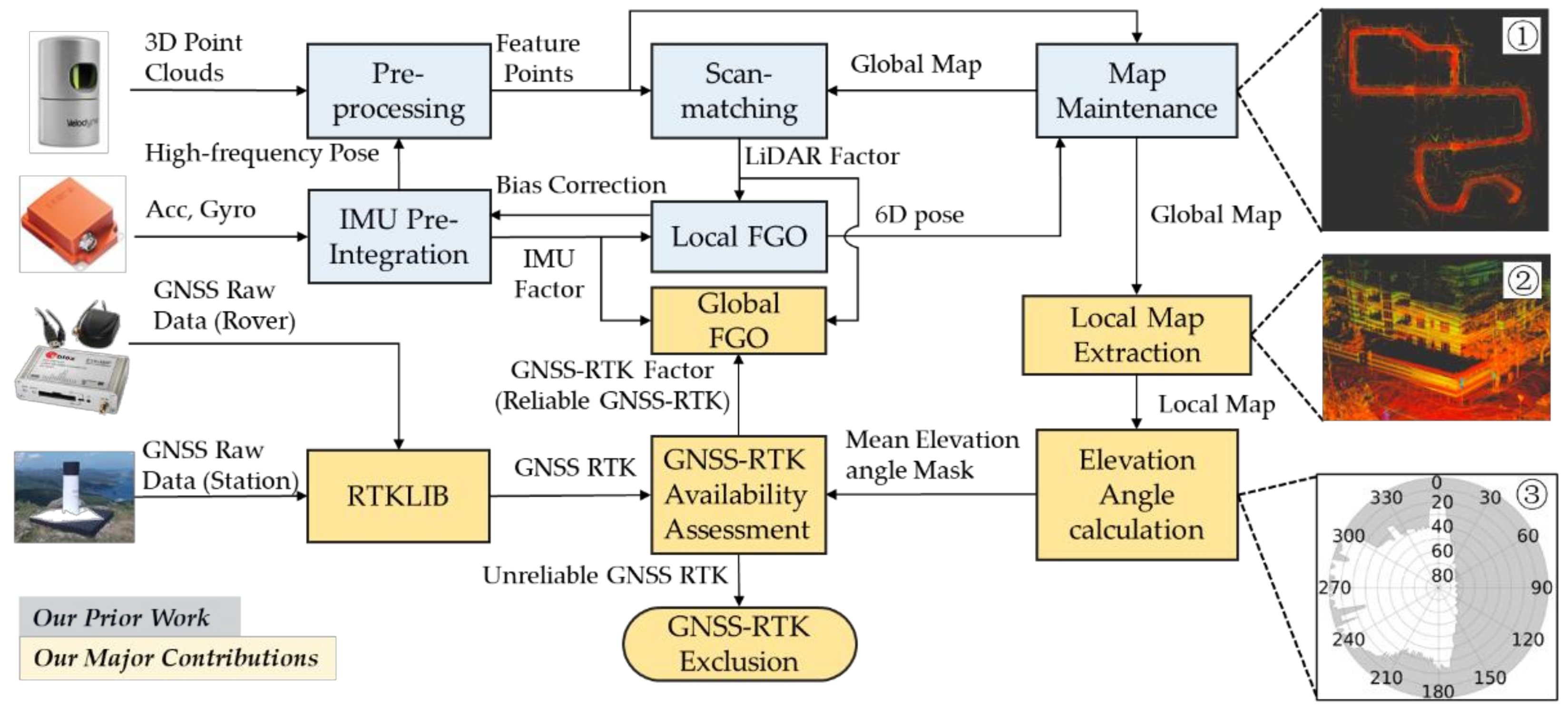
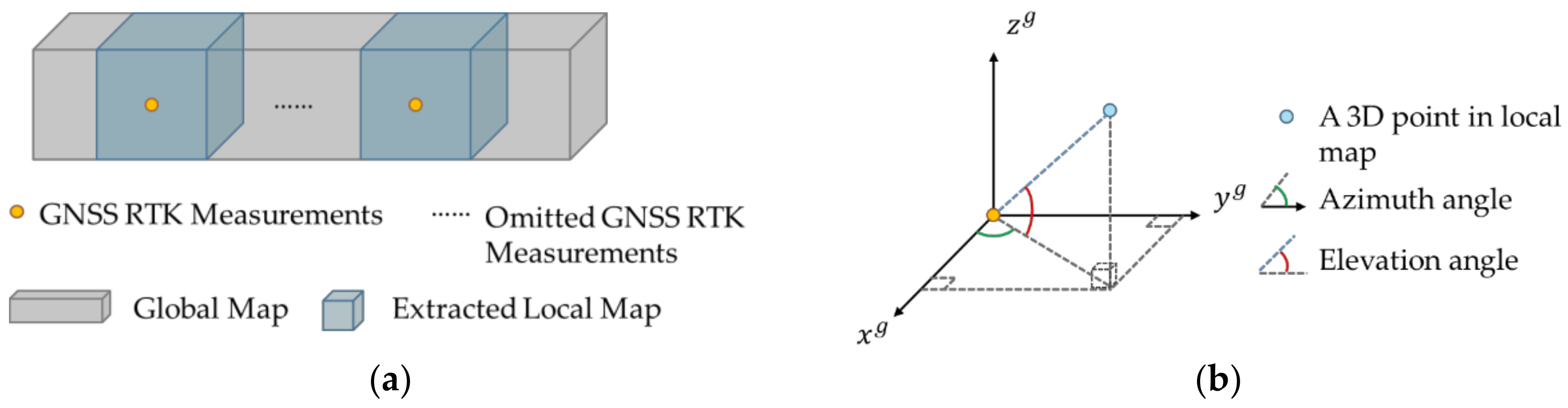
  • This paper proposed a GNSS-RTK availability assessment method, during which, unreliable GNSS measurements rejection is performed through mean elevation angle mask evaluation exploiting the registered 3D map that was incrementally constructed by LIO based on our previous work in [33]. It is worth mentioning that the mean elevation angle in this paper is defined as that generated by the buildings around the GNSS receiver rather than the satellites.
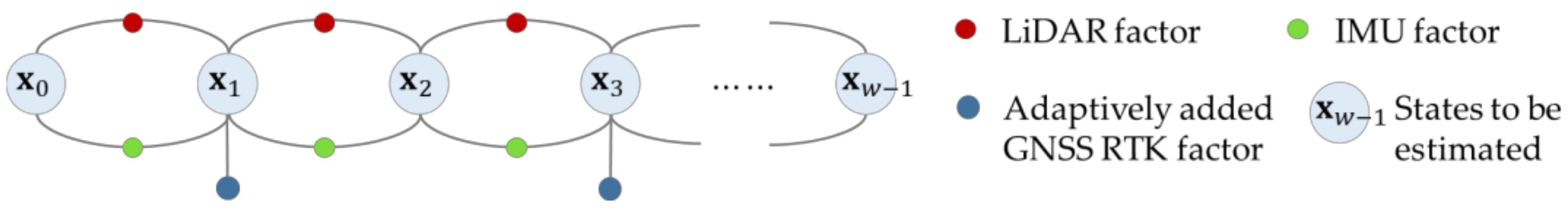
  • This paper proposed a GNSS-RTK/LIO integration scheme based on factor graph optimization. Concretely, the globally referenced positioning from reliable GNSS-RTK and relative pose estimation are integrated using the FGO [24] which is free of abnormal GNSS-RTK solutions.
  • The effectiveness of the proposed GNSS-RTK availability assessment and the adaptive sensor fusion is validated on three typical urban canyons datasets collected in Hong Kong [9].
The rest of the paper is structured as followed: In Section 2 materials and methods are presented. Concretely, an overview of the framework with pre-definitions of important mathematical symbols is introduced in Section 2.1. The GNSS-RTK availability assessment method which is the so-called GNSS-RTK selection procedure is described in Section 2.2. The adaptive sensor fusion method would be discussed in detail in Section 2.3. What is more, the experimental results are displayed in Section 3, along with discussions in Section 4. Conclusions and prospects are given in Section 5.

2. Materials and Methods

2.1. Overview of the Proposed Framework

The overview of the proposed framework is depicted in Figure 1. The boxes painted in blue are inherited from our previous work LC-LIO in [33] where we developed a factor graph-based LIO scheme. The yellow ones represent the main contributions in this paper. As receiving the 3D point clouds and the IMU ego-motion measurements, the LiDAR factor and IMU factor are constructed via scan-matching [43] and IMU pre-integration [44] respectively, and then jointly optimized in the sliding window based local FGO. A globally consistent map consisting of registered 3D points is incrementally generated with each local optimization accomplished. For more details about the LIO adopted in this paper, the full paper [33] is recommended. The GNSS raw data produced by the rover and station are firstly processed by RTKLIB [7] to obtain GNSS-RTK solutions. For each of the epochs, the surrounding local map is extracted from the global map. The mean elevation angle mask could be calculated according to the 3D point cloud map, after which GNSS-RTK availability is assessed. Given a predefined threshold, those with heavy mean elevation angle masks, indicating encirclement by skyscrapers, towering trees, etc., are supposed to be unreliable and excluded. Others with small mean elevation angle masks are in relatively open areas and are assumed to be reliable. A global FGO is executed for the fusion of LiDAR factor, IMU factor and GNSS-RTK factor created by reliable GNSS-RTK. A continuous and accurate georeferenced position is finally achieved.
Before diving into the expanded introduction of the proposed method, the coordinates involved are clarified as follows:
  • The LiDAR frame ·   l : Originated at the geometric center of the LiDAR.
  • The IMU frame ·   b : Originated at the geometric center of the IMU.
  • The GNSS measurement frame ·   g : Originated at the GNSS measurement with the orientation of the axes consistent with that of the LiDAR frame.
  • The local world frame ·   w : Coincide with the initial LiDAR frame.
  • The east-north-up (ENU) frame ·   n : Originated at the initial vehicle position with the x-axis, y-axis, and z-axis pointing to the east, north, and up respectively.
In this paper, matrices are denoted in upper-case and bold letters. Vectors are denoted in lowercase and bold letters. Variable scalars are denoted as lower-case and italic letters. Poses under different frames could be transferred via multiplication rules defined in the 3D Special Euclidean group (SE(3)) [45]. Concretely, T   n w represents the transformation matrix from the local world frame to the ENU frame. Following the Equation (1), the i -th map points f   w i 3 under the world frame would be transformed to the ENU frame and denotes as f   n i :
f   n i = T   n w f   w i .

2.2. GNSS-RTK Availablity Assessment

In this section, the mean elevation angle mask generation and the accompanying GNSS-RTK availability assessment are presented.
The first step is the local map extraction. Each GNSS-RTK resolved by RTKLIB [7] under the Earth-centered, Earth-fixed (ECEF) coordinate system is converted to the ENU frame through GeographicLib [46]. As shown in Figure 2a, the local map around it is extracted from the global map. The map is originally expressed under the local world frame and then converted to the ENU frame for convenience. What is more, in the “east” and “north” directions, the local map is specified by fixed Euclidean distance parameters. While in the “up” direction, all the points are included to completely reflect the density and the altitude of the obstacles. For computational efficiency, points lower than 1 m in the local map are removed.
The second step is a sub-region division which takes the evenness and the robustness into consideration. A total of 360 degrees around the GNSS rover is divided into 36 subregions according to the azimuth angle, for example, the point with an azimuth angle of smaller than 10 degrees belongs to the first subregion, and that bigger than 10 degrees but smaller than 20 degrees belongs to the second subregion. It is worth mentioning that the reliability of the GNSS measurements is not yet clear until the assessment is finished. Therefore, the chronologically closest pose estimated by local FGO is exploited instead of quantifying the relative distance between the GNSS rover and the scanned objects. Regarding the k -th GNSS-RTK solution g   n k = x   n g k   ,   y   n g k   ,   z   n g k   T , its correspondent position generated by local FGO is denoted as g ˜   n k = x   n g ˜ k   ,   y   n g ˜ k   ,   z   n g ˜ k   T . For a point f   n i = x   n f i   ,   y   n f i   ,   z   n f i   T on the extracted local map, its azimuth angle is denoted as a z f i is calculated as:
a z f i = a r c t a n ( y   n g ˜ k   y   n f i   / x   n g ˜ k   x   n f i   ) .
Its elevation angle e l f i is defined as:
e l f i = a r c t a n z   n g ˜ k   z   n f i   / x   n g ˜ k   x   n f i   2 + y   n g ˜ k   y   n f i   2 .
Considering all the points in one subregion, their elevation angles are sorted among which the upper quartile is taken as the elevation angle of this subregion. Then the mean elevation angle of all the subregions denoted as e l g k , is taken as the mean elevation angle mask of the GNSS RTK measurement g k n . Provided a threshold e l t h , the GNSS-RTK availability assessment is finally achieved by:
g   n k : e l g k > e l t h , unreliable e l g k < e l t h , reliable .
The effect of different thresholds is evaluated and discussed in the section of the experiment result.

2.3. Adaptive GNSS-RTK/LIO Fusion

The sensor fusion framework is constructed to estimate the motion states of the sensor carrier. Methods for such state estimation problems are extensively investigated which could be categorized as filter-based and non-linear optimization-based [45]. The filter-based method is typically a predictor and corrector architecture subjecting to the first-order Markov hypothesis [47]. The current state to be estimated is first predicted based on the last state and then corrected according to the motion model and the measurement model respectively [48].
The non-linear optimization-based method is typically a non-linear least-square problem. Concretely, the state estimation problem could be formulated as a Maximum A Posteriori (MAP) problem and then be converted to a Maximum likelihood Estimation (MLE) via Bayes’ Theorem [49,50]. With the assumption of the Gaussian noise model, through negative logarithmic transformation, it is finally expressed as a nonlinear least-squares problem [24]. Each known measurement, based on which the state estimation is performed, could be expressed as a function of the states to be estimated. The least-squares term, commonly called a residual term, is the Mahalanobis distance between the known measurements and its approximation derived from the states. The residuals are expected to be small and thus provide constraints to the states. The objective function during the non-linear optimization is the sum of all the residuals. A group of states that minimizes the objective function is considered as the best solution for the estimator [24]. As shown in our recent work [41], compared with the filter-based estimator such as EKF, the non-linear optimization-based ones can better employ the correlation between consecutive epochs of measurements simultaneously. Furthermore, the computational efficiency of non-linear optimization-based methods is enhanced by the sliding-window manner [51] which involves states over some time rather than all the states during an optimization.
The non-linear optimization-based state estimation framework could be interpreted as a factor graph, namely FGO. States to be estimated are denoted as vertexes. Residuals constraining the states are expressed as edges and called factors in the graph. The FGO aims at finding a group of states that conform to all edges best [24].
The factor graph of the adaptive GNSS-RTK/LIO fusion procedure, that is the global FGO module in Figure 2, is displayed in Figure 3. The states to be estimated in one window is the 6D pose at the frequency of estimations from LIO represented as
X = x 0 ,   x 1 ,   x 2 , , x w 1 ,  
x k = R   n k p   n k 0 1 SE 3 , k = 0 , , w 1 ,  
where w is the window size, R   n k Special Orthogonal Group (SO(3)) [45] is the relative rotation and p   n k 3 is the absolute translation. The R   n k could be expressed in Lie algebra [52] for derivation calculation as:
R   n k = exp φ k
φ k 3 is the correspondent Lie algebra of R   n k . · is the skew-symmetric matrix of φ k . exp · represents the exponential transformation namely Rodrigues’s Formula [53] between the two patterns.
The LiDAR factor constructed from scan-matching provides relative motion constraints. The motion increment derived from scan-matching is taken as the known measurements functioning as a reference, while that computed via states to be estimated are considered as observed measurements. The factor is designed to minimize the difference between them as follows:
r L , k T   n l k 1 , T   n l k , X = T   n l k 1 1 · T   n l k 1 x k 1 1 · x k ,
in which T   n l k are solved by scan-matching.
The IMU factor derived from pre-integration is formulated in a similar way. The motion increment provided by IMU pre-integration and that derived from the states to be estimated are considered known measurements and observed measurements respectively. The difference between them namely the IMU factor is defined as below:
r B , k Z   n b k b k 1 , X = Z   n b k b k 1 1 x k 1 1 · x k ,
in which Z   n b k b k 1 SE 3 is the rotation and translation increment pre-integrated by IMU raw data with the bias corrected by local FGO. It is converted from the IMU frame to the ENU frame.
The adaptively added GNSS factor once a GNSS-RTK solution is judged to be reliable by the GNSS-RTK availability assessment module directly restricts the position part of the state as follows:
r G , j g   n j , X = g   n j p   n j , j 0 , w ,
where g   n j is the known measurement of the position provided by GNSS-RTK. The difference between the position to be estimated and g   n j is expected to be small. When the commercial-level GNSS receiver is exploited to generate location measurements under urban canyons, only 2D residuals respectively at the “earth” and the “north” direction are fused in the global optimization make more sense given the large error at the “up” direction.
In short, the full objective function of the global optimization could be expressed as the sum of all the residuals in a window:
f X = k = 1 , , w 1 ρ r L , k T   n l k 1 , T   n l k , X C L , k 2              + k = 1 , , w 1 ρ r B , k Z   n b k b k 1 , X C B , k 2          + j 0 , w ρ r G , j g   n j , X C G , j 2 .
In which · Σ 2 = · T Σ 1 · is the Mahalanobis distance. ρ · is the Cauchy Kernel [54] for outlier suppression expressed as
ρ s = c 2 log 1 + s c 2 ,
The control parameter c is set to 1 in our implementation [51]. C L , k is the covariance matrix weighting the confidence of the factor and is supposed to be constant in our implementation. C B , k is the covariance matrix for the IMU factor and is iteratively derived during the pre-integration according to the covariance propagation rule used when a linear transformation is performed on a random variable [44]. C G , j is the covariance matrix for the adaptively added GNSS-RTK factor and is assumed to be constant due to no further information quantitatively indicating the quality of the solution is taken into account such as the Ambiguity Dilution of Precision (ADOP) and the Position Dilution of Precision (PDOP) [55], among which the ADOP is based on the determinant of the covariance matrix of the least-squares ambiguities and defined as follows [56]:
ADOP = d e t Q a ^ 1 n ( cycle )
where Q a ^ is the covariance matrix of the ambiguities and n is its order.
The estimated states could be derived as:
X = min X 1 2 f X .
Levenberg-Marquardt (L-M) algorithm [57] implemented in Ceres Solver [58] is utilized to solve the non-linear optimization problem during which the residuals are minimized. The states in a window are updated iteratively until convergence. As for the i -th iteration, the update procedure is as follows:
J T J + λ I Δ X i = J T r ,
X i + 1 = X i Δ X i ,
in which, λ is the damping factor of the L-M algorithm automatically set according to the reduction of the residuals to control the step of the states. “ ” denotes that for each state x k , i + 1 = x k , i Δ x k , i . r represents the residual of each factor shaping to a column vector as follows:
r = r L , 1 T , , r L , w 1 T , r B , 1 T , , r B , w 1 T , r G , j 1 T , , r G , j n T T
For brevity, the r L , · , r B , · , and r G , j n with j n 0 , w denotes the residual of the LiDAR factor, the IMU factor, and the adaptively added GNSS-RTK factor respectively. J is the jacobian matrix of r referring to X expressed as follows:
J = r X = r x 0 ,     r x 1 ,     , r x w 1 = r L , 1 x 0   r L , 1 x 1   r L , 1 x w 1   r L , w 1 x 0 r L , w 1 x 1 r L , w 1 x w 1 r B , 1 x 0 r B , 1 x 1 r B , 1 x w 1   r B , w 1 x 0 r B , w 1 x 1 r B , w 1 x w 1 r G , j 1 x 0 r G , j 1 x 1 r G , j 1 x w 1 r G , j n x 0   r G , j n x 1   r G , j n x w 1   ,
Fortunately, the residual of each factor is only related to one or two states rather than most of the states as shown in Figure 3 [59]. In other words, the matrix J and J T J are both sparse. Therefore, computational efficiency is guaranteed.

3. Results

3.1. Experimental Setup

Sensor setups: To validate the effectiveness of the proposed method, the experiment is conducted on three datasets collected in typical urban canyons in Hong Kong. As shown in Figure 4a,b, the Velodyne HDL-32E was employed to collect 3D point clouds at a frequency of 10 Hz. The Xsens Ti-10 IMU was employed to collect acceleration and angular velocity at a frequency of 200 Hz. A commercial-level u-blox GNSS receiver was used to collect the raw GNSS measurements, based on which the GNSS-RTK solution was further calculated by RTKLIB [7]. Besides, the NovAtel SPAN-CPT, a GNSS (GPS, GLONASS, and Beidou) RTK/INS (fiber-optic gyroscopes, FOG) integrated navigation system was used to provide the ground truth. In the SPAN-CPT, the high-end INS are integrated with GNSS to ensure continuous position estimation during GNSS outage. The NovAtel Inertial Explorer is also exploited to deliver precise positioning results. The ground truth provided by the SPAN is reliable and precise enough for evaluation. All the data were collected and synchronized using ROS [60]. The extrinsic parameters among all the sensors were calibrated in advance.
Table 1 summarizes the three datasets on which the framework proposed in this paper is verified, namely UrbanNav-HK-Data20190428, UrbanNav-HK-Deep-Urban-1, and UrbanNav-HK-Data20210714, abbreviated as urban-1, urban-2, and urban-3 respectively in the following. The first two data are contained in our recently open-sourced UrbanNav dataset [9]. As shown in Figure 5a, urban-1 is collected at Tsim Sha Tsui (an urban scenario with buildings and trees in Hong Kong) with a total length of 2.01 km. As shown in Figure 5b, urban-2 is collected at Whampoa (an urban scenario with dense buildings in Hong Kong) from which the last 2.37 km is selected for the experiment. As shown in Figure 5c, urban-3 is collected from Whampoa to Tsim Sha Tsui with a much longer length of 4.3 km.
The settings specified in the RTKLIB are listed in Table 2. The settings specified in the RTKLIB when processing the raw GNSS measurements from u-blox to achieve GNSS-RTK solutions for the three datasets are listed in Table 2 respectively.
Evaluation metrics: The validity of the GNSS-RTK availability assessment method and the adaptive GNSS-RTK/LIO fusion pipeline for positioning are investigated. The 3D absolute translation error (ATE) implemented in EVO [61] is defined as follows:
e k = p   n k , e s t p   n k , g t 2 ,
In which, p   n k , e s t 3 and p   n k , g t 3 represents the estimated position and the ground truth of the k -th epoch respectively. ·   2 denotes the 2-norm. e k is the ATE of p   n k , e s t . The quantitative comparison of the estimated position from different pipelines is performed by comparing the Root Mean Square Error (RMSE) of ATE to the total traveled length.
Evaluated methods: To verify the contributions of the proposed method in this paper, we evaluated the following methods.
  • Method1: This indicates the conventional GNSS/LIO fusion method [34,42,62] that directly integrates all the received GNSS-RTK measurements, among which LIO-SAM [42] is open-sourced. In the fusion method proposed in this paper, the threshold for GNSS availability would be set as 90 ° equivalently. To be more convincing, the performance of LIO-SAM [42] is also evaluated.
  • Method2: This indicates the adaptive GNSS/LIO fusion methods with a different threshold ( e l t h ) in Equation (4) for the GNSS-RTK solution selection proposed in this paper. For urban-1, the threshold is selected as 35 ° and 15 ° . For urban-2 and urban-3, besides these two thresholds, 20 ° is additionally selected for a sufficient evaluation.
Besides the above-mentioned positioning results of the various integrated pipelines, the positioning accuracy of alone GNSS-RTK measurements and LIO are also shown for exhaustive performance analysis. It is worth mentioning that the LIO here represents the loosely coupled LiDAR-inertial fusion method implemented in our previous work [33] which is different from that in the tightly coupled framework LIO-SAM [42].

3.2. Experimental Results in Urban Canyon 1

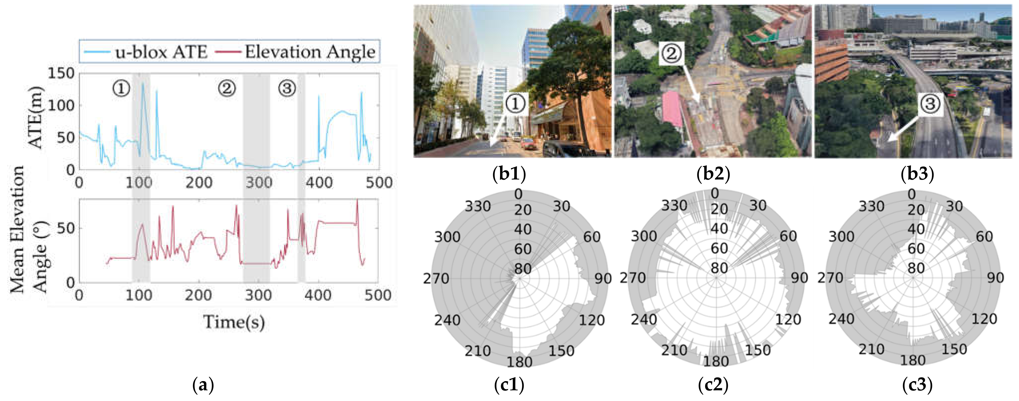
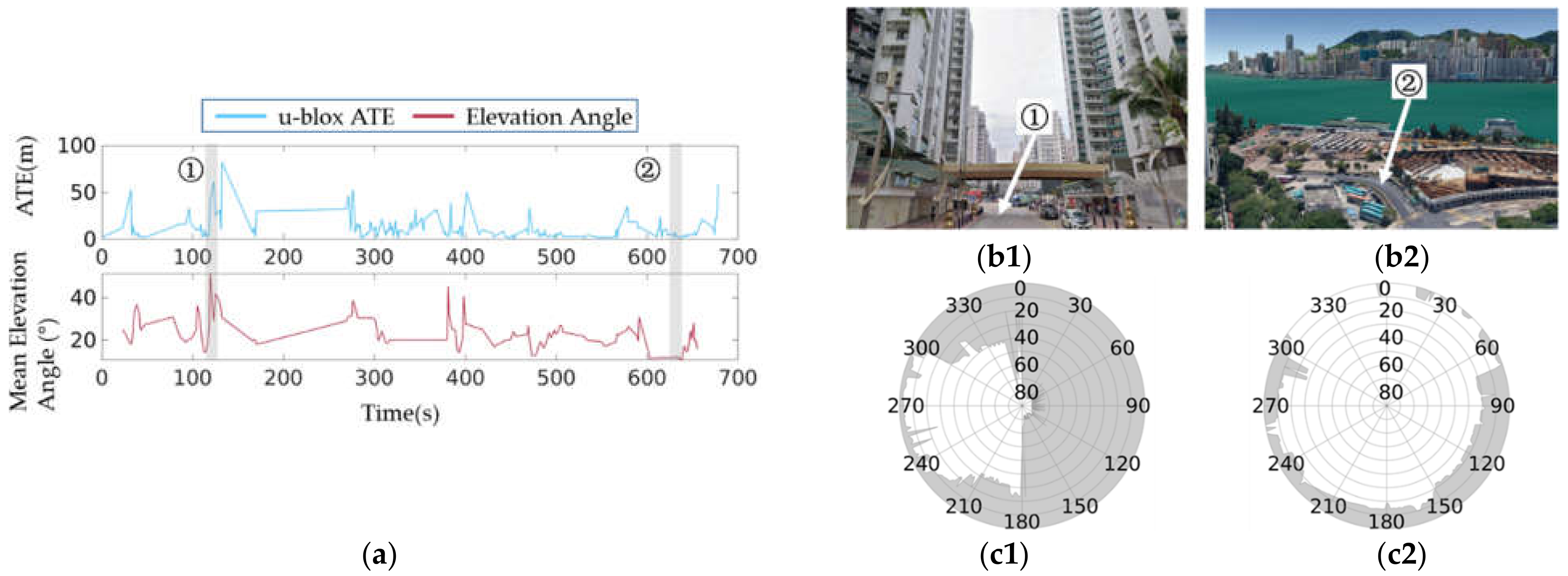
3.2.1. Results of GNSS-RTK Availability Assessment

To evaluate the proposed GNSS-RTK availability assessment method, the ATE of the u-blox measurement and the corresponding mean elevation angle mask of the surrounding local map is depicted in Figure 6a with three representative places annotated. The mean elevation angle mask is defined as that of a fixed-size local map with 50 m (Euclidean distance) both forward and backward of the rover. Thus, u-blox epochs within 50 m from the start and the end have no corresponding mean elevation angle masks. Figure 6b displays streetscapes in these three places. Figure 6c shows the elevation angle mask at each subregion of the local point cloud map 360 degrees around the place. It is worth mentioning that the direction from 0 ° to 360 ° on the outermost circle, namely the azimuth angle defined by Equation (2), refers to the position of the 3D LiDAR sensor, thus depending on the scanning pattern of the LiDAR at the correspondent epoch. As for Velodyne HDL-32E, the 0 ° direction at different epochs changes continuously for all-around detection. It is not equal to the forward direction of the vehicle. For consistency, the directions on each elevation angle mask are labeled clockwise with the 0 ° direction upward. The elevation angles ( ° ) are depicted by concentric circles increasing from the outside to the inside.
The ① place has skyscrapers almost on three sides with more than half part of the sky mask reaching up to 50 ° shown in Figure 6b1,c1, respectively. As displayed in Figure 6a, the calculated mean elevation angle mask and the ATE of the u-blox are consequently large, which implies the GNSS-RTK solution is unavailable. What is more, at the ② place as shown in Figure 6b2, there is an open crossroad. Consistent with the scenario, the estimated mean elevation angle mask illustrated in the bottom panel of Figure 6a,c2, and the ATE of the u-blox illustrated in the top panel of Figure 6a, are notably small meaning that the GNSS-RTK solution tends to be reliable. However, at the ③ place shown in Figure 6b3, it is open near Victoria Harbor. The u-blox measurement is significantly accurate, seen in the top panel of Figure 6a. Unexpectedly, the elevation angle mask is large, with more than one-third reaching up to 40 ° , as shown in Figure 6c3, due to the tall trees detected in the point cloud map.

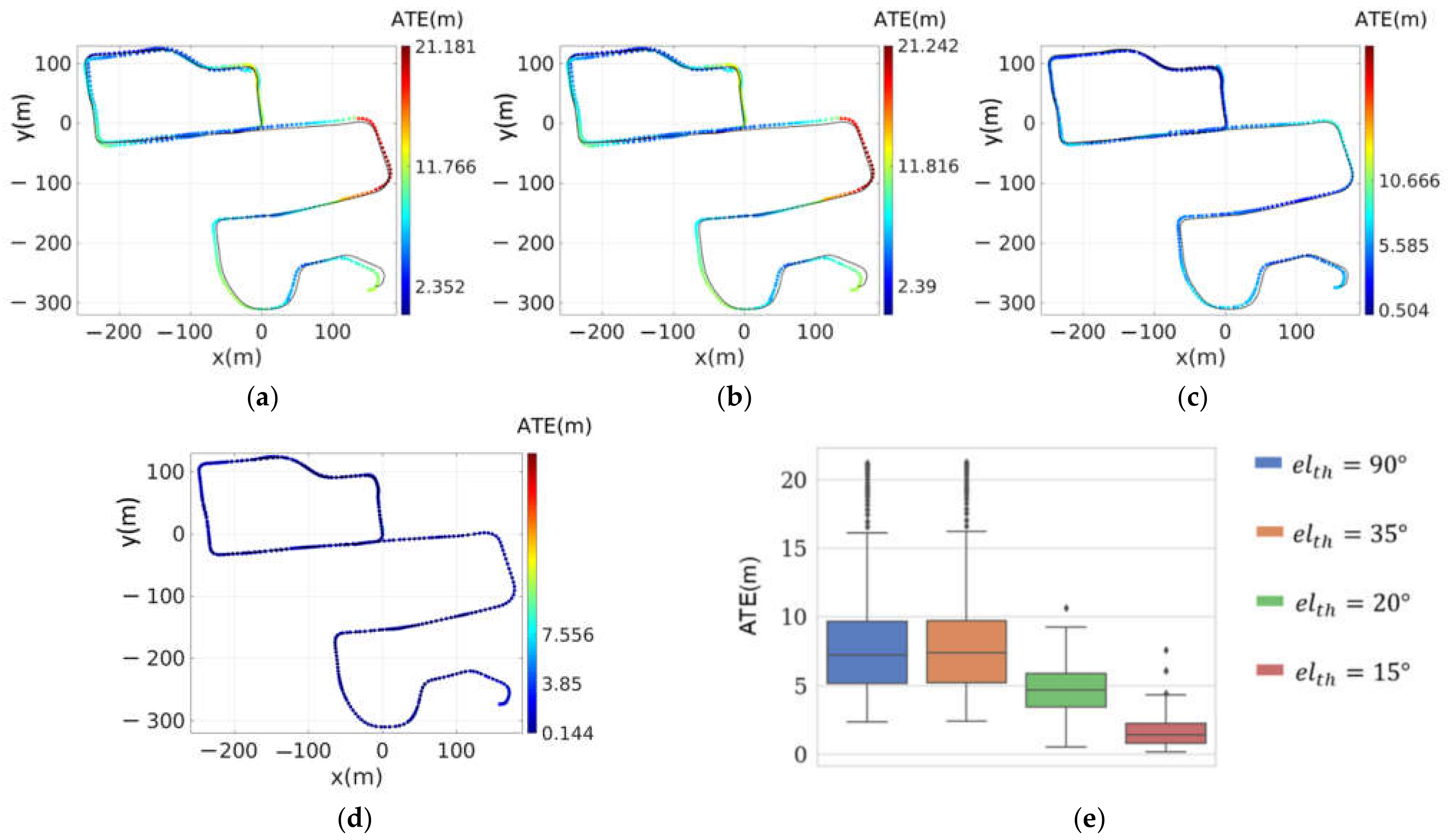
3.2.2. Positioning Results Comparison

To validate the effectiveness of the adaptive GNSS-RTK/LIO fusion method for continuous position estimation, the trajectories generated by the adaptive integrated pipelines with thresholds e l t h for the GNSS-RTK availability assessment equals 90 ° , 35 ° , and 15 ° are presented respectively in Figure 7a–c. All the u-blox RTK solutions processed by RTKLIB [7], among which no fixed ones were reported, with a mean elevation angle mask smaller than e l t h are fused with LiDAR and IMU measurements as Equation (11). When e l t h equals 90 ° , as the mean elevation angle mask must be smaller than 90 ° , all the developed u-blox RTK solutions are integrated. Unavailable solutions with large errors would destroy the estimation, while the smaller e l t h rejects more unavailable ones, and therefore make more accurate position estimation. As shown in Figure 7a–c, the smaller e l t h is, the better its corresponding trajectory overlaps with the ground truth. The box plot in Figure 7d further shows the precision of the three trajectories quantitatively.
Table 3 shows the precision of the positioning results from alone GNSS-RTK measurements, the LIO, the LIO-SAM [42], and the three adaptive integrated pipelines quantitatively. The ATE of the pure GNSS-RTK is quite large with an RMSE of 42.02 m. The LIO achieves the best precision with the RMSE of 3.99 m as marked in bold font. The RMSE of ATE of the position estimated by the traditional fusion method LIO-SAM [42] is about 19.89 m. Among the adaptive integrated GNSS-RTK/LIO methods, when e l t h equals 90 ° , the RMSE of ATE is 25.33 m. In LIO-SAM [42], only when the covariance of the pose generated by LIO exceeds a preset threshold, which means the reliability of the LIO decreases, the GNSS-RTK solutions without assessment are included for state optimization and correction. The proposed fusion pipeline with e l t h equals 90 ° fused all the received GNSS-RTK solutions which would be more than that used in LIO-SAM [42]. Considering that the GNSS-RTK solution on this data has a large error, the positioning accuracy of the proposed pipeline with e l t h equals 90 ° is lower than that of LIO-SAM [42] consequently. By decreasing the e l t h to 35 ° , a 25% improved RMSE of 18.88 m is achieved. With e l t h set to 15° the next best precision is obtained.

3.3. Experimental Results in Urban Canyon 2

3.3.1. Results of GNSS-RTK Availability Assessment

To challenge the performance of the proposed method, the other dataset is further evaluated on a denser urban scenario, the urban-2. The ATE of the u-blox measurement and the correspondent mean elevation angle mask of the surrounding local map is depicted in Figure 8a. A similar trend can also be seen in that large mean elevation angle masks are accompanied by u-blox solutions with large ATE and vice versa. In detail, at the ① place seen in Figure 8b1, the footbridge in the front of the vehicle and skyscrapers on both sides result in poor GNSS solutions with large ATE. More than half of the corresponding sky mask of the surrounding point cloud reaches up to 60 ° calculated as the Equation (3) shown in Figure 8c1. Then, the ② place, displayed in Figure 8b2, is open near the bay which leads to accurate GNSS solutions with small ATE. Conforming to the scene, most elevation angles depicted in the mask in Figure 8c2 are smaller than 30 ° .

3.3.2. Positioning Results Comparison

The effectiveness of the adaptive GNSS-RTK/LIO fusion method for continuous position estimation is further validated on urban-2. The trajectories generated by the adaptive integrated pipelines with thresholds e l t h for the GNSS-RTK availability assessment equals 90°, 35°, 20°, and 15° are presented respectively in Figure 9a–d. Different from urban-1, fixed u-blox RTK solutions processed by RTKLIB [2] are reported on urban-2. Among the fixed ones, the corresponding mean elevation angle mask of which is smaller than e l t h , are fused with LiDAR and IMU measurements as Equation (11) in our experiments. It is noteworthy that when fixed solutions are developed, the surroundings are relatively empty. The mean elevation angle mask of such places would be relatively small. Specifically, on urban-2 only one fixed solution has a mean elevation angle mask larger than 35°. Therefore, trajectories estimated by pipelines with e l t h set to 90° and 35° achieves similar accuracy as plotted in Figure 9a,b. As e l t h decreasing, the percentage of available GNSS RTK solutions to integrate with LiDAR and IMU measurements increases. As a consequence, the estimated trajectory achieves better accuracy. As shown in Figure 9c,d, the estimated trajectories are in better agreement with the ground truth. The box plot in Figure 9d compares the precision of the four trajectories quantitatively.
Table 4 shows the precision of the positioning results from alone GNSS-RTK measurements, the LIO, and the four adaptive integrated pipelines quantitatively. Overall speaking, the positioning results on urban-2 are more accurate compared to that on urban-1 thanks to fixed solutions. The ATE of the pure GNSS-RTK is still large with an RMSE of 15.75 m. The LIO achieves the next best precision with the RMSE of 1.80 m. The RMSE of ATE of the position estimated by LIO-SAM is improved compared with GNSS RTK alone but still large due to the reliability of the fused GNSS RTK solutions is not proved. Among the four adaptive integrated pipelines, when e l t h equals 90 ° and 35 ° , comparable positioning precision is achieved. The RMSE of ATE is about 8.6 m. By decreasing the e l t h to 20 ° , the RMSE is significantly improved by 50% to 4.86 m. The pipeline with e l t h set to 15° achieves the best precision with the RMSE of 1.738 m as marked in bold font in Table 2.

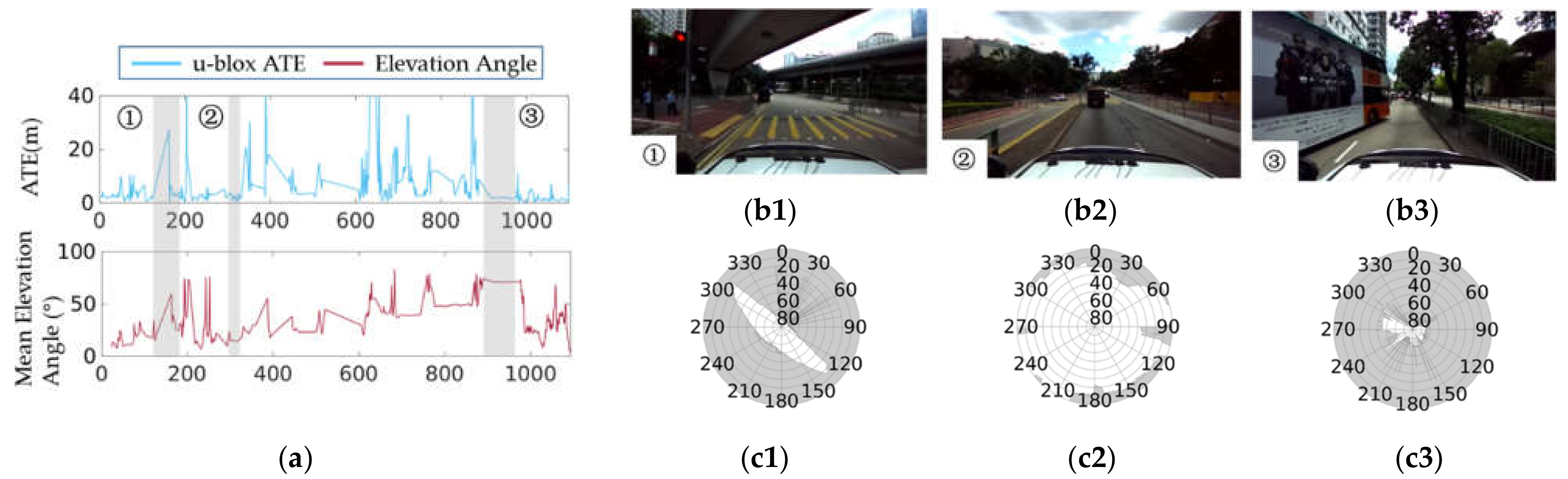
3.4. Experimental Results in Urban Canyon 3

3.4.1. Results of GNSS-RTK Availability Assessment

To perform extensive validation of the proposed method, the experiment is implemented on the urban-3 with a much longer length. The ATE of the u-blox measurement and the correspondent mean elevation angle mask of the surrounding local map is depicted in Figure 10a. The mean elevation angle masks and the ATE of the u-blox solutions are roughly correlated. When the ATE of the u-blox solution becomes large, the corresponding mean elevation angle mask would become large following and vice versa. In detail, at the ① place seen in Figure 10b1, the overpasses over the vehicle result in poor GNSS solutions with large ATE. More than half of the corresponding sky mask of the surrounding point cloud reaches up to 60 ° calculated as the Equation (3) shown in Figure 10c1. Then the ② place, displayed in Figure 10b2, is relatively open with low objects on both sides which leads to accurate GNSS solutions with small ATE. Conforming to the scene, most elevation angles depicted in the mask in Figure 10c2 are smaller than 30 ° . Around the ➂ place, which is near an open crossing, the ATE of the u-blox solutions is small due to the unblocked transmission of the signal as shown in the top panel of Figure 10a. However, the mean elevation angle mask calculated from the point cloud is particularly large as shown in the bottom panel of Figure 10a. The false evaluation is caused by the trees over the vehicle and the tall double-decker bus around detected by the LiDAR presented in Figure 10b3. Most elevation angles of the surrounding points are larger than 60 degrees as plotted in the sky mask in Figure 10c3.

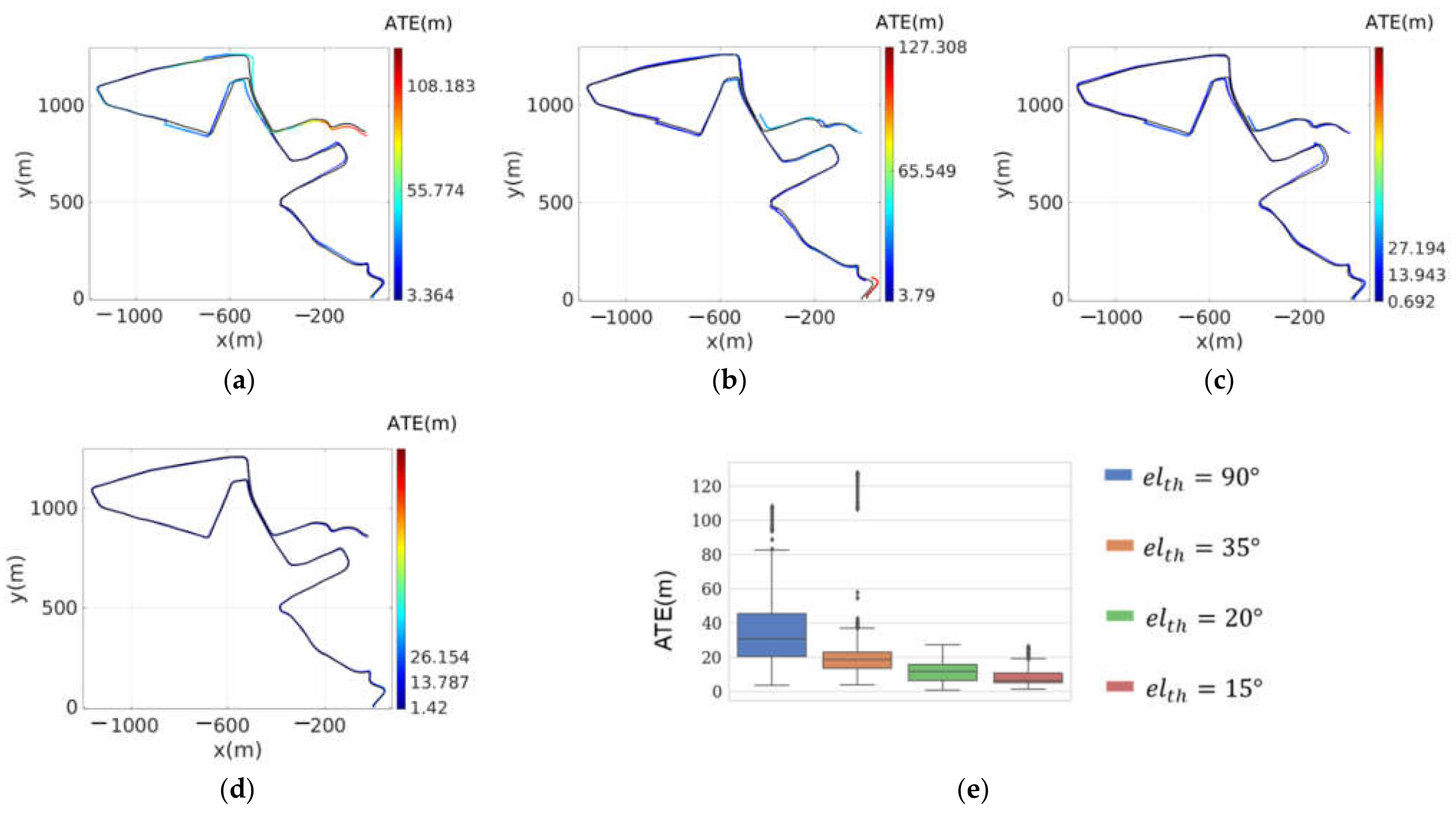
3.4.2. Positioning Results Comparison

The effectiveness of the adaptive GNSS-RTK/LIO fusion method for continuous position estimation is validated on urban-3. The trajectories generated by the adaptive integrated pipelines with thresholds e l t h for the GNSS-RTK availability assessment equals 90°, 35°, 25°, and 15° are presented respectively in Figure 11a–d. Fixed u-blox RTK solutions processed by RTKLIB [2] are reported on urban-3 as on urban-2. Among the fixed ones, the corresponding mean elevation angle mask of which is smaller than e l t h , are fused with LiDAR and IMU measurements as Equation (11) in our experiments. As e l t h decreasing, the estimated trajectory achieves better accuracy which would be in better agreement with the ground truth. The box plot in Figure 11d compares the precision of the four trajectories produced by the adaptive fusion pipelines quantitatively.
Table 5 shows the precision of the positioning results from alone GNSS-RTK measurements, the LIO, the LIO-SAM [42], and the four adaptive integrated pipelines quantitatively. Overall speaking, the ATE of the positioning results on urban-3 are large. The RMSE of ATE of the pure GNSS-RTK reaches up to 22.23 m. The LIO achieves the next best precision with the RMSE of 11.43 m suffering from accumulated drift. Among the four adaptive integrated pipelines, when e l t h varies from 90 ° to 15 ° , the RMSE of ATE is gradually improved. The precision of the LIO-SAM is comparable with the proposed method with e l t h equal 90 ° , both of which are categorized as conventional fusion methods. The pipeline with e l t h set to 15° achieves the best precision with the RMSE of 10.02 m as marked in bold font in Table 3.

4. Discussion

4.1. Performance of GNSS-RTK Availability Assessment

The GNSS-RTK Availability Assessment method proposed in the paper functions as selecting available GNSS-RTK solutions under urban canyons for further fusion with LIO. The exclusion of unavailable GNSS-RTK solutions with potential large errors guarantees the convergence and the accuracy of the optimization-based fusion. The availability assessment is implemented by evaluating the mean elevation angle mask of the buildings surrounding the GNSS-RTK solution as Equation (3). It benefits from the 3D range information perceived by LiDAR and the accurate point cloud map produced by LiDAR/inertial odometry. A large mean elevation angle mask indicates tall objects around. While a small one indicates open areas.
Ideally, under urban scenarios, a large mean elevation angle mask implies deep urban canyons and thus the ATE of the GNSS-RTK measurements should be large due to signal blockage or reflection. Such as the three places denoted as “➀” in Figure 6, Figure 8 and Figure 10. Oppositely, a small mean elevation angle mask denotes unblocked areas and the ATE of the GNSS-RTK measurements is expected to be small. Such as the three places denoted as “➁” in Figure 6, Figure 8 and Figure 10. Most cases shown in the experiments on the three datasets are in line with the above law. Hence, available GNSS-RTK solutions could be selected according to the mean elevation angle mask. The correctness of the GNSS-RTK availability assessment via calculating the mean elevation angle mask of the point cloud map is validated.
However, false GNSS-RTK availability assessment under relatively open areas would occur affected by tall and dense trees, etc. Such as the two places denoted as “➂” in Figure 6 and Figure 10. These trees detected by the LiDAR over the vehicle would derive a large mean elevation angle mask while their influence on GNSS positioning accuracy is not that great. Such false assessment would miss really available GNSS-RTK solutions occasionally. To avoid this, semantic annotation of the 3D point map would be conducive to eliminate the influence of the tall objects nearby which will be one of our future works.

4.2. Performance of Adaptive GNSS-RTK/LIO Fusion

  • The continuous and smooth GNSS-RTK positioning under urban canyons with LIO.
Under deep urban canyons, the positioning results of the GNSS-RTK are likely to be discontinuous between epochs due to poor signal transmission [63]. The ATE of the GNSS-RTK measurements is consequently large, as shown in the first row of Table 1, Table 2 and Table 3. With the assistance of LIO, the positioning accuracy of the integrated pipelines is improved by more than 50% compared with that of the GNSS-RTK alone as shown in the last three rows of Table 3 and the last four rows of Table 4 and Table 5. What is more, the visualized trajectory is smooth and continuous as shown in Figure 7c, Figure 9d and Figure 11d. In conclusion, through integration with LIO, the continuous and smooth positioning of GNSS-RTK under deep urban canyons is realized.
  • The accumulated drift alleviation of LIO with GNSS-RTK.
As local sensors, LiDAR and IMU could only provide relative motion estimations. Therefore, accumulated drift is unavoidable. Theoretically, in the fusion with the absolute positioning solutions from GNSS-RTK, the drift would be corrected. However, in our experiments on the three typical urban scenarios, the original GNSS-RTK solutions provided by the commercial level receivers are notably poor with tens of meters error as shown in the first row of Table 3, Table 4 and Table 5. For urban-1, no fixed GNSS-RTK solutions are provided. The RMSE of the ATE of the LIO is even slightly better than the best adaptive fusion positioning results, as shown in the second row and the last row of Table 3. On urban-2 and urban-3, with more fixed GNSS-RTK solutions developed, the RMSE of the ATE of the best adaptive fusion positioning results are better compared with that of LIO. The accumulated drift of LIO would be more alleviated as the quality of the GNSS-RTK measurements is improved. GNSS measurements refinement after selection would be a promising strategy for a further breakthrough.
  • The superiority of the proposed adaptive GNSS-RTK/LIO integration.
The proposed adaptive GNSS-RTK/LIO integration pipeline periodically performs a non-linear optimization-based fusion of GNSS-RTK and LIO, once the GNSS-RTK solution is assessed as available by the GNSS-RTK availability assessment module. As shown in the last three rows of Table 3 and the last four rows of Table 4 and Table 5, the best precision achieved with the adaptive fusion pipeline is improved by more than 75% compared with that of the traditional method. The superiority of the proposed method is validated.
By lowering the threshold for the assessment, more unavailable GNSS-RTK solutions would be rejected. The ATE of the positioning results is continuously improved. Moreover, the visualized trajectories are smoother as plotted in Figure 7a–c, Figure 9a–d and Figure 11a–d. The effectiveness of the GNSS-RTK availability assessment is further demonstrated. Theoretically, the pipeline with the smallest threshold always achieves the best precision. However, in our experiments in the deep urban canyons with dense skyscrapers, when the threshold is smaller than 15° there is hardly any GNSS RTK solutions could be selected as available. In other words, 15° is the best threshold for the proposed method tested on deep urban canyons such as our UrbanNav dataset. When running on less urban dataset, the best threshold for the proposed method would be lower than 15°.
Nevertheless, the best precision achieved by the adaptive fusion method is still at meter-level due to the poor GNSS measurements provided by commercial level receivers in urban canyons. Deeper sensor fusion to correct the GNSS measurement model would lead to enhancement.

5. Conclusions and Prospects

This paper proposes a GNSS-RTK availability assessment method exploiting the registered 3D point map provided by LiDAR. Further integration of the available GNSS solutions, LiDAR, and IMU measurements are implemented, namely adaptive sensor fusion pipeline, to perform absolute position estimation under deep urban for autonomous navigation. The effectiveness of the GNSS-RTK availability assessment via mean elevation angle mask calculation of the local point cloud map is firstly verified according to the ATE of the GNSS measurements. For example, in most cases, a large mean elevation angle mask could be achieved under a sheltered environment. The GNSS would be assumed to be unavailable. Correspondingly, the ATE of the GNSS measurements tends to increase. With the help of the proposed GNSS-RTK selection method, poor GNSS solutions with large errors are excluded before the fused positioning. The trajectories estimated by such an adaptive fusion scheme are investigated quantitatively and qualitatively. During the experiments, different percentages of available GNSS solutions are leveraged as the threshold for availability assessment is tuned. The precision of the estimated trajectory is gradually improved as the percentage increases. In summary, the capabilities of the GNSS-RTK availability assessment module to avoid unavailable GNSS solutions and the adaptive fusion method to continuously estimate the position are demonstrated. However, the proposed method can be significantly challenged when the long-term GNSS interruption occurs. Specifically, the locally generated map will not be reliable for the GNSS-RTK selection due to the accumulated drift from the LiADR/inertial odometry. Integrating more sensors to mitigate the potential drift of the LiADR/inertial odometry will be one of the possible future research directions.
For future studies, we would further improve the accuracy of the position estimation from meter levels to centimeter levels. The semantic map [64,65,66] with labeled objects would contribute to avoiding false GNSS unavailability assessment under open areas. Because the tall trees and other nearby objects which lead to large mean elevation angle masks could be noted and removed. Moreover, it can be seen from the integrated positioning results on the three urban canyons, that the achieved best positioning precisions are still meter levels. This is because all the GNSS-RTK solutions provided by the commercial level GNSS receiver are inaccurate due to the dense building structures. Therefore, GNSS solutions refinement via measurement model correction during deeper sensor fusion would be promising [67,68]. Last but not least, the extrinsic parameters among different sensors make great sense [69]. Online calibration and adjustment are expected to be helpful [70,71].

Author Contributions

Conceptualization, Y.W., L.-T.H., W.W. and J.Z.; methodology, W.W. and J.Z.; software, J.Z. and F.H.; validation, J.Z.; investigation, W.W. and J.Z.; resources, Y.W. and L.-T.H.; data curation, W.W., F.H. and J.Z.; writing—original draft preparation, J.Z.; writing—review and editing, W.W., L.-T.H. and J.Z.; supervision, L.-T.H. and X.C. All authors have read and agreed to the published version of the manuscript.

Funding

This research was funded by Riemann Laboratory, Huawei Technologies grant number ZGD2. The APC was also funded by Riemann Laboratory, Huawei Technologies. This research was also supported by the Faculty of Engineering, The Hong Kong Polytechnic University under the project “Perception-based GNSS PPP-RTK/LVINS integrated navigation system for unmanned autonomous systems operating in urban canyons”. This research was also supported by the Guangdong Natural Science Foundation (2021A1515110771).

Acknowledgments

We would like to thank our colleague Hoi-Fung Ng for his kind help with the visualization of the mean elevation angel mask for GNSS-RTK solutions.

Conflicts of Interest

The authors declare no conflict of interest.

References

  1. Alatise, M.B.; Hancke, G.P. A review on challenges of autonomous mobile robot and sensor fusion methods. IEEE Access 2020, 8, 39830–39846. [Google Scholar] [CrossRef]
  2. Zhang, J.; Khoshelham, K.; Khodabandeh, A. Seamless Vehicle Positioning by Lidar-GNSS Integration: Standalone and Multi-Epoch Scenarios. Remote Sens. 2021, 13, 4525. [Google Scholar] [CrossRef]
  3. Wen, W.; Zhou, Y.; Zhang, G.; Fahandezh-Saadi, S.; Bai, X.; Zhan, W.; Tomizuka, M.; Hsu, L.-T. Urbanloco: A full sensor suite dataset for mapping and localization in urban scenes. In Proceedings of the 2020 IEEE International Conference on Robotics and Automation (ICRA), Paris, France, 31 August–31 May 2020; pp. 2310–2316. [Google Scholar]
  4. Chen, Y.; Tang, J.; Jiang, C.; Zhu, L.; Lehtomäki, M.; Kaartinen, H.; Kaijaluoto, R.; Wang, Y.; Hyyppä, J.; Hyyppä, H.; et al. The accuracy comparison of three simultaneous localization and mapping (SLAM)-based indoor mapping technologies. Sensors 2018, 18, 3228. [Google Scholar] [CrossRef] [PubMed] [Green Version]
  5. Kaplan, E.D.; Hegarty, C. Understanding GPS/GNSS: Principles and Applications; Artech House: London, UK, 2017. [Google Scholar]
  6. Wen, W.; Hsu, L.-T. Towards Robust GNSS Positioning and Real-time Kinematic Using Factor Graph Optimization. In Proceedings of the 2021 IEEE International Conference on Robotics and Automation (ICRA), Xi’an, China, 5 June 2021; pp. 5884–5890. [Google Scholar]
  7. Takasu, T.; Yasuda, A. Development of the low-cost RTK-GPS receiver with an open source program package RTKLIB. In Proceedings of the International Symposium on GPS/GNSS, Jeju, Korea, 10 November 2009. [Google Scholar]
  8. Guvenc, I.; Chong, C.-C. A survey on TOA based wireless localization and NLOS mitigation techniques. IEEE Commun. Surv. Tutor. 2009, 11, 107–124. [Google Scholar] [CrossRef]
  9. Hsu, L.-T.; Kubo, N.; Wen, W.; Chen, W.; Liu, Z.; Suzuki, T.; Meguro, J. UrbanNav: An open-sourced multisensory dataset for benchmarking positioning algorithms designed for urban areas. In Proceedings of the 34th International Technical Meeting of the Satellite Division of The Institute of Navigation, St. Louis, MO, USA, 20–24 September 2021; pp. 226–256. [Google Scholar]
  10. Furukawa, R.; Kubo, N.; El-Mowafy, A. Prediction of RTK-GNSS Performance in Urban Environments Using a 3D model and Continuous LoS Method. In Proceedings of the 2020 International Technical Meeting of The Institute of Navigation, San Diego, CA, USA, 21–24 January 2020; pp. 763–771. [Google Scholar]
  11. Groves, P.D. Principles of GNSS, inertial, and multisensor integrated navigation systems. IEEE Aerosp. Electron. Syst. Mag. 2015, 30, 26–27. [Google Scholar] [CrossRef]
  12. Cadena, C.; Carlone, L.; Carrillo, H.; Latif, Y.; Scaramuzza, D.; Neira, J.; Reid, I.; Leonard, J.J. Past, present, and future of simultaneous localization and mapping: Toward the robust-perception age. IEEE Trans. Robot. 2016, 32, 1309–1332. [Google Scholar] [CrossRef] [Green Version]
  13. Luo, R.C.; Yih, C.-C.; Su, K.L. Multisensor fusion and integration: Approaches, applications, and future research directions. IEEE Sens. J. 2002, 2, 107–119. [Google Scholar] [CrossRef]
  14. Hajiyev, C.; Soken, H.E. Robust adaptive Kalman filter for estimation of UAV dynamics in the presence of sensor/actuator faults. Aerosp. Sci. Technol. 2013, 28, 376–383. [Google Scholar] [CrossRef]
  15. Cui, B.; Chen, X.; Xu, Y.; Huang, H.; Liu, X. Performance analysis of improved iterated cubature Kalman filter and its application to GNSS/INS. ISA Trans. 2017, 66, 460–468. [Google Scholar] [CrossRef]
  16. Luo, X.; Wang, H. Robust adaptive Kalman filtering—A method based on quasi-accurate detection and plant noise variance–covariance matrix tuning. J. Navig. 2017, 70, 137–148. [Google Scholar] [CrossRef]
  17. Zhang, G.; Hsu, L.-T. Intelligent GNSS/INS integrated navigation system for a commercial UAV flight control system. Aerosp. Sci. Technol. 2018, 80, 368–380. [Google Scholar] [CrossRef]
  18. Pal, M. Random forest classifier for remote sensing classification. Int. J. Remote Sens. 2005, 26, 217–222. [Google Scholar] [CrossRef]
  19. Wang, X.; Wang, X.; Zhu, J.; Li, F.; Li, Q.; Che, H. A hybrid fuzzy method for performance evaluation of fusion algorithms for integrated navigation system. Aerosp. Sci. Technol. 2017, 69, 226–235. [Google Scholar] [CrossRef]
  20. Godha, S.; Cannon, M. GPS/MEMS INS integrated system for navigation in urban areas. GPS Solut. 2007, 11, 193–203. [Google Scholar] [CrossRef]
  21. Gelb, A. Applied Optimal Estimation; MIT Press: Cambridge, MA, USA, 1974. [Google Scholar]
  22. Li, T.; Zhang, H.; Gao, Z.; Chen, Q.; Niu, X. High-Accuracy Positioning in Urban Environments Using Single-Frequency Multi-GNSS RTK/MEMS-IMU Integration. Remote Sens. 2018, 10, 205. [Google Scholar] [CrossRef] [Green Version]
  23. Li, Q.; Zhang, L.; Wang, X. Loosely Coupled GNSS/INS Integration Based on Factor Graph and Aided by ARIMA Model. IEEE Sens. J. 2021, 21, 24379–24387. [Google Scholar] [CrossRef]
  24. Dellaert, F.; Kaess, M. Factor graphs for robot perception. Found. Trends Robot. 2017, 6, 1–139. [Google Scholar] [CrossRef]
  25. Li, T.; Zhang, H.; Niu, X.; Gao, Z. Tightly-Coupled Integration of Multi-GNSS Single-Frequency RTK and MEMS-IMU for Enhanced Positioning Performance. Sensors 2017, 17, 2462. [Google Scholar] [CrossRef] [Green Version]
  26. Ji, X.; Zuo, L.; Zhang, C.; Liu, Y. Lloam: Lidar odometry and mapping with loop-closure detection based correction. In Proceedings of the 2019 IEEE International Conference on Mechatronics and Automation (ICMA), Tianjin, China, 4–8 August 2019; pp. 2475–2480. [Google Scholar]
  27. Lin, J.; Zhang, F. Loam livox: A fast, robust, high-precision LiDAR odometry and mapping package for LiDARs of small FoV. In Proceedings of the 2020 IEEE International Conference on Robotics and Automation (ICRA), Paris, France, 31 May 2020–31 August 2020; pp. 3126–3131. [Google Scholar]
  28. Neuhaus, F.; Koß, T.; Kohnen, R.; Paulus, D. Mc2slam: Real-time inertial lidar odometry using two-scan motion compensation. In Proceedings of the German Conference on Pattern Recognition, Stuttgart, Germany, 9–12 October 2018; pp. 60–72. [Google Scholar]
  29. Kukko, A.; Kaartinen, H.; Hyyppä, J.; Chen, Y. Multiplatform Mobile Laser Scanning: Usability and Performance. Sensors 2012, 12, 11712–11733. [Google Scholar] [CrossRef] [Green Version]
  30. Chen, S.; Ma, H.; Jiang, C.; Zhou, B.; Xue, W.; Xiao, Z.; Li, Q. NDT-LOAM: A Real-Time Lidar Odometry and Mapping With Weighted NDT and LFA. IEEE Sens. J. 2021, 22, 3660–3671. [Google Scholar] [CrossRef]
  31. Qin, C.; Ye, H.; Pranata, C.E.; Han, J.; Zhang, S.; Liu, M. Lins: A lidar-inertial state estimator for robust and efficient navigation. In Proceedings of the 2020 IEEE International Conference on Robotics and Automation (ICRA), Paris, France, 31 May 2020–31 August 2020; pp. 8899–8906. [Google Scholar]
  32. Ye, H.; Chen, Y.; Liu, M. Tightly coupled 3D lidar inertial odometry and mapping. In Proceedings of the 2019 International Conference on Robotics and Automation (ICRA), Montreal, QC, Canada, 20–24 May 2019; pp. 3144–3150. [Google Scholar]
  33. Zhang, J.; Wen, W.; Huang, F.; Chen, X.; Hsu, L.-T. Coarse-to-Fine Loosely-Coupled LiDAR-Inertial Odometry for Urban Positioning and Mapping. Remote Sens. 2021, 13, 2371. [Google Scholar] [CrossRef]
  34. Chang, L.; Niu, X.; Liu, T.; Tang, J.; Qian, C. GNSS/INS/LiDAR-SLAM integrated navigation system based on graph optimization. Remote Sens. 2019, 11, 1009. [Google Scholar] [CrossRef] [Green Version]
  35. Huang, F.; Wen, W.; Zhang, J.; Hsu, L.-T. Point wise or Feature wise? Benchmark Comparison of Public Available LiDAR Odometry Algorithms in Urban Canyons. arXiv 2021, arXiv:210405203. [Google Scholar]
  36. Anand, B.; Senapati, M.; Barsaiyan, V.; Rajalakshmi, P. LiDAR-INS/GNSS Based Real-Time Ground Removal, Segmentation and Georeferencing Framework for Smart Transportation. IEEE Trans. Instrum. Meas. 2021, 70, 1–11. [Google Scholar] [CrossRef]
  37. Senapati, M.; Anand, B.; Barsaiyan, V.; Rajalakshmi, P. Geo-referencing system for locating objects globally in LiDAR point cloud. In Proceedings of the 2020 IEEE 6th World Forum on Internet of Things (WF-IoT), New Orleans, LA, USA, 2–16 June 2020; pp. 1–5. [Google Scholar]
  38. Gao, Y.; Liu, S.; Atia, M.M.; Noureldin, A. INS/GPS/LiDAR Integrated Navigation System for Urban and Indoor Environments Using Hybrid Scan Matching Algorithm. Sensors 2015, 15, 23286–23302. [Google Scholar] [CrossRef] [Green Version]
  39. Chiang, K.-W.; Tsai, G.-J.; Chu, H.-J.; El-Sheimy, N. Performance enhancement of INS/GNSS/Refreshed-SLAM integration for acceptable lane-level navigation accuracy. IEEE Trans. Veh. Technol. 2020, 69, 2463–2476. [Google Scholar] [CrossRef]
  40. Wan, G.; Yang, X.; Cai, R.; Li, H.; Zhou, Y.; Wang, H.; Song, S. Robust and precise vehicle localization based on multi-sensor fusion in diverse city scenes. In Proceedings of the 2018 IEEE International Conference on Robotics and Automation (ICRA), Brisbane, Australia, 21–24 May 2018; pp. 4670–4677. [Google Scholar]
  41. Wen, W.; Pfeifer, T.; Bai, X.; Hsu, L. Factor graph optimization for GNSS/INS integration: A comparison with the extended Kalman filter. Navigation 2021, 68, 315–331. [Google Scholar] [CrossRef]
  42. Shan, T.; Englot, B.; Meyers, D.; Wang, W.; Ratti, C.; Rus, D. Lio-sam: Tightly-coupled lidar inertial odometry via smoothing and mapping. In Proceedings of the 2020 IEEE/RSJ International Conference on Intelligent Robots and Systems (IROS), Las Vegas, NV, USA, 25–29 October 2020; pp. 5135–5142. [Google Scholar]
  43. Zhang, J.; Singh, S. Low-drift and real-time lidar odometry and mapping. Auton. Robot. 2017, 41, 401–416. [Google Scholar] [CrossRef]
  44. Forster, C.; Carlone, L.; Dellaert, F.; Scaramuzza, D. On-Manifold Preintegration for Real-Time Visual–Inertial Odometry. IEEE Trans. Robot. 2016, 33, 1–21. [Google Scholar] [CrossRef] [Green Version]
  45. Barfoot, T.D. State Estimation for Robotics; Cambridge University Press: Cambridge, UK, 2017; pp. 205–284. [Google Scholar]
  46. Karney, C. GeographicLib. Available online: https://geographiclib.sourceforge.io/ (accessed on 24 October 2021).
  47. Ribeiro, M.I. Kalman and extended kalman filters: Concept, derivation and properties. Inst. Syst. Robot. 2004, 43, 46. [Google Scholar]
  48. Welch, G.; Bishop, G. An Introduction to the Kalman Filter; University of North Carolina at Chapel Hill: Chapel Hill, NC, USA, 1995. [Google Scholar]
  49. Lindley, D.V. Fiducial distributions and Bayes’ theorem. J. R. Stat. Soc. Ser. B 1958, 20, 102–107. [Google Scholar] [CrossRef]
  50. Gao, X.; Zhang, T.; Liu, Y.; Yan, Q. 14 Lectures on Visual SLAM: From Theory to Practice; Publishing House of Electronics Industry: Beijing, China, 2017. [Google Scholar]
  51. Qin, T.; Li, P.; Shen, S. VINS-Mono: A Robust and Versatile Monocular Visual-Inertial State Estimator. IEEE Trans. Robot. 2018, 34, 1004–1020. [Google Scholar] [CrossRef] [Green Version]
  52. Ma, Y.; Soatto, S.; Košecká, J.; Sastry, S. An Invitation to 3-d Vision: From Images to Geometric Models; Springer: Berlin/Heidelberg, Germany, 2004. [Google Scholar]
  53. Palas, F.J. A Rodrigues’ Formula. Am. Math. Mon. 1959, 66, 402–404. [Google Scholar] [CrossRef]
  54. Zhang, Z. Parameter estimation techniques: A tutorial with application to conic fitting. Image Vis. Comput. 1997, 15, 59–76. [Google Scholar] [CrossRef] [Green Version]
  55. Wang, K.; Teunissen, P.J.G.; El-Mowafy, A. The ADOP and PDOP: Two Complementary Diagnostics for GNSS Positioning. J. Surv. Eng. 2020, 146, 04020008. [Google Scholar] [CrossRef] [Green Version]
  56. Teunissen, P.; Odijk, D.; Jong, C. Ambiguity dilution of precision: An additional tool for GPS quality control. LGR-Ser. Delft Geod. Comput. Cent. Delft 2000, 21, 261–270. [Google Scholar]
  57. Moré, J.J. The levenberg-marquardt algorithm: Implementation and theory. In Numerical Analysis; Springer: Berlin, Germany, 1978; pp. 105–116. [Google Scholar]
  58. Agarwal, S.; Mierle, K. Ceres Solver. Available online: http://ceres-solver.org (accessed on 6 January 2021).
  59. Grisetti, G.; Kümmerle, R.; Strasdat, H.; Konolige, K. g2o: A general framework for (hyper) graph optimization. In Proceedings of the IEEE International Conference on Robotics and Automation (ICRA), Shanghai, China, 9–13 May 2011; pp. 3607–3613. [Google Scholar]
  60. Quigley, M.; Conley, K.; Gerkey, B.; Faust, J.; Foote, T.; Leibs, J.; Wheeler, R.; Ng, A.Y. ROS: An open-source Robot Operating System. In Proceedings of the ICRA Workshop on Open Source Software, Kobe, Japan, 12–17 May 2009; p. 5. [Google Scholar]
  61. Grupp, M. evo: Python Package for the Evaluation of Odometry and SLAM. 2017. Available online: https://github.com/MichaelGrupp/evo (accessed on 1 March 2021).
  62. Li, N.; Guan, L.; Gao, Y.; Du, S.; Wu, M.; Guang, X.; Cong, X. Indoor and outdoor low-cost seamless integrated navigation system based on the integration of INS/GNSS/LIDAR system. Remote Sens. 2020, 12, 3271. [Google Scholar] [CrossRef]
  63. Hsu, L.-T. Analysis and modeling GPS NLOS effect in highly urbanized area. GPS Solutions 2017, 22, 7. [Google Scholar] [CrossRef] [Green Version]
  64. McCormac, J.; Handa, A.; Davison, A.; Leutenegger, S. Semanticfusion: Dense 3d semantic mapping with convolutional neural networks. In Proceedings of the 2017 IEEE International Conference on Robotics and automation (ICRA), Singapore, 29 May–3 June 2017; pp. 4628–4635. [Google Scholar]
  65. Johnson, D.D.; Pittelman, S.D.; Heimlich, J.E. Semantic mapping. Read. Teach. 1986, 39, 778–783. [Google Scholar]
  66. Yue, Y.; Zhao, C.; Li, R.; Yang, C.; Zhang, J.; Wen, M.; Wang, Y.; Wang, D. A hierarchical framework for collaborative probabilistic semantic mapping. In Proceedings of the 2020 IEEE International Conference on Robotics and Automation (ICRA), Paris, France, 31 May–31 August 2020; pp. 9659–9665. [Google Scholar]
  67. Wen, W.W.; Zhang, G.; Hsu, L.-T. GNSS NLOS Exclusion Based on Dynamic Object Detection Using LiDAR Point Cloud. IEEE Trans. Intell. Transp. Syst. 2019, 22, 853–862. [Google Scholar] [CrossRef]
  68. Wen, W.; Zhang, G.; Hsu, L. Correcting NLOS by 3D LiDAR and building height to improve GNSS single point positioning. Navigation 2019, 66, 705–718. [Google Scholar] [CrossRef]
  69. Chen, S.; Liu, J.; Liang, X.; Zhang, S.; Hyyppä, J.; Chen, R. A novel calibration method between a camera and a 3D LiDAR with infrared images. In Proceedings of the 2020 IEEE International Conference on Robotics and Automation (ICRA), Paris, France, 31 May–31 August 2020; pp. 4963–4969. [Google Scholar]
  70. Furgale, P.; Rehder, J.; Siegwart, R. Unified temporal and spatial calibration for multi-sensor systems. In Proceedings of the 2013 IEEE/RSJ International Conference on Intelligent Robots and Systems, Tokyo, Japan, 3–7 November 2013; pp. 1280–1286. [Google Scholar]
  71. Kelly, J.; Sukhatme G, S. Visual-inertial sensor fusion: Localization, mapping and sensor-to-sensor self-calibration. Int. J. Robot. Res. 2011, 30, 56–79. [Google Scholar] [CrossRef] [Green Version]
Figure 1. The framework of the proposed method that adaptively integrate GNSS-RTK [7] with LiDAR/IMU [33]. ➀ denotes an example of the global point cloud map produced by LiDAR scan matching during local FGO. ➁ denotes an example of the local map for mean elevation angle mask calculation. ➂ demonstrates the mean elevation angle mask for GNSS-RTK availability assessment. The meaning of the annotation on the mask would be introduced in detail in Section 3.2.1.
Applsci 12 05193 g001
Figure 2. Illustration of the individual steps of GNSS-RTK availability assessment method. (a) The local map around each GNSS RTK solution is extracted from the global map; (b) For each 3D point in the local map, the azimuth angle and the elevation angle are calculated for subregions division and mean elevation angle mask generation. For ease of visualization, the map point is depicted in the GNSS measurement frame.
Applsci 12 05193 g002
Figure 3. The factor graph of the adaptive GNSS/LiDAR/IMU fusion procedure. The states to be estimated are the global position and the relative rotation of the vehicle. The LiDAR factor and the IMU factor are relative constraints of the 6D state. The GNSS factor is adaptively added depending on the GNSS-RTK availability assessment to provide absolute constrain of the position part.
Applsci 12 05193 g003
Figure 4. Sensor setup deployment during the experimental data collection. (a). GNSS antennas of NovAtel SPAN-CPT and u-blox M8t. (b). The Xsens Ti-10 IMU and the Velodyne HDL-32E LiDAR.
Applsci 12 05193 g004
Figure 5. (ac) The ground truth of urban-1, urban-2, and urban-3 is shown by Google Earth from the bird-eye view respectively.
Applsci 12 05193 g005
Figure 6. (a). The top panel shows the ATE of the u-blox GNSS-RTK solutions calculated by RTKLIB [7] collected in urban-1. The bottom panel shows the mean elevation angle mask of the local point cloud map around the correspondent u-blox epoch. ①, ②, and ③ denote representative cases. (b). (b1b3) are streetscapes of the three places denoted in (a) respectively. (c). (c1c3) are the sky masks of the three places denoted in (a) respectively.
Applsci 12 05193 g006
Figure 7. (ac), plots the trajectory generated by pipelines with the thresholds e l t h for the GNSS-RTK availability assessment set as 90 ° , 35 ° , and 15 ° respectively on urban-1. The black trajectory is the ground truth. The ATE of each estimated position is mapped on the trajectory referring to the color bar with the same scale on the right, on which the largest and the smallest tick label represent the maximum and the minimum ATE respectively while the middle one represents the midrange of them. (d) shows the boxplot of the ATE on the whole trajectory produced by the pipelines with three different thresholds.
Applsci 12 05193 g007
Figure 8. (a) The top panel shows the ATE of the u-blox RTK solutions produced by RTKLIB [7] collected in urban-2. The bottom panel shows the mean elevation angle mask of the local point cloud map around the correspondent u-blox epoch. The mean elevation angle mask is defined as that of a fixed-size local map with 50 m (Euclidean distance) both forward and backward the rover. Thus u-blox epochs within 50 m from the start and the end have no corresponding mean elevation angle masks. ① and ② denote representative cases. (b1,b2) are streetscapes of the three places denoted in (a) respectively. (c1,c2) are the sky masks of the two places denoted in (a) respectively.
Applsci 12 05193 g008
Figure 9. (ad) plots the trajectory generated by pipelines with the thresholds e l t h for the GNSS-RTK availability assessment set as 90 ° , 35 ° , 20 ° and 15 ° respectively on urban-2. The black trajectory is the ground truth. The ATE of each estimated position is mapped on the trajectory referring to the color bar with the same scale on the right, on which the largest and the smallest tick label represent the maximum and the minimum ATE respectively while the middle one represents the midrange of them. (e) shows the boxplot of the ATE on the whole trajectory produced by the four pipelines.
Applsci 12 05193 g009
Figure 10. (a). The top panel shows the ATE of the u-blox RTK solutions produced by RTKLIB [7] collected in urban-3. The bottom panel shows the mean elevation angle mask of the local point cloud map around the correspondent u-blox epoch. The mean elevation angle mask is defined as that of a fixed-size local map with 50 m (Euclidean distance) both forward and backward the rover. Thus u-blox epochs within 50 m from the start and the end have no corresponding mean elevation angle masks. ①, ②, and ➂ denote representative cases. (b1b3) are streetscapes of the three places denoted in (a) respectively. (c1c3) are the sky masks of the three places denoted in (a) respectively.
Applsci 12 05193 g010
Figure 11. (ad) plots the trajectory generated by the adaptive fusion pipelines with the thresholds e l t h for the GNSS-RTK availability assessment set as 90 ° , 35 ° , 20 ° and 15 ° respectively on urban-3. The black trajectory is the ground truth. The ATE of each estimated position is mapped on the trajectory referring to the color bar with the same scale on the right, on which the largest and the smallest tick label represents the maximum and the minimum ATE respectively while the middle one represents the midrange of them. (e) shows the boxplot of the ATE on the whole trajectory produced by the four pipelines.
Applsci 12 05193 g011
Table 1. The information of the three datasets used for experimental verification in this paper.
DatasetLength (km)UrbanizationU-Blox
RECEIVER
UrbanNav-HK-Data20190428 [9]
(urban-1) [9]
2.01MediumM8T
UrbanNav-HK-Deep-Urban-1 [9]
(urban_2)
2.37DeepM8T
UrbanNav-HK-Data20210714 1
(urban-3)
4.3MediumF9P
1 Urban-3 is collected with the same sensor setup as urban-1 and urban-2 contained in open-sourced UrbanNav dataset.
Table 2. The settings specified in the RTKLIB when processing the raw GNSS measurements from u-blox to achieve GNSS-RTK solutions.
SettingsUrban-1Urban-2Urban-3
Integer Ambiguity ResolutionInstantaneousInstantaneousInstantaneous
Min Ratio to Fix Ambiguity3.03.03.0
Elevation Masking15 degree15 degree15 degree
EphemerisHong Kong Land DepartmentHong Kong Land DepartmentHong Kong Land Department
FrequencyL1 + L2/E5bL1 + L2 + L5L1 + L2 + L5
Navigation SystemGPS/BeiDou/GlonasssGPS/Galileo/BDSGPS/Galileo/BDS
Table 3. ATE of the trajectory estimated by different pipelines on urban-1.
DatasetMethod e l t h   ( ° ) ATE (m)
RMSE
Urban-1Alone GNSS RTK-42.02
LIO-3.99
LIO-SAM-19.89
Adaptive Integrated GNSS-RTK/LIO9025.330
3518.881
154.123
Table 4. ATE of the trajectory estimated by different pipelines on urban-2.
DatasetMethod e l t h   ( ° ) ATE (m)
RMSE
Urban-2Alone GNSS RTK-15.75
LIO-1.80
LIO-SAM-13.64
Adaptive Integrated GNSS-RTK/LIO908.58
358.65
204.86
151.74
Table 5. ATE of the trajectory estimated by different pipelines on urabn-3.
DatasetMethod e l t h   ( ° ) ATE (m)
RMSE
Urban-3Alone GNSS RTK-22.23
LIO-11.43
LIO-SAM-38.18
Adaptive Integrated GNSS-RTK/LIO9039.71
3529.28
2013.43
1510.02
Publisher’s Note: MDPI stays neutral with regard to jurisdictional claims in published maps and institutional affiliations.

