An Intelligent Nonlinear Control Method for the Multistage Electromechanical Servo System

Abstract

In order to meet the requirements of servo systems, including sensitive and rapid adjustment, high control and motion accuracy, and strong working adaptability, in special application fields, such as high thrust and long travel, an adaptive inversion control method is proposed for the lateral force and other nonlinear factors of multistage electromechanical servo system (MEMSS). The position tracking controller of permanent magnet synchronous motor (PMSM), based on an improved adaptive inversion method, was designed and its stability was analyzed, and the Luenberger load torque observer model of PMSM was established. The EMESS simulation model of an adaptive inversion controller was built using the Simulink platform, and the motor multibody dynamics model was established in ADAMS software. Through the joint simulation of Simulink and ADAMS software, the results of EMESS under adaptive inversion controller and traditional PID controller were compared, and the feasibility and reliability of the designed adaptive inversion controller were verified. Finally, the designed controller was tested based on the experimental platform. The experimental results show that the adaptive inversion controller designed in this paper has better robustness and stability than the traditional PID controller.

1. Introduction

With the development of the advanced manufacturing industry and the scale of automation, multistage electromechanical servo systems are widely used in special application fields, such as high thrust and long travel, because of their small installation space, long travel, and wide application range [1,2]. PMSM is widely used in electromechanical servo systems because of its small volume, high efficiency, high reliability, low loss, high power density, and fast response [3,4]. However, the permanent magnet motor is a complex object with multivariable, strongly coupled, nonlinear, and variable parameters. Its operation is easily affected by its own parameter change, external load disturbance, and many other uncertain factors [5]. It is difficult to achieve the ideal speed regulation effect only by relying on the basic control method. Therefore, in order to obtain better control performance, some intelligent control algorithms need to be adopted.

The synchronous controller, designed by the combination of fuzzy algorithm [6,7,8,9], neural network [10,11,12], and PID, can ensure that the parameters of the controller change in real time with the synchronization error of multiple motors, so that each motor can achieve consistency quickly and stably, enhancing the dynamic performance of the system. At the same time, the strategy also has good control effect for the nonlinear uncertain factors, such as unknown parameters and external interference. The sliding mode control method based on proportional switching function [13,14] has nothing to do with the interference of PMSM and the change of motor parameters or nonlinear factors, so it has fast response speed. Because it is insensitive to parameter changes and does not need online parameter identification, it can control the speed of PMSM very well. An auto disturbance rejection controller (ADRC) [15,16,17,18] is a nonlinear controller with state observer and compensation. It has the advantage of not relying on accurate mathematical models. At the same time, the internal and external disturbances of the system can be observed and compensated in real time through an extended state observer. Therefore, the dynamic and static performance and anti-interference performance of ADRC are better than those of traditional PID controllers. Adaptive control [19,20,21,22,23,24] can control the uncertain object in the dynamic process. In the process of system operation, the process state and operation parameters of the controlled object are obtained continuously, the process model is obtained by using the obtained information through a certain control strategy, and the controller is designed based on the model to adjust the structure, parameters, or control functions of the controller.

To sum up, using nonlinear control technology [25,26,27,28,29] to control electromechanical servo system can essentially overcome the influence of nonlinearity on the system and improve the control performance and robustness of the system. With the development of nonlinear system theory, nonlinear control will become the mainstream option for high-performance control of motors.

This paper takes the multistage electromechanical servo control system based on PMSM as the research object, an adaptive inversion control method is proposed. This method decomposes the complex nonlinear electromechanical actuation system into several subsystems that do not exceed the system order, then introduces the virtual intermediate control quantity, uses the Lyapunov function to retreat to the whole system, and then integrates them to complete the design of the whole control rate.

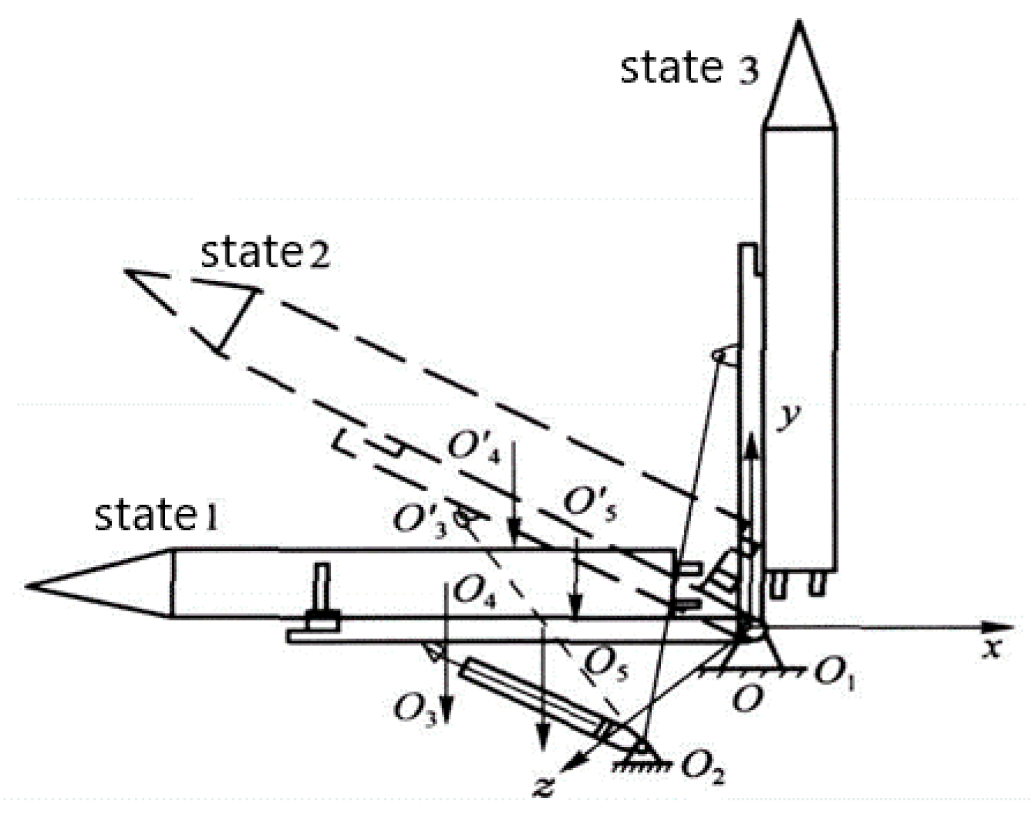
2. Model of Electromechanical Servo System

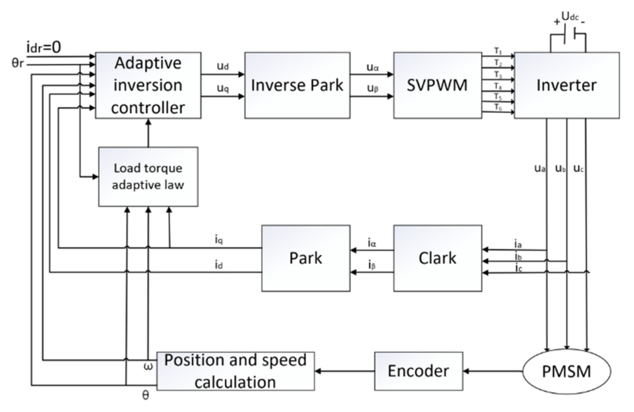
2.1. Mathematical Model of PMSM

For PMSM vector control system, it is very convenient to analyze the dynamic and steady-state performance in d-q coordinate system. The following is the mathematical model of surface mounted permanent magnet synchronous motor in synchronous rotating coordinate system:

$$\{\begin{array}{l}L\frac{d{i}_d}{dt}=-R_s{i}_d+n_p\omega L{i}_q+u_d\\ L\frac{d{i}_q}{dt}=-R_s{i}_q-n_p\omega L{i}_d-n_p\varphi \omega +u_q\\ J\frac{d\omega }{dt}=\tau -{\tau }_L=n_p\varphi i_q-{\tau }_L\\ \frac{d\theta }{dt}=\omega \end{array}$$

(1)

$$\tau =n_p\varphi i_q$$

(2)

where $i_d$ and $i_q$ are the stator current of d-axis and q-axis, respectively; $u_d$ and $u_q$ are the stator voltage of d-axis and q-axis, respectively; $\theta$ is the rotor angle; $\omega$ is the mechanical angular velocity of the rotor; $\tau$ and ${\tau }_L$ is electromagnetic torque and load torque, respectively; J is the moment of inertia; L is the stator inductance; $R_s$ is the stator phase resistance; $n_p$ is the polar logarithm; $\varphi$ is the permanent magnet flux linkage of motor.

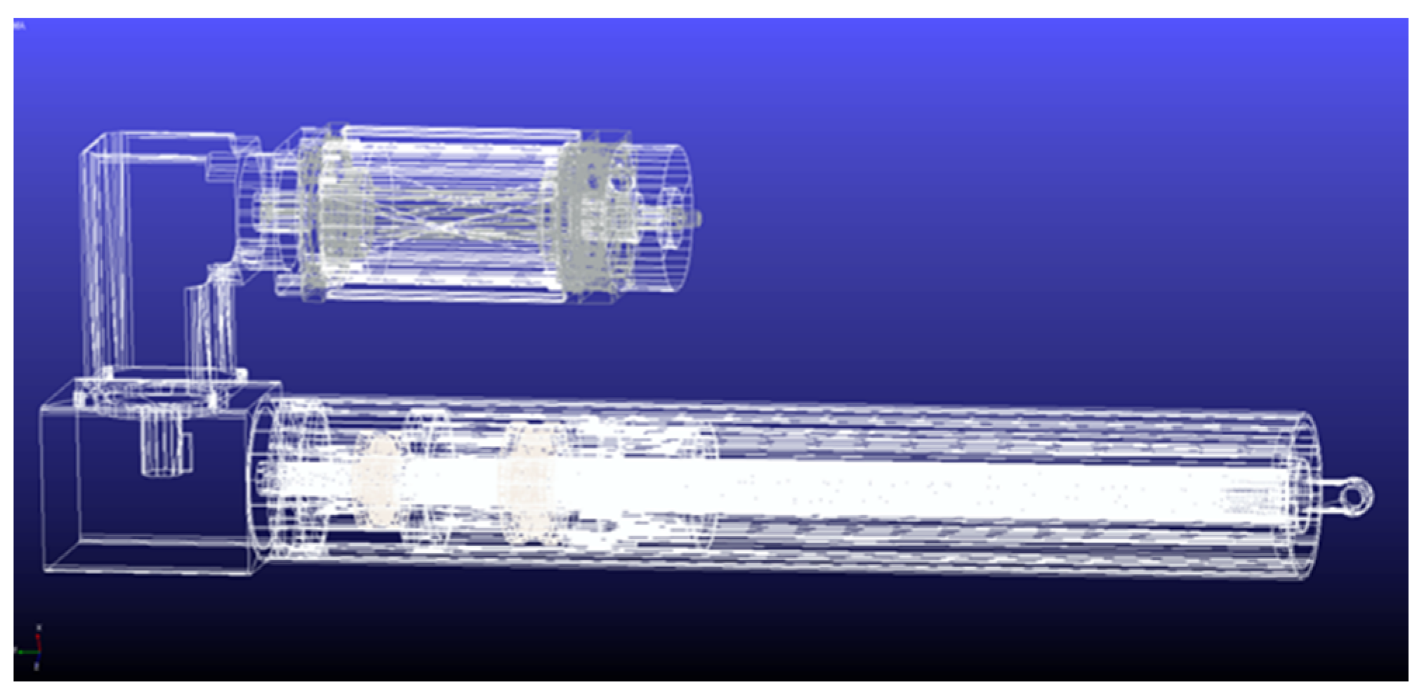
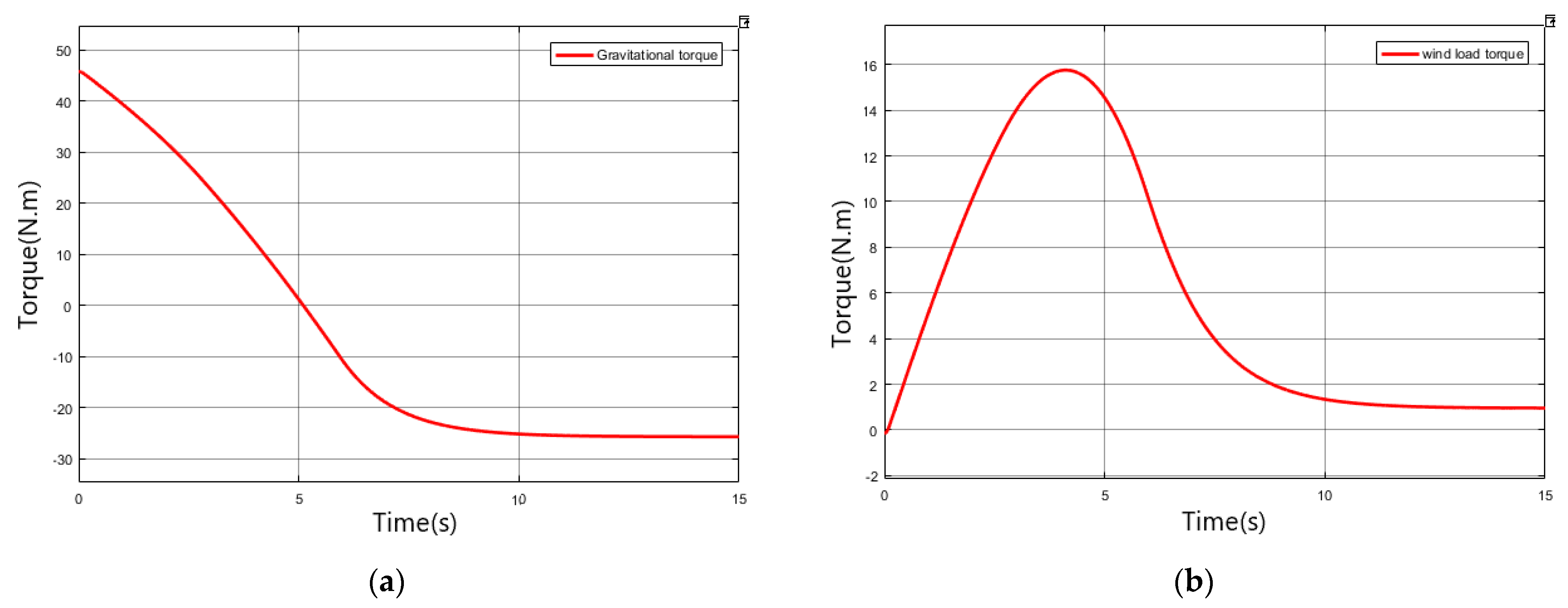
2.2. Dynamic Model of Planetary Roller Screw

In this paper, the three-stage planetary roller screw is used as the actuator of EMA to measure the performance indexes of the three-stage planetary roller screw, mainly including displacement acceleration, velocity, and displacement.

$$l={{\displaystyle \int }}_0^{t}n\left(P_{h1}+P_{h2}+P_{h3}\right)dt={{\displaystyle \int }}_0^t\frac{\omega \left(t\right)}{2\pi \cdot i}\left(P_{h1}+P_{h2}+P_{h3}\right)dt$$

(3)

where n is the speed of the main screw, t is the working time, i is the reduction ratio, and $\omega \left(t\right)$ is the rotational angular speed of the motor.

By deriving the displacement, the velocity v of the three-stage planetary roller screw is obtained as:

$$v=\frac{dl}{dt}=\frac{\omega \left(t\right)}{2\pi \cdot i}\left(P_{h1}+P_{h2}+P_{h3}\right)$$

(4)

By deriving the velocity, the expression of acceleration, a, is:

$$a=\frac{dv}{dt}=\frac{\alpha \left(t\right)}{2\pi \cdot i}\left(P_{h1}+P_{h2}+P_{h3}\right)$$

(5)

where α(t) is the rotational angular acceleration of the motor.

For the bearing problem of the three-stage planetary roller screw, the screws at all levels are distributed the load according to the structure. The load distribution law inside a certain level of screw is the same as that of the single-stage planetary roller screw. The axial load of the screw at all levels is equal, which is equal to the load F of the screw. Then, we obtain:

$$F_1=F_2=F_3=F$$

(6)

The three-stage hollow screw only needs to drive the nut of this stage to transmit motion, and the transmission efficiency is ${\eta }_3$. The torque of the three-stage hollow screw is:

$$T_3=\frac{F{P}_{h3}}{2\pi {\eta }_3}$$

(7)

The two-stage hollow screw not only provides torque for the axial movement of the two-stage nut, but also drives the rotation of the three-stage hollow screw. It can be regarded as the screw transmission with P_h2 + P_h3, and its transmission efficiency is ${\eta }_2$. Then, the torque of the secondary hollow screw is:

$$T_2=\frac{F\left(P_{h2}+P_{h3}\right)}{2\pi {\eta }_2}$$

(8)

Similarly, it can be seen that the primary main screw can be regarded as the screw transmission with lead of P_h1 + P_h2 + P_h3, and its transmission efficiency is ${\eta }_1$. The torque of the primary main screw is:

$$T_1=\frac{F\left(P_{h1}+P_{h2}+P_{h3}\right)}{2\pi {\eta }_1}$$

(9)

The mathematical model of mechanical transmission part is mainly divided into two parts: the linear speed of screw and the thrust of electromechanical actuator. Let the reduction ratio of the reducer be i, the lead of the planetary roller screw be p, and the angular speed of the motor rotor be ${\omega }_m$. The speed of the screw can be expressed as:

$$v=\frac{ip{\omega }_m}{2\pi }$$

(10)

Set the thrust of electromechanical actuator as $F_m$, $\eta$ is the efficiency of the actuator, and the torque of the motor can be expressed as:

$$T_m=\frac{F_{m}p}{2\pi i\eta }$$

(11)

In this paper, large vertical equipment is analyzed as the application object of EMA. Figure 1 shows the schematic diagram of vertical equipment. Taking this working condition as an example, the mathematical models of load torque and wind load torque of vertical equipment are analyzed and established.

When the system is in state 1, set the angle between the line between the load center of mass O₄ and the vertical rotation point O₁ and the horizontal plane as θ₀, then when the vertical mechanism is in state 2 at time t, the angle between the line between the load center of mass O₄′ and the vertical rotation point O₁ and the horizontal plane:

$${\theta }^{\prime }\left(t\right)={\theta }_0+\theta \left(t\right)$$

(12)

At this time, the load gravity torque $M_G\left(t\right)$ that the load acting on the mechanism rotation point O₁ due to its own gravity is:

$$M_G\left(t\right)=G\cdot L_{G}cos\left({\theta }_0+\theta \left(t\right)\right)$$

(13)

where G is the load gravity, and L_G is the length of O₁ O₄ from the load centroid to the vertical rotation point.

For vertical erection equipment, wind load [30] is a factor that must be considered in system design. When studying the role of wind, except for the application in complex terrain, the influence of vertical wind on the system is not generally considered, and it is considered that the wind speed is parallel to the ground. When considering the influence of wind in system design, the wind field is usually modeled, and the wind is divided into two parts: steady wind and gust. The variation of steady wind along the height is represented by wind profile. The gust factor method is used to estimate the load caused by gust in the system design.

The wind pressure, derived after considering the nature of the wind, the shape of the wind-receiving structure, and the position height, is called the calculated wind pressure, q_i, and its value can be obtained from the following formula:

$$q_i=q{C}_x{R}_H\beta$$

(14)

where q is the rated wind pressure; C_x is the aerodynamic drag coefficient; R_H is the correction coefficient of wind pressure increasing with height; β is the dynamic coefficient for calculating gust.

The calculation formula of rated wind pressure is:

$$q=\frac{\rho v^2}{2}$$

(15)

where ρ is the air density at a certain temperature; v is the given wind speed.

The variation law of average wind speed along height can be approximated by the following logarithmic function:

$$\frac{v\left(H\right)}{v\left(H_1\right)}={\left[\frac{H}{H_1}\right]}^{\alpha }$$

(16)

where v(H) is the average wind speed at heigh H; v(H₁) is the average wind speed at the standard height H₁ (generally 10 m); α is the ground roughness coefficient.

The aerodynamic resistance coefficient C_x is related to the structure and shape of the equipment. When considering the effect of wind on the load, there is not only the pressure on the windward side, but also the pressure reduction on the back, and its effect is equivalent to the pressurization on the windward side. The distribution of pressure coefficient along the load surface is uneven. When considering the total wind load acting on the load, the total aerodynamic resistance coefficient can be taken as 0.6. The dynamic coefficient β of gust is related to the structure, and the structure is taken according to its natural vibration period between 1.22 and 1.75. The correction coefficient R_H of wind pressure increasing with height can be obtained by looking up the table. Finally, the wind load can be calculated by the following formula:

$$F_w={\displaystyle \sum }{q}_i{A}_i$$

(17)

where A_i is the calculated windward area.

Considering the extreme case of vertical wind load, with wind direction parallel to the vertical plane, the calculated wind pressure acting at a certain height on the load at time t is as follows:

$$q_i\left(t\right)=\frac{1}{2}\rho {\left[{\left(\frac{H}{H_1}\right)}^{\alpha }v\left(H_1\right)C_x{R}_H\beta \right]}^2$$

(18)

$$H=H_0+xsin\theta \left(t\right)$$

(19)

where H₀ is the vertical distance between the vertical rotation center O₁ and the ground; x is the distance from the wind pressure calculation point along the axial direction of the load to the rotation point.

Wind load acting on the load at time t:

$$F_w\left(t\right)={\displaystyle \int }{q}_i\left(t\right)d{A}_i\left(t\right)={\displaystyle \int }{q}_i\left(t\right)Dsin\theta \left(t\right)dx$$

(20)

where D is the effective diameter of the windward side of the load.

The torque generated by the wind load acting on the load at time t is:

$$M_w\left(t\right)={\displaystyle \int }{q}_i\left(t\right)xsin\theta \left(t\right)d{A}_i\left(t\right)$$

(21)

3. Adaptive Inversion Control

3.1. Design of Adaptive Inversion Controller

This paper adopts $i_d=0$, and the control realizes the decoupling control and position tracking control of PMSM. Figure 2 is the system control block diagram. The PMSM control system includes adaptive backstepping position controller, load torque adaptive law, coordinate transformation module, SVPWM module, inverter, and PMSM. The reference position is ${\theta }_r$, and the given d-axis current is $i_{dr}=0$; the main purpose of the controller is to obtain the appropriate control voltage to realize the position tracking control.

According to the inversion control principle, the position error and its first derivative are defined as:

$$e_{\theta }=\theta -{\theta }_r$$

(22)

$${\dot{e}}_{\theta }=\dot{\theta }-{\dot{\theta }}_r=\omega -{\dot{\theta }}_r$$

(23)

Introduce speed virtual control quantity:

$${\omega }_d^{*}={\dot{\theta }}_r-k{e}_{\theta },k>0$$

(24)

Then, ${\dot{e}}_{\theta }=k{e}_{\theta }$ can be obtained by combining Formulas (22) and (23). Define the speed tracking error and its first derivative as:

$$e_{\omega }=\omega -{\omega }_d^{*}$$

(25)

$${\dot{e}}_{\omega }=\dot{\omega }-{\dot{\omega }}_d^{*}$$

(26)

Because the load torque is unknown, we define the Lyapunov function as:

$$V_1=\frac{1}{2}{e}_{\omega }^2+\frac{1}{2}{\gamma }_1^{-1}{\tilde{\tau }}_L^2$$

(27)

where ${\gamma }_1$ is a strictly positive definite adaptive gain, ${\tilde{\tau }}_L={\tau }_L-{\widehat{\tau }}_L$ is the load error, and ${\widehat{\tau }}_L$ represents the estimated value of the load torque, ${\tau }_L$. Although the load torque is an unknown variable, if the sampling interval changes fast enough compared with the load disturbance time, the disturbance model can be considered as ${\dot{\tau }}_L=0$. So, the derivative of the load torque error is ${\dot{\tilde{\tau }}}_L=-{\dot{\widehat{\tau }}}_L$.

According to the above analysis, the first derivative of Equation (27) is:

$${\dot{V}}_1=e_{\omega }{\dot{e}}_{\omega }+{\gamma }_1^{-1}{\tilde{\tau }}_L{\dot{\tilde{\tau }}}_L=e_{\omega }\left(\dot{\omega }-{\dot{\omega }}_d^{*}\right)-{\gamma }_1^{-1}{\tilde{\tau }}_L{\dot{\tilde{\tau }}}_L$$

(28)

According to the inversion control principle, the virtual control current $i_{qr}$ and q-axis current error $e_{iq}$ are introduced:

$$\{\begin{array}{l}{i}_{qr}=\frac{J}{n_p\varphi }\left(\alpha +{\dot{\omega }}_d^{*}\right)\\ e_{iq}=i_q-i_{qr}\end{array}$$

(29)

where $\alpha$ is the stabilization function, which can make $e_{iq}$ asymptotically stable. Combining Equations (1), (24), (28) and (29), we can obtain:

$${\dot{V}}_1=\frac{1}{J}{n}_p\varphi e_{\omega }{e}_{iq}+e_{\omega }\underset{-k_1{e}_{\omega }}{\underbrace{\left(\alpha -\frac{1}{J}{\widehat{\tau }}_L\right)}}+{\tilde{\tau }}_L\underset{-k_2{\tilde{\tau }}_L}{\underbrace{\left(-\frac{e_{\omega }}{J}-{\gamma }_1^{-1}{\dot{\widehat{\tau }}}_L\right)}}$$

(30)

where the feedback gain is $k_1>0,k_2>0$.

The stabilization function $\alpha$ and the load torque adaptive law ${\dot{\widehat{\tau }}}_L$ are selected as:

$$\alpha =-k_1{e}_{\omega }+\frac{1}{J}{\widehat{\tau }}_L$$

(31)

$${\dot{\widehat{\tau }}}_L={\gamma }_1{k}_2{\tilde{\tau }}_L-\frac{1}{J}{\gamma }_1{e}_{\omega }$$

(32)

Equation (28) can now be transformed into:

$${\dot{V}}_1=\frac{1}{J}{n}_p\varphi e_{\omega }{e}_{iq}-k_1{e}_{\omega }^2-k_2{\tilde{\tau }}_L^2$$

(33)

Before proceeding to the next design step, we need to clarify the derivation process of the load disturbance estimation ${\widehat{\tau }}_L$. Through the mathematical model of PMSM given by Equation (1), we know that

$${\tau }_L=n_p\varphi i_q-J\dot{\omega }$$

(34)

Bring Equation (34) into (33) and rearrange it to obtain:

$${\dot{\widehat{\tau }}}_L=-{\gamma }_1{k}_{2}J\dot{\omega }+{\gamma }_1\left[\frac{1}{J}{e}_{\omega }+k_2\left(n_p\varphi i_q-{\widehat{\tau }}_L\right)\right]$$

(35)

Integrating both sides of (35) gives:

$${\widehat{\tau }}_L=-{\gamma }_1{k}_{2}J{{\displaystyle \int }}_{\omega \left(0\right)}^{\omega \left(t\right)}\dot{\omega }+{\gamma }_1{{\displaystyle \int }}_0^t\left[\frac{1}{J}{e}_{\omega }+k_2\left(n_p\varphi i_q-{\widehat{\tau }}_L\right)\right]dt$$

(36)

Arranged to obtain:

$$\begin{array}{c}{\widehat{\tau }}_L=-{\gamma }_1{k}_{2}J{{\displaystyle \int }}_{\omega \left(0\right)}^{\omega \left(t\right)}\dot{\omega }+{\tau }_{L0}\\ {\dot{\tau }}_{L0}={\gamma }_1\left[\frac{1}{J}{e}_{\omega }+k_2\left(n_p\varphi i_q-{\widehat{\tau }}_L\right)\right]\end{array}$$

(37)

Among them, the feedback gain only exists in the adaptive law, which makes the adjustment simpler. The load torque adaptive law is similar to the nonlinear reduced-order disturbance observer, which can realize fast and accurate load disturbance estimation.

Substituting Equation (31) into Equation (29), we can obtain the current expression for the q-axis:

$$i_{qr}=\frac{J}{n_p\varphi }\left[-k_1\left(\omega -{\omega }_d^{*}\right)+\frac{1}{J}{\widehat{\tau }}_L+{\dot{\omega }}_d^{*}\right]$$

(38)

Taking the derivative of both sides gives:

$${\dot{i}}_{qr}=\frac{J}{n_p\varphi }\left[-k_1\left(\frac{1}{J}{n}_p\varphi i_q-\frac{1}{J}{\tau }_L\right)+k_1{\dot{\omega }}_d^{*}+\frac{1}{J}\left({\gamma }_1{k}_2{\tilde{\tau }}_L-\frac{{\gamma }_1}{J}{e}_{\omega }\right)+{\ddot{\omega }}_d^{*}\right]$$

(39)

Next, we need to choose the appropriate voltage so that $e_{iq}\to 0$. Define the Lyapunov function V₂ as:

$$V_2=V_1+\frac{1}{2}{e}_{iq}^2$$

(40)

According to Equations (1), (29), (33) and (39), we can obtain the derivative of V₂ as:

$$\begin{gathered} {\dot{V}}_2=-k_1{e}_{\omega }{}^2-k_2{\tilde{\tau }}_L{}^2-\frac{1}{n_p\varphi }\left(k_1+{\gamma }_1{k}_2\right)e_{iq}{\tilde{\tau }}_L+e_{iq} \\ \left[\frac{n_p\varphi }{J}{e}_{\omega }-\frac{R_s}{L_q}{i}_q-n_p\omega i_d-\frac{n_p\varphi }{L_q}\omega +\frac{u_q}{L_q}+k_1{i}_q-\frac{k_1}{n_p\varphi }{\widehat{\tau }}_L-\frac{J}{n_p\varphi }{k}_1{\dot{\omega }}_d^{*}+\frac{{\gamma }_1}{J{n}_p\varphi }{e}_{\omega }-\frac{J}{n_p\varphi }{\ddot{\omega }}_d^{*}\right] \end{gathered}$$

(41)

In the formula, the last term is changed to $-k_3{e}_{iq}$, and k₃ is the positive feedback gain. According to Formula (41), we can obtain the vacancy rate u_q as:

$$u_q=L\left[-k_3{e}_{iq}-\left(\frac{n_p\varphi }{J}+\frac{{\gamma }_1}{J{n}_p\varphi }\right)e_{\omega }+\left(\frac{R_s}{L_q}-k_1\right)i_q+n_p\omega i_d+\frac{n_p\varphi }{L_q}\omega +\frac{k_1}{n_p\varphi }\left({\widehat{\tau }}_L+J{\dot{\omega }}_d^{*}\right)+\frac{J}{n_p\varphi }{\ddot{\omega }}_d^{*}\right]$$

(42)

Bringing Equation (42) into (41), we can obtain:

$${\dot{V}}_2=-k_1{e}_{\omega }{}^2-{\left(\sqrt{\frac{k_2}{2}}{\tilde{\tau }}_L+\frac{n}{\sqrt{2k_2}}{e}_{iq}\right)}_{}^2-{\left(\sqrt{\frac{k_2}{2}}{\tilde{\tau }}_L+\frac{m}{\sqrt{2k_2}}{e}_{iq}\right)}^2-\left(k3-\frac{m^2+n^2}{2k_2}\right)e_{iq}{}^2$$

(43)

where $m=k_1/n_p\varphi$, $n={\gamma }_1{k}_2/n_p\varphi$. When $k_3\ge \left(m^2+n^2\right)/2k_2$, ${\dot{V}}_2$ is negative definite.

Define the d-axis current error e_id as:

$$e_{id}=i_d-i_{dr}$$

(44)

where i_dr = 0. By deriving from the above formula:

$${\dot{e}}_{id}={\dot{i}}_d-{\dot{i}}_{dr}=-\frac{R_s}{L}{i}_d+n_p\omega i_q+\frac{1}{L}{u}_d$$

(45)

The Lyapunov function is defined as:

$$V_3=\frac{1}{2}{e}_{id}^2$$

(46)

$${\dot{V}}_3=e_{id}\underset{-k_4{e}_{id}}{\underbrace{\left(-\frac{R_s}{L}{i}_d+n_p\omega i_q+\frac{1}{L}{u}_d\right)}}$$

(47)

where feedback gain $k_4>0$, the selected control rate u_d is:

$$u_d=-L{k}_4{e}_{id}+R_s{i}_d-L{n}_p\omega i_q$$

(48)

Equation (47) can be changed into:

$${\dot{V}}_3=-k_4{e}_{id}{}^2<0$$

(49)

3.2. Design of Luenberger Observer

The Luenberger observer is an observer model based on the mathematical model of PMSM. The estimated state variables are modified according to the error feedback to achieve the purpose of error convergence and state reconstruction. The Luenberger observer has the advantages of fast response and high observation accuracy. We use position error feedback to construct the Luenberger observer:

$$\{\begin{array}{c}\dot{\widehat{\theta }}=\widehat{\omega }+l_1\left(\theta -\widehat{\theta }\right)\\ \dot{\widehat{\omega }}=\frac{n_p}{J}\varphi i_q-\frac{{\widehat{\tau }}_L}{J}+l_2\left(\theta -\widehat{\theta }\right)\\ {\dot{\widehat{\tau }}}_L=l_3\left(\theta -\widehat{\theta }\right)\end{array}$$

(50)

where $\tilde{\theta }=\left(\theta -\widehat{\theta }\right)$, $\tilde{\omega }=\omega -\widehat{\omega }$, ${\tilde{\tau }}_L={\tau }_L-{\widehat{\tau }}_L$.

The error dynamic equation can be obtained from Equation (50):

$$\left[\begin{array}{c}\dot{\tilde{\theta }}\\ \dot{\tilde{\omega }}\\ {\dot{\tilde{\tau }}}_L\end{array}\right]=\left[\begin{array}{ccc}-l_1& 1& 0\\ -l_2& 0& -\frac{1}{J}\\ -l_3& 0& 0\end{array}\right]\left[\begin{array}{c}\tilde{\theta }\\ \tilde{\omega }\\ {\tilde{\tau }}_L\end{array}\right]$$

(51)

The characteristic equation of the observer can be obtained from Equation (51):

$$s^3+l_1{s}^2+l_{2}s-\frac{l_3}{J}=0$$

(52)

According to the Routh stability criterion, the system (51) is asymptotically stable if and only if $l_1>0$, $l_2>0$. Suppose the pole of the observer is $S_p\left(S_p<0\right)$, then the parameter is $l_1=-3S_p$, $l_2=3S_p^2$, $l_3=J{S}_p^3-J{l}_1{l}_2<l_3<0$.

3.3. Stability Analysis

The stability of the whole system depends on the stability of each subsystem. The Lyapunov function of the whole control system is defined as:

$$V=\frac{1}{2}{e}_0^2+V2+V3=\frac{1}{2}{e}_0^2+\frac{1}{2}{e}_{\omega }^2+\frac{1}{2}{\gamma }_1^{-1}{\tilde{\tau }}_L^2+\frac{1}{2}{e}_{iq}^2+\frac{1}{2}{e}_{id}^2$$

(53)

Derivating the Lyapunov function gives:

$$\dot{V}=-k{e}_{\theta }^2-k_1{e}_{\omega }^2-k_4{e}_{id}^2-{\left(\sqrt{\frac{k_2}{2}}{\tilde{\tau }}_L+\frac{n}{\sqrt{2k_2}}{e}_{iq}\right)}^2-{\left(\sqrt{\frac{k_2}{2}}{\tilde{\tau }}_L+\frac{m}{\sqrt{2k_2}}{e}_{iq}\right)}^2-\left(k_3-\frac{m^2+n^2}{2k_2}\right)e_{iq}^2<0$$

(54)

where it is guaranteed that $k_3\ge \frac{m^2+n^2}{2k_2}$. $\dot{V}=0$ if, and only if, $e_{\theta }=e_{\omega }=e_{id}=e_{iq}={\tilde{\tau }}_L=0$. Because $V$ is positive definite and $\dot{V}$ is negative definite, the whole system is asymptotically stable according to Lyapunov stability principle and Lasalle invariance principle.

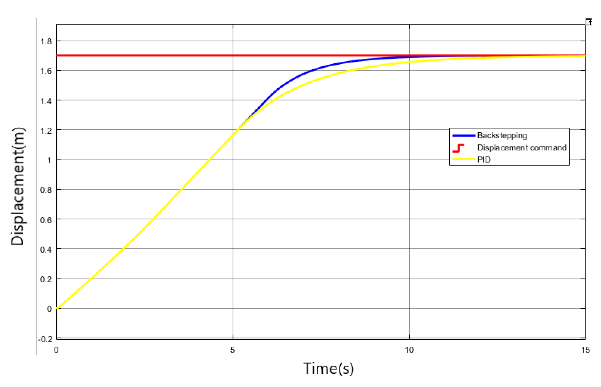
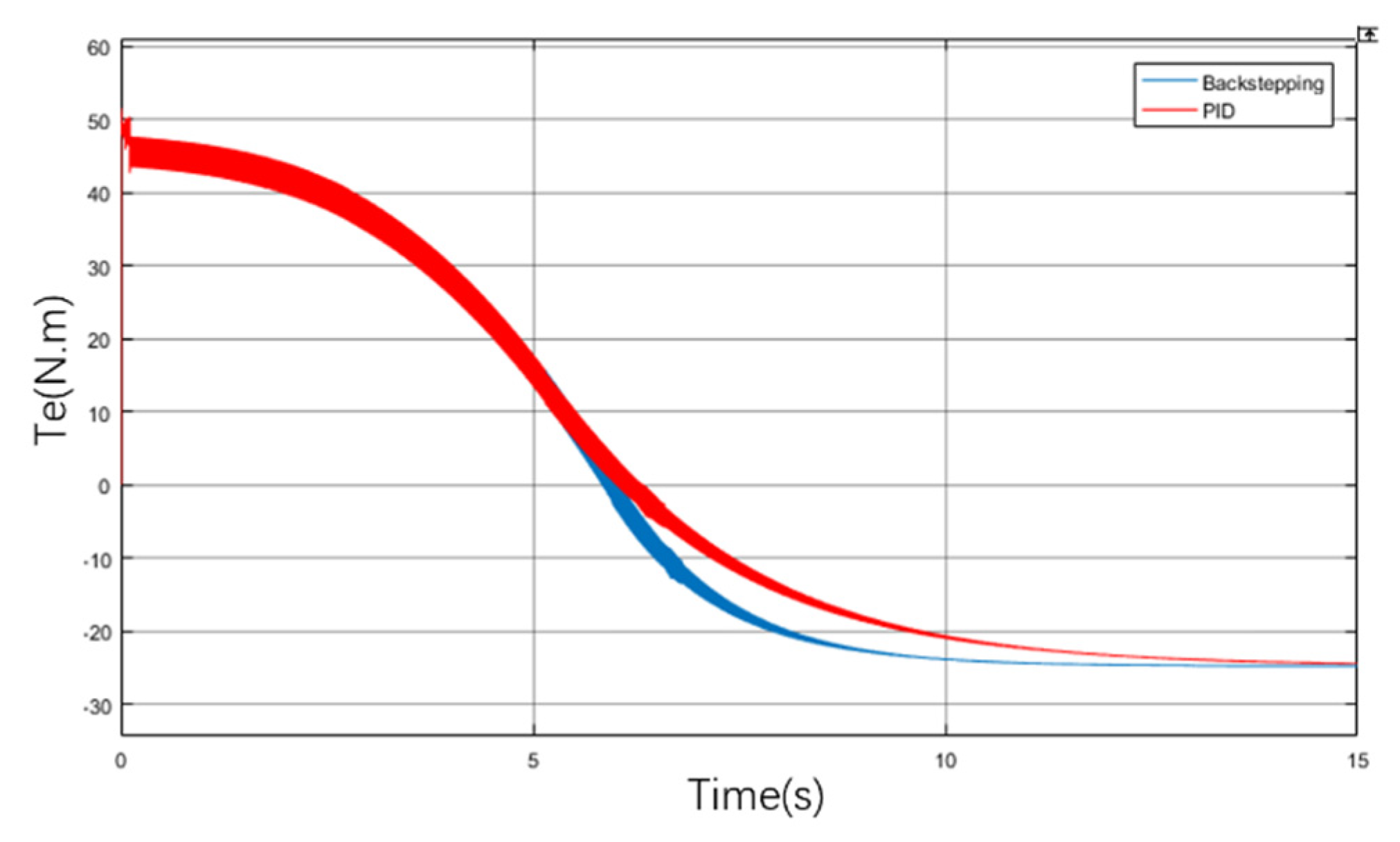
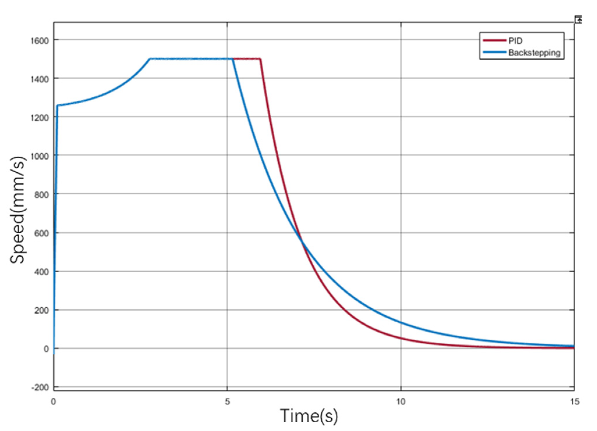
3.4. Joint Simulation Test

In this paper, the motion model of the multilevel electromechanical servo system was established using ADAMS (The Mechanical Dynamics, Inc., Ann Arbor, MI, USA) software (as shown in Figure 3), and the overall performance of the system combined with the mechanical part was analyzed through co-simulation with Simulink, which is a simulation package for MATLAB^® (The MathWorks, Inc., Natick, MA, USA), and ADAMS, so as to verify the effectiveness and reliability of the controller designed in this paper.

The motor parameters used in the simulation in this paper were as follows: d-q axis inductance was 0.395 mH; stator resistance was 0.0433 Ω; moment of inertia was 0.0024 kg·m²; number of pole pairs was 4; permanent magnet flux was 0.1192 V·s. Calculate the actual load of the system according to the mathematical model of gravity torque and wind load torque. When calculating the gravity torque, the weight of the heavy object was set to 10 tons. The parameters used in calculating the wind load torque are shown in

Table 1. Calculation parameters of wind load torque.

Parameters	Parameters Value
aerodynamic drag coefficient Cx	0.6
correction factor RH	1.52
gust dynamic coefficient β	1.5
roughness index α	0.12
local wind speed v (m/s)	2.5
air density ρ (kg/m3)	1.35

(assuming that the application site is Urumqi and that the local temperature is 20 °C).

The mathematical model for deriving the load torque is simulated in Simulink and the results are shown in Figure 4. Figure 4a is the part of the gravitational torque. It can be seen from the figure that the torque first decreases with time during the erection process, and then the reverse increases. Figure 4b is the wind load torque part, it can be seen from the figure that the torque increases first and then decreases with time during the erection process. Take the sum of the two parts of the torque as the load torque of the system.

Given the displacement command of 1.7 m and the simulation time of 15 s, the load torque is the sum of the calculated gravity torque and the wind load torque. The simulation comparison results of the electromechanical actuation system under the traditional PID and adaptive inversion controller are shown in Figure 5. When the displacement is 1.7 m, the system can reach the system displacement command in 9.8 s under the adaptive inversion controller with a relative error of 0.012%, while it is stable in 12.4 s under the traditional PID control, with a relative error of 0.71%.

The load torque is composed of the two parts of torque in Figure 4. The load of the system according to the load torque is shown in Figure 6. The figure shows that the torque provided by the motor first decreases to zero and then increases in the opposite direction during the system operation.

Figure 7 is a graph showing the speed comparison of the motor when the electromechanical actuation system is running. It can be seen that the adaptive inversion method can reach the target command faster with higher precision, indicating that it has better dynamic performance and verifies the feasibility and reliability of the design.

4. Experimental Research

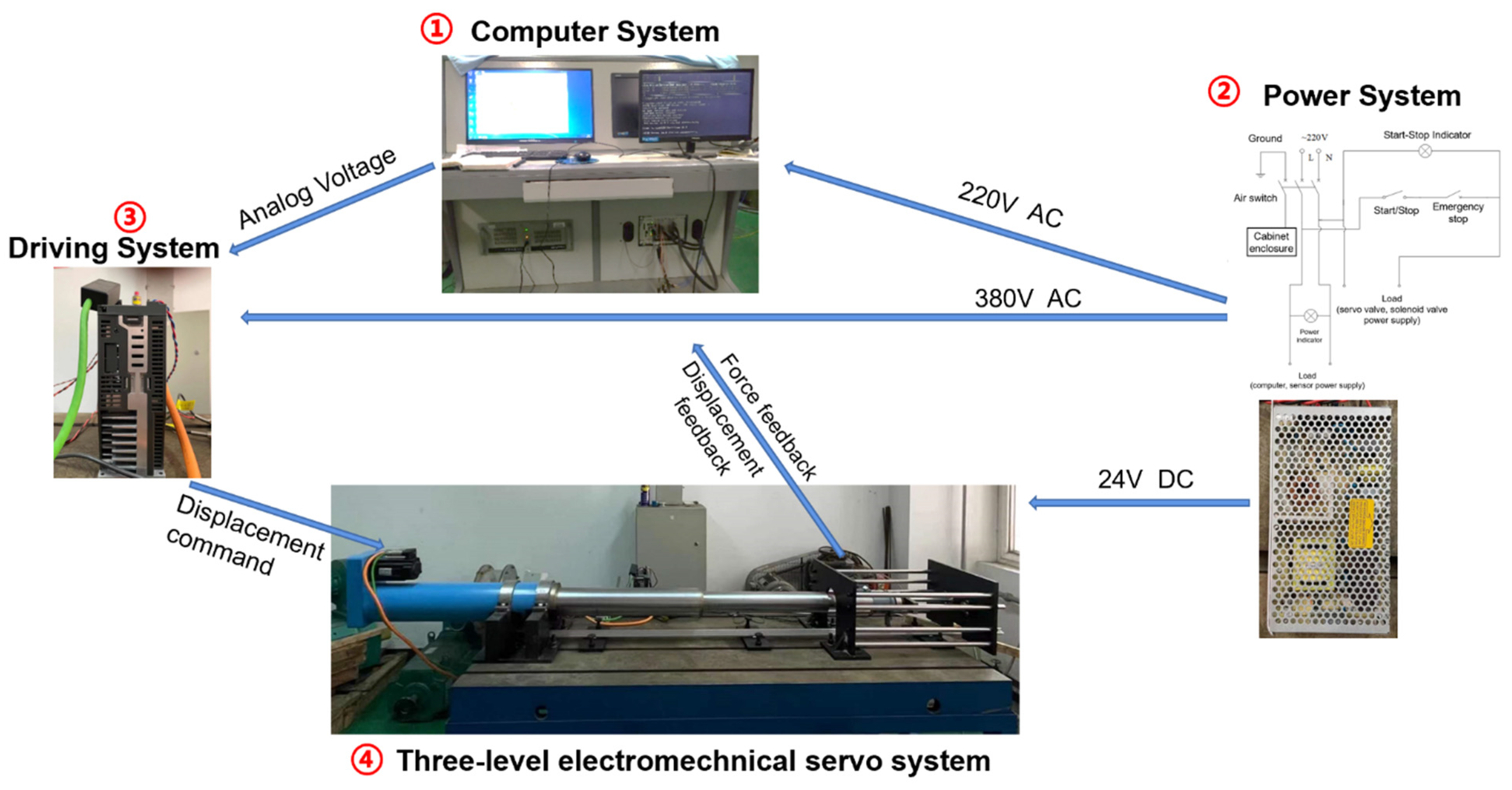
4.1. Experiment Platform

This paper builds a three-level electromechanical servo system test bench based on LABVIEW, as shown in Figure 8, the test bench consists of four parts: ① computer system, ② power supply system, ③ driving system, and ④ electromechanical servo system. ② Supply required voltage to ①③④. After the system runs, the sensor in ④ feeds back the force and displacement signals to ①, and outputs the analog voltage to ③ after being calculated by the control algorithm in ①, so as to generate the three-phase voltage corresponding to the target displacement to control the movement of ④. The self-adaptive inversion control technology designed in this paper has high precision requirements for the motion of the control object, and the small- and medium-sized servo motors were selected as the control object. According to the motion control index of the test bench, the jarrett AC servo motor was selected with a rated power of 820 W, a rated speed of 3000 rpm, and a rated torque of 2.6 N·m. The lead of the actuating cylinder used in the test was 5 mm, the number of stages was three, the maximum stroke was 1800 mm, the maximum extension speed was 100 mm/s, and it could push a load of 800 N.

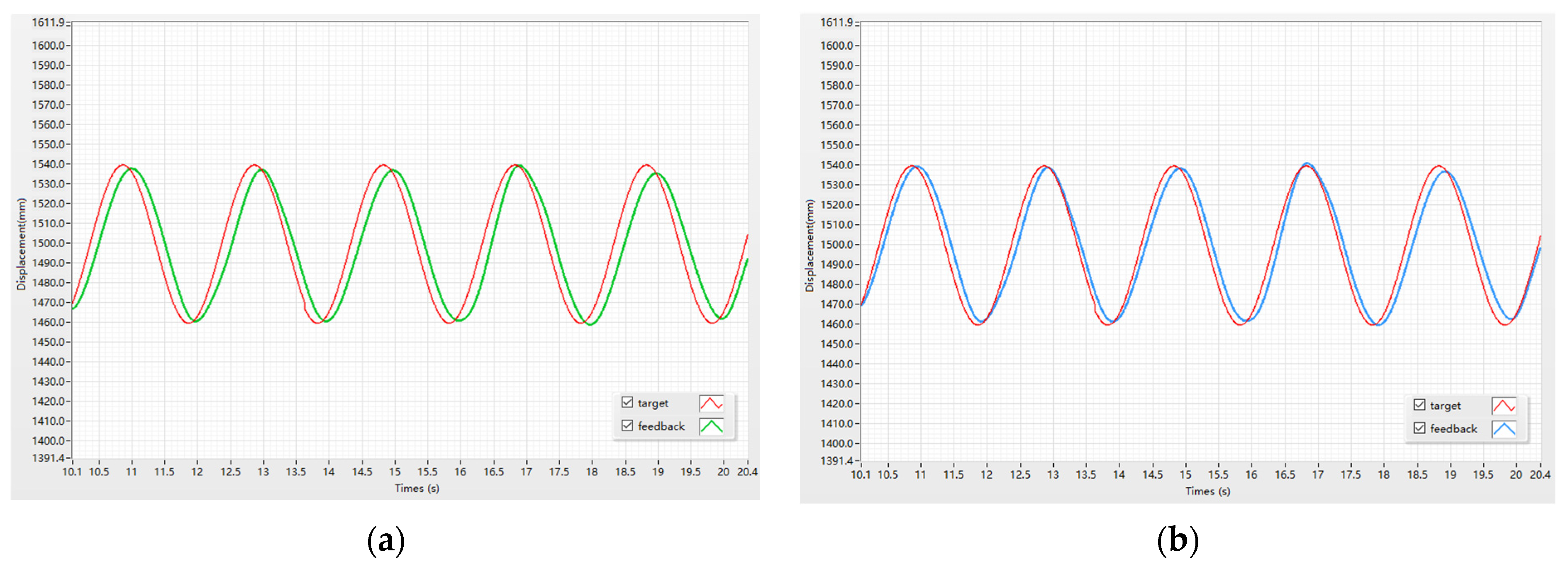
4.2. Experimental Results

The dynamic performance of the motor system represents the advantages and disadvantages of the motor control performance. In this study, the step signal tracking test was firstly carried out. During the movement process, the multilevel EMA works under variable load conditions. The test used a spring device to simulate variable load loading of multistage EMA. After the system was powered on, the upper computer gave a step displacement command when the lateral spring gave a constant force of 150 N. Since the spring of the loading device had a maximum deformation constraint, the load step displacement command could not exceed the maximum deformation range. Here, the amplitudes were set to 100 mm, 200 mm, 400 mm, and 800 mm, respectively. The control algorithm adopted traditional PID and adaptive inversion method, respectively, to read the feedback signal of the displacement sensor. The test results are shown in

Table 2. Time domain indicators of multistage electromechanical servo system.

Step Displacement Command (mm)	Traditional PID Control		Adaptive Inversion Control
	Average Adjustment Time	Average Overshoot	Average Adjustment Time	Average Overshoot
	(s)	(mm)	(s)	(mm)
100	3.3	1.1	2.6	0.3
200	4.2	2	3.1	0.4
400	6.8	1.2	5.1	0.4
800	11.5	1.8	9.0	0.3

.

The analysis shows that, under the step displacement command of 100 mm, 200 mm, 400 mm, and 800 mm, the adaptive inversion control had a significant decrease in the average adjustment time compared with the traditional PID, and the decrease rates were 21.2%, 26.2%, 23.5%, and 21.7%, respectively. In terms of the average overshoot, the reduction ranges reached 72.7%, 80%, 66.7%, and 83.3%, which verifies that the adaptive inversion control method designed in this paper can significantly improve the fast response of the loading system, reduce the system overshoot, and improve loading accuracy.

Afterwards, the sinusoidal signal tracking experiment was carried out. The sinusoidal test can effectively test the followability of the controlled target to the command and measure the control effect of the adaptive inversion strategy. The output end of the multilevel electromechanical servo system was connected to a spring load, the system was powered on, the host computer gave a sinusoidal displacement command, and set the corresponding offset, so that the EMA ran in the range of 1100~1900 mm, 1300~1700 mm, 1400~1600 mm, 1420~1580 mm, respectively. Inside, the corresponding frequencies were 0.05 Hz, 0.1 Hz, 0.2 Hz, and 0.5 Hz, respectively. Figure 9 shows the comparison of the traditional PID and the adaptive inversion method at a frequency of 0.5 Hz, and the comparison data at different frequencies are summarized in

Table 3. Displacement following performance parameters of multilevel electromechanical system.

Sinusoidal Displacement Command (mm)	Frequency (Hz)	Traditional PID Control		Adaptive Inversion
		Lag Time (s)	Amplitude Decay	Lag Time (s)	Amplitude Decay
1100~1900	0.05	2.2	9.4%	1.2	4.9%
1300~1700	0.1	1.2	6.8%	0.5	3.5%
1400~1600	0.2	0.5	3.7%	0.3	2.8%
1460~1540	0.5	0.2	1.7%	0.1	0.9%

.

The analysis shows that, when the system displacement closed loop adopts the adaptive inversion control strategy, the multilevel electromechanical servo system has better follow-up performance. Under the same command, its lag time and amplitude decay are better than the traditional PID strategy.

5. Conclusions

(1)

In this paper, an adaptive inversion control method is proposed for the nonlinear problem of the multilevel electromechanical servo system. Through joint simulation with Simulink and ADAMS software, the displacement, torque, and speed results of a multistage electromechanical servo system under an adaptive inversion controller and a traditional PID controller are compared, to verify the feasibility and reliability of the designed controller. The designed control algorithm was debugged on the experimental platform, and the system step signal tracking and sinusoidal signal tracking tests were carried out. The test results verify that the designed adaptive inversion multistage EMA driving algorithm can respond quickly, has better tracking performance, and has better robustness and stability than the traditional PID controller.

(2)

Next, the future work is to replace the analog sensor with a digital sensor and change the loading mode to improve the experimental accuracy.

References

1. Feng, S.; Meng, X.; Li, G. The Superior Election of Antiaircraft Missile Firing Mode Based on Advanced ADC. Guid. Fuze 2006. [Google Scholar]
2. Li, X.; Liu, G.; Song, C. Rigid-Body Dynamic Analysis of Multi-Stage Planetary Roller Screw Mechanism. J. Northwest. Polytech. Univ. 2020, 38, 1001–1009. [Google Scholar] [CrossRef]
3. Li, Y.; Yan, X. The Perspective and Status of PMSM Electrical Servo System. Micromotors 2021, 34, 30–33. [Google Scholar]
4. Chen, X. Research on Control Strategy of Electromechanical Actuation Servo System for More Electric Aircraft; Northwestern Polytechnical University: Xi’an, China, 2016. [Google Scholar]
5. Yuan, L.; Hu, B.; Wei, K. Control Principle and MATLAB Simulation of Modern Permanent Magnet Synchronous Motor; Beihang University Press: Beijing, China, 2016. [Google Scholar]
6. Sun, G.; Su, Y.; Hong, M. Application of fuzzy control algorithm with variable scale factor to multimotor synchronization control system. In Proceedings of the 2013 8th IEEE Conference on Industrial Electronics and Applications (ICIEA), Melbourne, Australia, 18–21 June 2013; pp. 307–310. [Google Scholar]
7. Li, J.; Kan, S. The study on multi-motor control system based on fuzzy pid control and bp neural network. Adv. Inf. Sci. Serv. Sci. 2012, 4, 100–107. [Google Scholar]
8. Fu, Q. Fuzzy self-tuning PID-based multi-motor synchronization control study. Autom. Instrum. 2014, 10, 1–5. [Google Scholar]
9. Safa, M.; Ahmadi, M.; Mehrmashadi, J. Selection of the most influential parameters on vectorial crystal growth of highly oriented vertically aligned carbon nanotubes by adaptive neuro-fuzzy technique. Int. J. Hydromechatron. 2020, 3, 238–251. [Google Scholar] [CrossRef]
10. Liu, X.; Chen, C.; Liang, X. Study on double motor synchronous system of neural network control. Int. J. Model. Identif. Control 2009, 7, 376–381. [Google Scholar] [CrossRef]
11. Yang, X.; Cheng, G. Application of neural network PID in master-slave control system. In Proceedings of the International Conference on Intelligent Human-Machine Systems and Cybernetics, Hangzhou, China, 26–27 August 2009; pp. 320–322. [Google Scholar]
12. Qi, D. Research on Precise Synchronous Control System of Multi-Motors; Shenyang University of Technology: Shenyang, China, 2018. [Google Scholar]
13. Yepes, A.G.; Vidal, A.; López, O. Evaluation of techniques for cross-coupling decoupling between orthogonal axes in double synchronous reference frame current control. IEEE Trans. Ind. Electron. 2014, 61, 3527–3531. [Google Scholar] [CrossRef]
14. Zhao, X.; Zhao, J.; Li, H. Robust Tracking Control for Direct Drive XY Table Based on GPC and DOB. Trans. China Electrotech. Soc. 2015, 30, 150–154. [Google Scholar]
15. Han, J. Auto Disturbances Rejection Control Technique. Front. Sci. 2007, 1, 24–31. [Google Scholar]
16. Kang, C.; Cong, P.; Shao, Y. ADRC-Based Speed Control for Permanent Magnet Synchronous Machine Drives Using Sliding-Mode Extended State Observer. In Proceedings of the 2019 22nd International Conference on Electrical Machines and Systems (ICEMS), Harbin, China, 11–14 August 2019. [Google Scholar]
17. Rizvi, S.A.A.; Memon, A.Y. An extended observer-based robust nonlinear speed sensorless controller for a PMSM. Int. J. Control 2019, 92, 2123–2135. [Google Scholar] [CrossRef]
18. Yan, Y. Disturbance Rejection Control for Nonlinear Systems with Multiple Disturbances and its Applications; Southeast University: Dhaka, Bangladesh, 2019. [Google Scholar] [CrossRef]
19. Bodson, M. Adaptive Control: Stability, Convergence, and Robustness. J. Soc. Am. 1990, 88, 588. [Google Scholar]
20. Jiang, D.; Jiang, W.; Pan, S. Adaptive Integral Back-stepping Sliding Mode Control for Uncertain Nonlinear Systems. Control Eng. China 2021, 28, 1780–1786. [Google Scholar]
21. Astolfi, A.; Karagiannis, D.; Ortega, R. Nonlinear and Adaptive Control with Applications; Springer Publishing Company: Berlin/Heidelberg, Germany, 2008. [Google Scholar]
22. Song, L.; Chen, S.; Yao, Q. Adaptive Discrete Variable Structure Control and its Application to Power System. Proc. CSEE 2002, 22, 98–101. [Google Scholar]
23. Wang, B. Model Reference Adaptive Control System with Strong Robustness. Control Decis. 2005, 20, 65–68. [Google Scholar]
24. Wu, G.; Xiao, X. Speed Controller of Servo System Based on Self-tuning Control. Electr. Drive 2009, 39, 47–50. [Google Scholar]
25. Zhang, E.; Shi, S.; Gao, W. Recent Researches and Developments on Fuzzy Control System. Control Theory Appl. 2001, 18, 7–11. [Google Scholar]
26. Song, C. Fuzzy Neural Network Control of Permanent-Magnet Synchronous-Motor. Electr. Mach. Control Appl. 2008, 35, 24–26. [Google Scholar]
27. Liu, Z.; Gui, Z.; Cai, Q. Present situation and development trend of neural network expert system. Comput. Sci. 1996, 23, 70–72. [Google Scholar]
28. Lin, L.; Huang, S. Robust Control with Linearization Technique for Interior Permanent Magnet Synchronous Motor Servo System. Electr. Mach. Control 2009, 13, 541–547. [Google Scholar]
29. Rahman, M.A.; Vilathgamuwa, D.M.; Uddin, M.N.; Tseng, K.-J. Nonlinear Control of Interior Permanent-Magnet Synchronous Motor. IEEE Trans. Ind. Appl. 2003, 39, 408. [Google Scholar] [CrossRef]
30. Sergeev, A.; Paterson, E.G.; Hajaiej, H. OpenFOAM computation of interacting wind turbine flows and control (I): Free rotating case. Int. J. Hydromechatron. 2020, 1, 1–26. [Google Scholar] [CrossRef]
Figure 1. The schematic diagram of vertical equipment.
Applsci 12 05053 g001
Figure 2. Block diagram of adaptive inversion control system for PMSM.
Applsci 12 05053 g002
Figure 3. ADAMS model of multistage EMA system.
Applsci 12 05053 g003
Figure 4. Variation of the load torque and wind load torque during the erection process relative to point O2. (a) Gravitational torque; (b) wind load torque.
Applsci 12 05053 g004
Figure 5. Comparison of displacement simulation between traditional PID and adaptive inversion controller.
Applsci 12 05053 g005
Figure 6. Comparison of electromagnetic torque curve between traditional PID and adaptive inversion controller.
Applsci 12 05053 g006
Figure 7. Comparison of speed curves of traditional PID and adaptive inversion controller.
Applsci 12 05053 g007
Figure 8. Schematic diagram of the composition of the test bench.
Applsci 12 05053 g008
Figure 9. Sine 0.5 Hz following performance test (a) Traditional PID control method; (b) adaptive inversion control method.
Applsci 12 05053 g009