Article

Shale Mineralogy Analysis Method: Quantitative Correction of Minerals Using QEMSCAN Based on MAPS Technology

1
Department of Oil and Gas Geology, Research Institute of Petroleum Exploration & Development, Beijing 100083, China
2
Central Laboratory of Geological Science, Research Institute of Petroleum Exploration & Development, Beijing 100083, China
*
Author to whom correspondence should be addressed.
These authors contributed equally to this work.
Appl. Sci. 2022, 12(10), 5013; https://doi.org/10.3390/app12105013
Submission received: 18 April 2022 / Revised: 12 May 2022 / Accepted: 13 May 2022 / Published: 16 May 2022
(This article belongs to the Section Earth Sciences)

Abstract

:
Shale is of strong heterogeneity. The mineral composition has a significant influence on the diagenetic evolution, pore network formation, hydrocarbon content, oil mobility, and reservoir stimulation of shale. Accurate mineral analysis of shale is an essential precondition for scientific research and industrial production. In this study, we present a new quantitative method for shale mineral analysis based on high-resolution images, using a combination of QEMSCAN and MAPS technology. We overcome the problem of errors between the morphology and content of certain minerals identified by QEMSCAN technology and the actual results and take full advantage of high-resolution large-scale backscatter scanning electron microscopy (MAPS technology) to process clay-grade mineral image data with complex contact relationships. Specifically, we realize the correction of QEMSCAN mineral quantitative analysis results through image smoothing, image alignment, image segmentation, morphological analysis, and other image processing technologies. The method enables the precise and fast measurement of mineral types, contents, and two-dimensional (2D) distributions. It provides a more credible result consistent with geological reality than QEMSCAN. A straightforward application of the new method is refined mineralogical analysis, including the characterization of pores, fractures, organic matter, and/or mineral grains in geological materials.

1. Introduction

Oil and gas are mainly stored in free and adsorbed states in shale reservoirs. In recent years, with an expansion in unconventional oil and gas exploration and development, the traditional understanding of shale as being primarily only a source and caprock has shifted due to the discovery of an abundance of oil and gas resources [1]. Minerals in shale directly control the development of microporous networks and have critical influences on the porosity, hydrocarbon content, and permeability of shale [2,3,4,5]. Minerals in shale mainly include, but are not limited to, quartz, feldspar, and clay, as well as small amounts of calcite and dolomite. The brittleness of minerals such as quartz and calcite under extreme external stress facilitates the creation of cracks, which, in turn, become important seepage channels for oil and gas. Because clay minerals have a larger specific surface area and a stronger adsorption capacity than quartz and calcite [6], shale oil and gas can also be preserved in an adsorbed state. The mineral composition provides the material basis for the formation and evolution of shale pores and is an important factor in the accumulation of shale hydrocarbons. Accordingly, shale mineral analysis has significant relevance in determining the diagenetic evolution, reservoir evaluation, target location identification, and the fracturing transformation of shale.
The mineral analysis is mainly inclusive of mineral composition, morphology, and distribution. The main conventional shale mineral analysis methods are rock petrographic analysis, X-ray diffraction (XRD), field emission scanning electron microscopy (FESEM), and focused ion beam scanning electron microscopy (FIB-SEM), among others. Based on differences in principles and techniques, these methods each have their own applicability, as well as their own advantages and disadvantages. For example, petrographic analysis is mainly used for rock type classification, mineral structure and composition determination and diagenesis in the study of mineralogy and the evaluation of formations. The main disadvantages of this method are that, through manual (human) observation, bias/errors can be generated, and the resolution prevents mineral analysis and micropore morphology and mineral morphology characterization [7]. XRD can determine the composition of various minerals; however, it cannot assess mineral distribution, nor identify mineral morphology [8]. FESEM may, under high resolution, provide rock mineralogy validation and morphology; however, it cannot execute quantitative characterization [9]. FIB-SEM, along with various computerized tomography (CT) scans, can obtain 3D spatial distribution images of minerals; however, the field of view is not large. Furthermore, it would not only be unable to provide the mineral composition but also the quantitative characterization of the morphology [10]. The methods mentioned above mostly focus on assessing mineral composition or producing scanned images of mineral distribution and morphology. However, there is difficulty in determining the quantitative characterization while retaining mineral morphology and distribution. Moreover, it is also impossible to directly obtain the content and distribution of various types of organic matter, pores, and fissures in shale. In addition, X-ray fluorescence spectrometry (XRF) can be used for mineral analysis, in combination with XRD or SEM [11]. XRF enables high-resolution (up to 1 ppm), fast and accurate acquisition of most elemental species and their relative content on the sample surface. But the quantitative analysis of XRF has an error of 5–10%, and the conversion of elemental content to mineral content is subject to error and requires a large number of standard samples for calibration. Consequently, definite challenges and constraints still exist in developing precise shale mineral characterization or quantification studies through these methods.
In relation to shale samples, QEMSCAN mineral quantification analysis technology can acquire mineral composition and distribution of sample surfaces through scanning, and then use the obtained element spectrum in each pixel on surface images for categorization [12,13,14]. However, when researching shale minerals, the resolution of QEMSCAN scanned images is typically insufficient (generally > 1 µm), thereby leading to some minerals showing complex morphology, relatively low particle size, and low accuracy in the mineral contact boundary recognition. This is particularly observed in illite, chlorite, and other clay minerals and affects the accuracy of the shale mineral analysis and results [15]. In addition, both nationally and internationally, there have rarely been reports of mineral correction based on QEMSCAN identification results. MAPS high-resolution large-scale backscatter scanning electron microscopy technology is a type of imaging based on the backscattered electron (BSE) technique. The highest resolution of this technique reaches several nanometres and can complete nano-porosity classification and observe mineralogy. Simultaneously, this technique uses pyramid image processing to splice and overlay many scanned images of the sample surface area, thereby facilitating the observation of multiple layers and strata of rocks with a large field of view. Currently, increasingly more microscopic studies on dense cores, such as shale, are using this technology [16].
Rock petrographic analysis, such as microscopic observation, is very time-consuming and requires a long period of training and practice in order to achieve eligibility for use. The newest XRD, FESEM, FIB-SEM, XRF, QEMSCAN and MPAS are usually separately equipped with data processing software systems, making them relatively easy to use. Regardless of the sample preparation process, the measurement response times (per unit volume or area) of XRD, FESEM and XRF are relatively shorter, while FIB-SEM, QEMSCAN and MPAS have relatively longer measurement response times because of their high resolution. Due to their different use purposes, it is difficult to compare the training level requirements. However, there is reason to believe that, as computer-assisted technology continues to improve, these devices will become less difficult to operate.
In the event the high-resolution and large-field features of MAPS technology can correct QEMSCAN results, the shortcomings of QEMSCAN technology in image resolution can be overcome. Mineral identification accuracy can be improved and there can be a quantitative characterization of minerals, organic matter, and pores on a 2D shale surface. Thus, through a series of image processing methods, this study utilized the MAPS image scanning technique to correct QEMSCAN results, to realize an improvement in the quantitative analysis and refined characterization of shale minerals.

2. Materials and Methodology

2.1. Materials

Raw shale from the Upper Triassic Yanchang Formation was collected from a site in the Ordos Basin. This sample is a typical representation of continental shale in China. With a very high organic carbon abundance, the average organic carbon content is generally greater than 10%. In order to acquire information on the entirety of the sample, total organic carbon (TOC) and XRD analyses were performed.

2.2. Methodology

2.2.1. Bulk Characterization of Shale

TOC analysis is a routine shale geochemistry characterization method that allows for the evaluation of the amount of organic matter present. TOC was carried out in a commercial laboratory following the methods previously described in Barker [17] and Peters et al. [18]. Leco TOC measurements were performed by combustion of acidified pulverized rock to quantify organic richness. Rock-Eval pyrolysis used a ROCK-EVAL6 pyrolyzer manufactured by Vinci Technologies, Nanterre, France, with about 60 mg of crushed powdered rock being heated, using an initial oven program of 300 °C for 3 min, and then from 300 to 650 °C at the rate of 25 °C min−1 in an N2 atmosphere. The oxidation stage was achieved by heating at 300 °C for 1 min and then from 300 to 850 °C at 20 °C min−1 and held at 850 °C for 5 min.

2.2.2. Material Characterization

XRD measurements were carried out using a SHIMADZU XRD-6000 diffractometer with a Cu Kα source (λ = 1.54178 Å) operating at 40 kV and 40 mA, in the 2θ range of 20~80°. XRD refinement was performed using the GSAS-EXPGUI program.

2.2.3. QEMSCAN Scanning

Cross-sections of QEMSCAN and MAPS scans were developed for vertical bedding/stratification. The accelerated high-energy electron beam was used to scan the sample surface, obtain the X-ray energy spectrum of the minerals conjugated on each measurement point, and calculate the elemental content on the measurement point. The elemental composition was compared with the mineral database to obtain the mineral phase to which the measurement point belonged and to obtain 2D mineral distribution and content by scanning and analyzing each measurement point in the scanning area. The mineral quantification analysis scanner, QEMSCAN 650F, was developed by the FEI company. The relevant specifications are as follows: acceleration voltage: 200 V~30 kV; resolution: 30 kV under 3.0 nm (backscatter probe), 30 kV under 1.0 nm (secondary electron probe), and 3 kV under 3.0 nm (secondary electron probe).

2.2.4. MAPS Scanning

The composition of minerals in rocks is dependent on the depositional environment of rock sedimentation, the geological time, and later transformation, and has a significant variance that is especially notable in clay minerals. MAPS mineralogy allows quantitative analysis of multiple mineral phases within each pixel. MAPS scanning technology uses the secondary electron (SE), BSE, and X-ray signals generated by the electron beam excitation of the sample surface to obtain information, such as sample surface morphology and mineral density, and, in turn, expresses it in grayscale. In order to study shale reservoirs, BSE backscatter was generally applied to the surface of samples for imaging. In addition, the MAPS technology can achieve multi-scale visualization of SEM scans by splicing > 10,000 images and utilizing pyramid image processing techniques. The high-precision MAPS backscattering electron scanning equipment developed by the FEI company, Apreo SEM, is equipped with multiple detectors including the T1 in-lens backscatter detector, advanced SmartAlign Technology for automatic alignments and FLASH Technology for automatic image stitching. It has the following specifications: resolution (low vacuum): 1.8 nm; resolution (high vacuum): 1.2 nm; accelerating voltage: 200 V~30 kV.

3. Image Processing Workflow

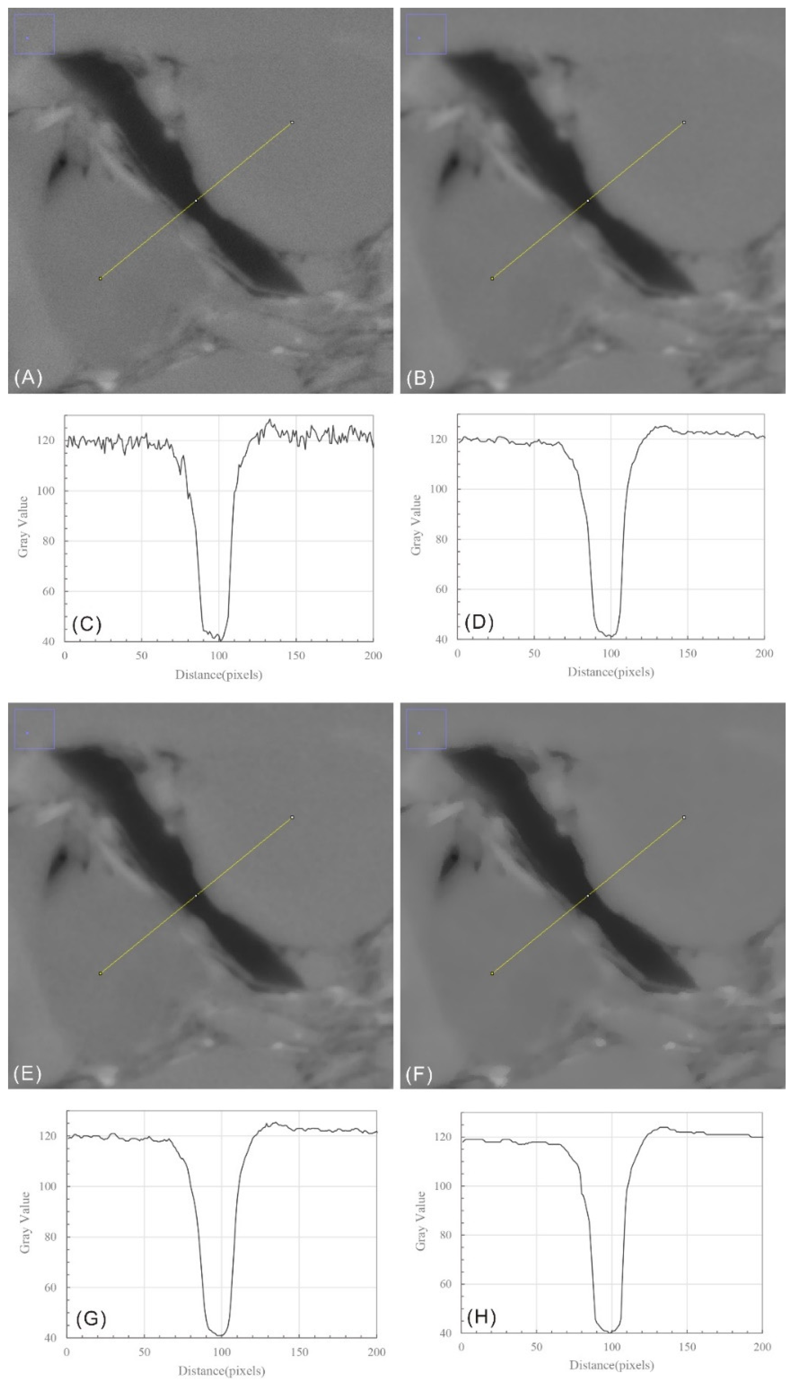
3.1. Image Smoothing

Subject to equipment operating conditions in image signal acquisition processing, as well as external conditions, such as temperature and changing stressors, scanned digital rock images will inevitably generate some noise. Noise influences the analysis of authentic image characterization. Consequently, de-noising is the primary/initial requirement for image smoothing [19]. The more commonly used method for denoising is the digital image filtering method, which mainly includes mean (average) value filtering, median filtering, and Gaussian filtering [20]. More specifically, mean filtering is indicative of a filter template in which the mean grayscale value of each pixel is obtained, whereas median filtering indicates that, within the filter mask, each pixel is assigned a median grayscale value. In Gaussian filtering, however, each point in the center of the filter mask is a target point and the weighting of the remaining points follows the Gaussian distribution, thereby calculating the grayscale value of the target point. In accordance with the corresponding principles, images processed by mean filtering were smoother; however, there was poor processing of image feature boundaries while median filtering had a fixed effect on preserving feature boundary processing. Gaussian filtering was mainly applied to reduce Gaussian noise.
Additionally, smallest univalue segment assimilating nucleus (SUSAN) smoothing (the SUSAN noise filtering algorithm) [21] was also applied in digital rock image smoothing. The principle of SUSAN smoothing is that, within the given filter template range, the threshold is set for the grayscale difference with the target point. A large weight is given to the point where the grayscale difference is within the threshold range, and a small weight is given to points outside the threshold range, so as to effectively preserve the feature boundaries of the image while smoothing the image. Due to the requirements of current mandates, segmentation and identification must be performed on each mineral particle in digital rock images, and retention of border features is required to be relatively high, therefore, median filtering or SUSAN smoothing methods can initially be used. The SUSAN filtration algorithm is presented as follows:
J ( x , y ) = ( i 0 , j 0 I ( x + i , y + j ) × e r 2 2 σ 2 ( I ( x + i , y + j ) I ( x , y ) ) 2 t 2 ) i 0 , j 0 e r 2 2 σ 2 ( I ( x + i , y + j ) I ( x , y ) ) 2 t 2 ,
where (i, j) refers to the pixel position in the filter mask, r = i 2 + j 2 , r indicates the pixel point and the distance from the center pixel, t stands for the brightness margin threshold, σ refers to the Gaussian standard deviation, and i represents the grayscale value of the pixel point.
Smoothing filtering was carried out on the scanned MAPS images. In the image-smoothing process, filters with similar radii were used and different filtering methods (SUSAN, mean, and median) were used on image-smoothing conducted by MAPS. For comparison, smoothing results were obtained for selected replacement areas. More noise signals exist in raw scanned images, resulting in certain changes in the grayscale occurring within the same particle (Figure 1). This will likely influence the grain extraction processes, such as threshold segmentation or grayscale texture. Among each of the filtering methods, mean filtering can make blurred edges, while SUSAN and median filtering retain the edges in images allowing for the realization of a favorable performance. Moreover, after SUSAN filtering, surfaces of particles show comparably increased smoothing. Accordingly, the results of SUSAN smoothing were selected as the basis for correction.

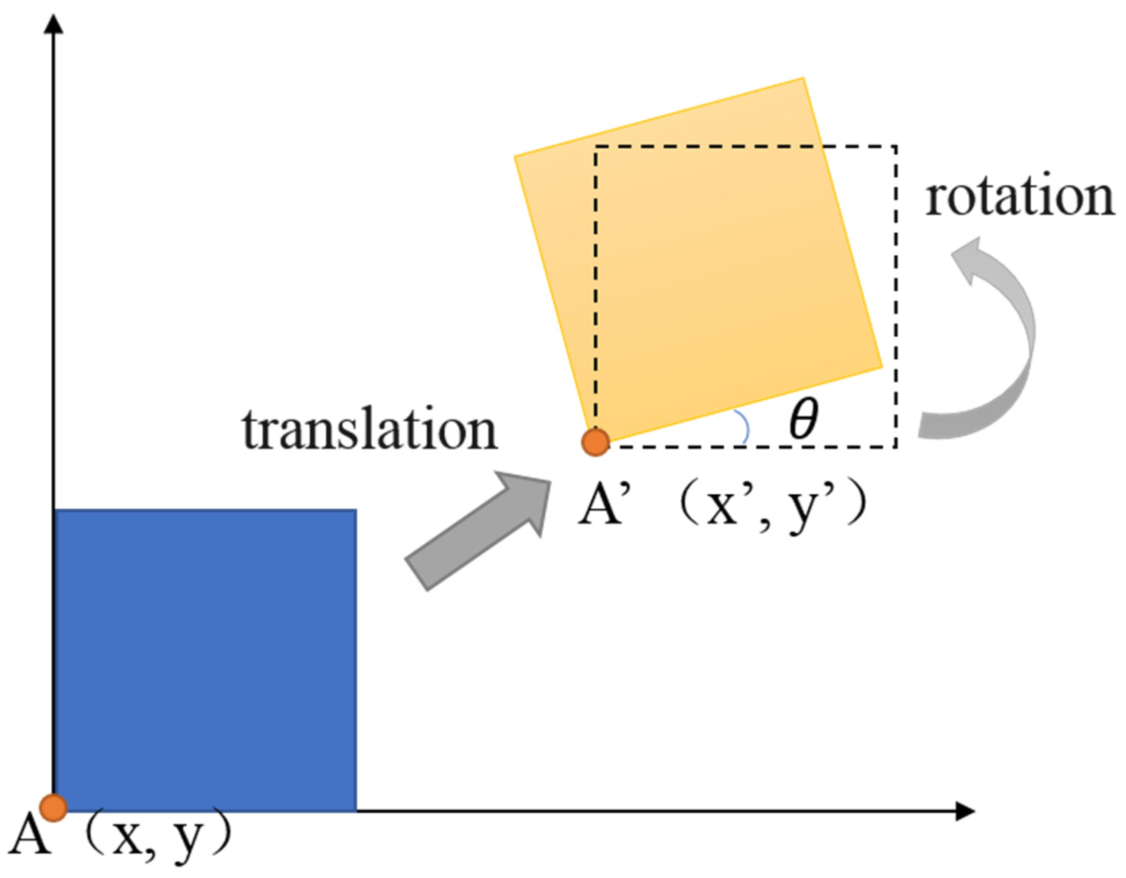
3.2. Image Alignment

Because of the different fields of view and angles during scanning, a given mineral particle can have different positions in QEMSCAN and MAPS images, so the two images cannot be directly used for comparison and correction. Thus, registering and alignment of QEMSCAN and MAPS images are required. The alignment methods are applied to the high-precision backscattering MAPS imagery during mineral quantification analysis of each mineral to carry out calibration and correction.
For QEMSCAN and MAPS images, the differences between the two are mainly translational and rotational, namely, rigid body motion (Figure 2). Therefore, affine transformation can conduct image registration. Generally, parameters related to Equation (2) were selected for point characterization through affine transformation.
{ x = x c o s θ y s i n θ + t x y = y c o s θ + x s i n θ + t y ,
where (x, y) represents the original starting point coordinates, (x′, y′) refers to the point coordinates following affine transformation, (tx, ty) are translation vectors, and θ is the rotation angle.

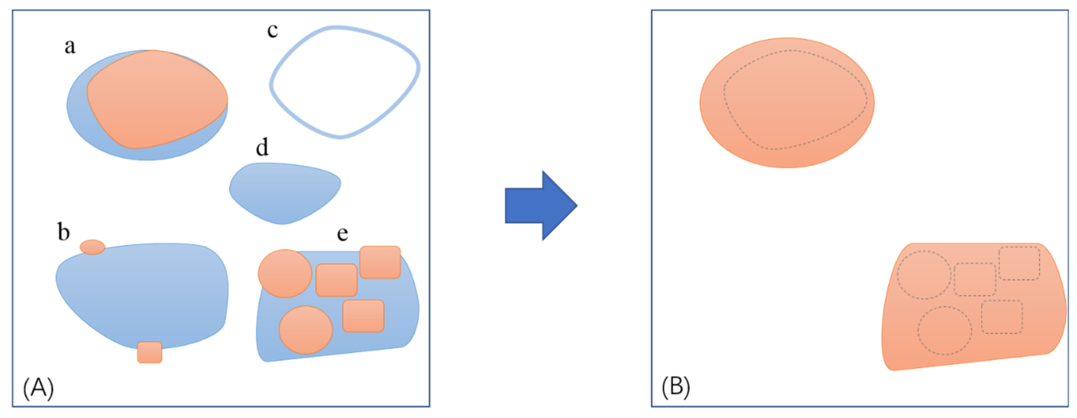
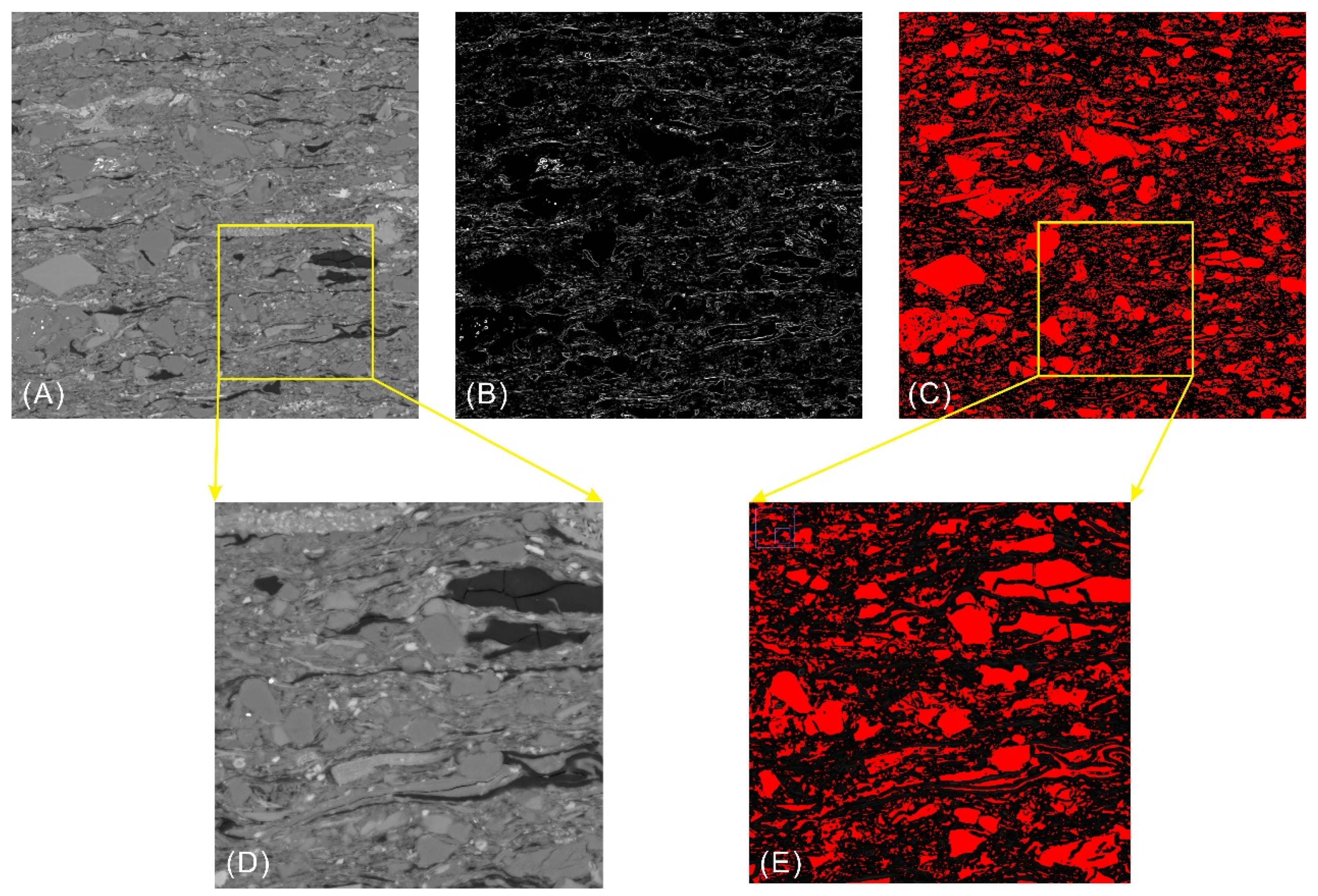
3.3. Mineral Correction
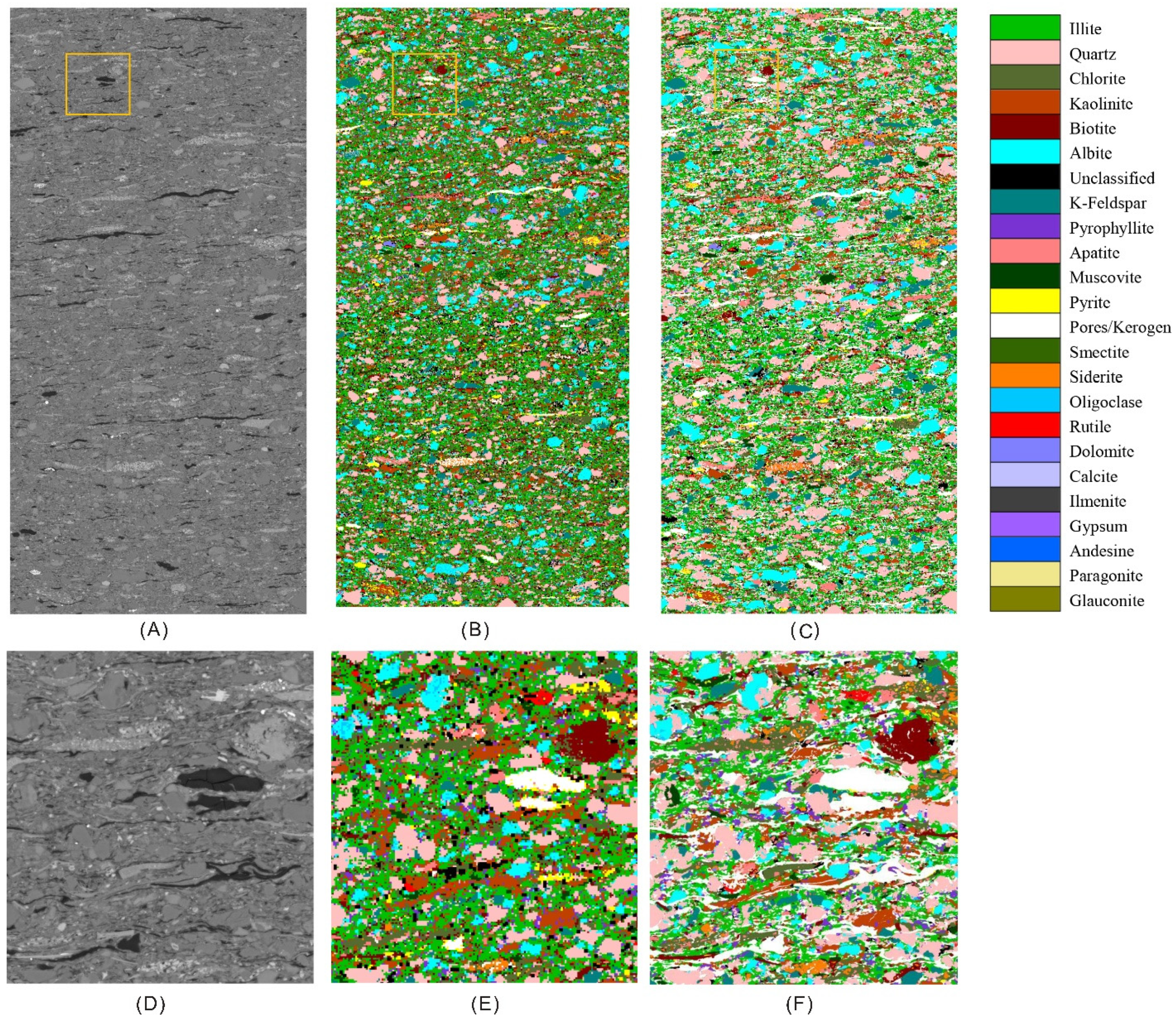
Once QEMSCAN and MAPS images are aligned, MAPS imaging has the capability of conducting feature recognition and correction on various minerals. Owing to the grayscale of MAPS images, the information mainly reflects the density characteristic of each pixel; thereby, the grayscale shade of each point on a MAPS image is reflective of the compositional density. For instance, dark to black areas mainly represent porosity or organic content in rocks, and, in general, porous sections appear lower on the grayscale. Lighter areas mainly represent high-density minerals in rocks, such as pyrite. As a result, greyscale information should provide the best visual determination of mineral type, through which the threshold method can be used for judgment. In addition, because most minerals are composed of some combination of Si, K, Na, Al, and Mg, the middle grayscale range (e.g., 100~200) included numerous mineral types. These minerals can have close grayscale values. Therefore, the grayscale information should be used in combination with other characteristics, such as the grayscale texture of the particular mineral, and the determination of mineral type. Based on this, mineral correction is performed through a combination of these characteristics and QEMSCAN mineral identification results.
According to the aforementioned analyses, the correction of minerals should initially combine QEMSCAN and MAPS images mainly with mineral type data from a grayscale range. Correction should also be inclusive of the distribution of characteristics of various minerals, and comprehensive particle morphology. Specifically, minerals can be classified into the following categories, using different correction methods (Table 1):
Type I: Compositions with distinct grayscale features; threshold segmentation can be directly conducted on MAPS grayscale images to classify components or minerals, such as those having organic material, pores, and pyrite. At the same time, because segmentation along edges typically has one grayscale gradient band, other targets require certain expansion operations after thresholding to restore the objective of determining the actual morphology.
Type II: For minerals with more dispersed particles, better particle contour morphology, small grayscale range, or low grayscale ratio (that is, when the MAPS image is segmented at a threshold, the target mineral will not be segmented together with other minerals, which will result in over-segmentation). These include, but are not limited to, minerals such as apatite, rutile, and siderite. Firstly, the MAPS image can be segmented by grayscale information and multiple target areas with smooth contours and edges can be obtained. Following this, the obtained area and the corresponding area of the mineral on the QEMSCAN image are compared and judged by morphological methods.
The method is described as follows: In Figure 3A, the blue region represents a MAPS image after threshold segmentation into several regions, whereas the orange region represents the target mineral corresponding to the QEMSCAN image. The total surface area S2 of the orange region in a blue region was determined and the proportion of S2 in the surface area S1 of that blue region was calculated. A threshold (th) of that proportion was established (e.g., 80%). If S2/S1 ≥ th, the S1 area was identified as the target mineral and was expanded to a certain degree to obtain relatively realistic mineral particles (regions labeled a and e of Figure 3A). In the other case, the pattern was not associated with the target mineral, such as in regions b and d. For the case of S1, the morphology may be a ringing signal (as seen in region c of Figure 3A). This mainly occurs when threshold segmentation occurring in a selected grayscale range is situated near some particle boundaries causing a grayscale gradient region. For this type of situation, image morphology relationships (e.g., aspect ratio and area/perimeter2) can be used for screening.
Type III: This type relates to minerals with relatively high contents, better particle morphology, more uniform grayscale textures, and easily overlapping minerals through thresholding methods. This includes minerals such as quartz and feldspar. For this type, a certain filter can be built, using the grayscale texture characteristics of the mineral surface to conduct correction. Because the quartz and feldspar mineral components are relatively determinable, the features generally displayed on the grayscale surface of MAPS imagery are more uniform and less noisy. Therefore, extraction can be facilitated by building the simplest variance filters. Through variance filters, uniform grayscale regions and acute changes in grayscale along edges can be effectively extracted. By integrating extracted regions with QEMSCAN images, the determination method can be applied (Figure 3), and this type of mineral can be corrected.
Type IV: A wide grayscale range, relatively no solid morphology, extensive distribution, and comparatively high mineral content, such as clay minerals (e.g., illite, kaolinite), that mainly present as large distributions of patches and more feature outliers on the QEMSCAN images. Due to insufficient resolution, when scanned using QEMSCAN, this type of mineral can be misidentified. For instance, sections with nanoscale porosity or clay pores may be identified as clay minerals, thereby resulting in overestimations of mineral content. Correction of this type of mineral requires first removing the outliers, and then, after correction of the other minerals or components (porosity and organic matter), multiple thresholds and morphological determination methods are needed to restore the real distribution of the minerals.
Type V: For low content, a wide grayscale range or high grayscale ratio, and good particle morphology, outlier pixels on QEMSCAN mineral distribution images are directly filtered out. After obtaining the filtered results, the image can again be amended, for example, through the expansion of particle edges to conduct smoothing.
The specific correction procedure can be carried out according to the difficulty of the mineral correction process. The general order of correction is I−>II−>III−>V−>IV, where correction of clay minerals in Type IV is generally placed last.

4. Results

The above processing steps were performed on the sample. On the basis of image smoothing, the feature points were selected and the MAPS and QEMSCAN images were aligned and cropped by the affine transformation. Following alignment, 12,630 × 25,825 MAPS and QEMSCAN images were obtained. Based on this aligned MAPS image, as well as the observed mineral morphological characteristics, measurements on more than ten major minerals within the main grayscale range in the image were derived. The derived statistics are presented in Figure 4 and Table 2.
The mineral grayscale was mainly within the range of 100~150, in which the peak frequency ratio was 79.5% (Figure 4). The height distribution across the mineral grayscale shows a composition mainly inclusive of illite, kaolinite, albite, montmorillonite, muscovite, K-feldspar, and quartz, among others. All clay minerals also included feldspar, quartz, and other major diagenetic minerals. A large overlap of grayscale values occurs in this region, which, along with high mineral content, prevented direct mineral identification using threshold values. Instead, comprehensive identification required obtaining multiple threshold values and texture characterization. Pyrite, rutile, apatite, and biotite were largely situated in the medium to the high grayscale range; grayscale overlap and mineral content was relatively low, and as such, could be extracted by grayscale and combined with the QEMSCAN image, after which, judgment was made based on morphological comparison methods.
In accordance with the correction order (I−>II−>III−>V−>IV), and the correction methods corresponding to each mineral class, a suitable grayscale range, threshold value for surface morphology, filter ring number, and mineral smoothing were selected. Table 2 shows each identified mineral and its correction. Variance filters identified grayscale textures of quartz and feldspar particles. In addition, a 6 × 6 profile was chosen, and the grayscale variance texture map was obtained. Mineral particles on the texture map were further segmented by threshold values (Figure 5). Notably, for minerals with uniform greyscale textures, such as quartz and feldspar, the particle form extracted by this method was close to the original figure, and some smaller particles could be effectively extracted.
Based on the previously mentioned correction method, the mineral distribution was obtained after the alignment of the QEMSCAN image (Figure 6). The resolution of the mineral distribution map after correction produced a MAPS image with a 25.4 nm resolution, a significant improvement compared to the original QEMSCAN image. In comparison to the original QEMSCAN scanned image, the corrected mineral morphology was overall well-restored (Figure 6). Grain boundaries were noticeable and sharp, and isolated noise in images was noticeably reduced. On this basis, mineral analysis and further research on particle morphology, particle size, particle distribution, and contact relationships can be conducted. It can be seen that the composition of various minerals or components has been corrected to a certain extent (Table 3). In particular, the porosity and organic matter increased from 1.18% before the correction to 17.25%. The concentration of illite was reduced from 30.28 to 26.55%, while chlorite and kaolinite both decreased by about 2%, indicating that the pixels in the QEMSCAN image that were mistakenly divided into clay minerals, due to resolution and other reasons, such as illite, were corrected. Minerals with better particle morphology, such as quartz and feldspar, did not change much before and after correction because the correction mainly restored the mineral boundary morphology and removed the noise on the particles. In addition, the number of unclassified pixels on the corrected QEMSCAN image was significantly reduced. In summary, the morphology and content of various minerals were restored as a whole after the correction, providing a basis for further mineral analysis.

5. Discussion

The comparison showed considerable changes in the content of the various minerals or components after correction (Table 3), especially the content of pore/kerogen, which increased from 1.18% (pre-corrected) to 17.25% (corrected); the content of clay minerals, such as illite, increased from 32.19% to 33.35%, while the content of chlorite and kaolinite decreased by about 1.4% each (Table 3). These changes indicate that the pixel points in the QEMSCAN image that were incorrectly determined as clay minerals due to the limited resolution were corrected. The content of other minerals, such as quartz and feldspar, did not change much after correction, because these minerals have stable composition and good grain morphology, which can be better recognized by QEMSCAN. Our correction work mainly restored the boundary morphology of these minerals and removed the noise on the particles. In addition, our established information fusion correction method was able to significantly reduce the number of pixels in the unrecognized part of QEMSCAN, from 4.69% to 2.98% (Table 3). We explored the use of rock pyrolysis and the XRD results of the selected sample for comparative analysis in order to make a more quantitative evaluation of the accuracy of the correction results.

5.1. Kerogen Content vs. TOC

To assess the kerogen content, we estimated the surface porosity of the selected sample on Maps images, based on the grayscale threshold. The pores of the shale sample mainly included clay mineral intercrystalline pores, organic pores/fractures, intergranular pores/fractures, and intragranular pores (Figure 7). The sample had a high clay mineral content with a large number of clay mineral intercrystalline pores, which represented the majority of the total porosity. The sum of surface porosity of the organic pores/fractures and the intergranular pores/fractures was only about 0.3%. Because of the wide range of grayscale variation of pores in clay minerals and the large difference of pore content in different clay minerals, the surface porosity of clay mineral intercrystalline pores needs to be estimated by region.
The surface porosity of different clay minerals was estimated based on the automatic identification of MAPS images in combination with previous research results [22]. The surface porosity of illite, chlorite, and kaolinite are about 20%, 10%, and 10%, respectively. Therefore, the equation for calculating the surface porosity of the samples is simplified as:
2 D = i = 1 n C i × i + o t h e r s
where 2 D is the surface porosity of the whole sample, C i   and   i are the 2D area share of clay minerals (illite, chlorite, and kaolinite) and their porosity, respectively, and o t h e r s is the 2D area share of non-clay pores, such as organic pores and intergranular pores.
The calculation yields a surface porosity of about 6.86% for the whole sample. According to the area ratio of pore/kerogen (Table 3), the surface content of kerogen C k e r o g e n can be deduced to be about 10.56%. Considering the thermal maturity [23] and the type of kerogen, the kerogen density of the sample was about 1.3 g/cm3 [24]. The density of the shale sample was 2.3 g/cm3. Therefore, we calculated the kerogen content of the sample to be about 6.26 wt.%, using the following equation.
T O C = C k e r o g e n × γ C k e r o g e n × γ + ( 1 C k e r o g e n ) × ρ b 100 %
where TOC is the total organic carbon content, %; C k e r o g e n is the kerogen surface content, %, γ is the kerogen density, g/cm3, and ρ b is the shale density, g/cm3.
This result is close to the TOC value of 7.49 wt.% measured by rock pyrolysis (See supplementary Material Table S1). Based on QEMSCAN results, following the above equations and steps, the calculated TOC content was negative, which is unreasonable. Therefore, the results of the image correction are reliable, and the accuracy evaluation of pore/kerogen further supports the importance and rationality of image correction.

5.2. Major Minerals Content vs. XRD

We removed pore/kerogen and unclassified components from the corrected results, and then compared the identified mineral content results after normalizing with the XRD test results (Table 3). For comparison under the same unit system, the mineral mass percentage results measured by XRD were converted to volume percentage with the following equation:
v o l i = w i / ρ i i = 1 n w i / ρ i × 100
where v o l i is the mineral volume percentage, vol.%, w i is the mineral mass percentage, wt.%, and ρ i is the mineral density, g/cm3. Note that the content of the illite–smectite mixed-layer (I/Smix) was calculated according to the mixed layer ratio I/S (%S) with the following equation:
ρ I / S = I / S 1 + I / S × ρ Illite + 1 1 + I / S × ρ Smectite
where ρ I / S is the density of the illite-smectite mixed-layer, g/cm3, I / S is the mixed layer ratio, a decimal with value of 0.1, ρ Illite is the illite density, g/cm3, and ρ Smectite is the smectite density, g/cm3.
Since QEMSCAN identifies more mineral species than XRD, we simplified the QEMSCAN results, including classifying mica as clay minerals and combining illite and smectite. Image correction did not result in significant changes in the major mineral contents. Overall, the clay mineral and non-clay mineral contents identified by the QEMSCAN technique were comparable to the XRD results. Because of heterogeneity, from 2D to 3D, there must be a difference between the mineral content identified by the image and that measured by X-ray diffraction. For example, for quartz content, the QEMSCAN, corrected and XRD results were 18.31%, 21.63% and 31.09%, respectively (Table 3). For clay minerals, QEMSCAN can effectively identify mixed-layer clay minerals. Considering the uncertainties in identification and possible error determination on the illite–smectite mixed-layer and illite mineral in the interpretation process, the composition and content of clay minerals identified by QEMSCAN were similar to XRD, and the corrected clay mineral content was significantly closer to the XRD results. Reducing the error caused by dimension switching is an important research point in the future.
According to the above analysis, the shale mineral analysis method fully combines the advantages of the most advanced mineral quantitative analyses, QEMSCAN technology, and high-resolution large-scale backscatter scanning electron microscopy analysis technology, and corrects the quantitative analysis results of QEMSCAN minerals using image smoothing, image alignment, image segmentation, and morphological analysis, and obtains the high-precision 2D quantitative distribution of shale minerals. In particular, it can effectively correct the content of clay minerals, pores, and organic matter components, and restore particle morphology and boundaries, among other parameters. This approach overcomes the shortcomings of conventional shale mineral analysis methods and shows obvious advantages. Based on the high-precision mineral distribution obtained by this method, its application can be further expanded, such as for counting the particle size distribution of various minerals, analyzing the distribution trends of organic matter or pores, and using random modeling methods to establish a 3D distribution model of shale minerals. This can further provide support for comprehensive shale reservoir evaluation, prospective zone prediction, fracturing transformation, and other shale-related evaluations.
At present, the use of this method has only been carried out in preliminary exploration and research work. The classification of minerals (that is, the selection of correction methods), and the selection of correction parameters, are affected by human subjectivity, actual mineral distribution characteristics, and other factors. Furthermore, there is no unified set of division standards and correction methods. Some minerals in scanned QEMSCAN samples may need to combine the actual morphological characteristics and distribution characteristics of minerals with other parameters. In this study, a variety of methods were selected for comprehensive correction to obtain a better correction effect. Therefore, for the shale mineral analysis method, the next step should be to further optimize the image-processing methods. This will include improving mineral classification and morphological correction, adaptability, and automation, and increasing the accuracy of the correction results of the method. This could further extend to the use of current cutting-edge machine learning, deep learning, and other artificial intelligence analysis methods to establish mineral correction and recognition models. In this way, the automatic correction and analysis evaluation of shale minerals based on QEMSCAN images and MAPS images can be used to establish a more effective, reasonable, and widely applicable shale mineral analysis method.

6. Conclusions

A shale mineral analysis method, based on quantitative mineral analysis (QEMSCAN) and high-resolution large-scale backscatter scanning electron microscopy (MAPS), was developed. This method makes full use of the 2D mineral distribution of QEMSCAN images and the high-resolution advantages of MAPS scanning electron microscopy images. By using techniques such as image smoothing, image alignment, image segmentation, and morphological analysis, the results of quantitative analysis of QEMSCAN minerals were corrected. An analysis of Ordos Basin shale samples showed that this method can reduce the noise of mineral distribution images, and effectively correct the content of various minerals and components, such as clay minerals and pores/organic matter in shale. In addition, this method can restore the morphology and contours of mineral particles (such as quartz and feldspar), and, thereby, obtain a high-precision 2D quantitative distribution of shale minerals, providing a basis for further mineral analysis and application. This method lays a foundation for further optimization of image-processing methods, such as mineral classification, texture extraction, and morphological correction. In the future, the expectation is to explore the use of artificial intelligence technologies, such as deep learning, to study the inherent characteristics of mineral forms, establish mineral correction and identification models, and realize automatic mineralogical analysis and evaluation.

Supplementary Materials

The following supporting information can be downloaded at: https://www.mdpi.com/article/10.3390/app12105013/s1, Table S1: TOC and Rock-Eval results of the shale sample.

Author Contributions

Conceptualization, S.L.; methodology, S.L.; software, S.L. and L.H.; formal analysis, S.L.; resources, X.L.; writing, S.L.; visualization, S.L.; supervision, L.H.; project administration, L.H.; funding acquisition, L.H. All authors have read and agreed to the published version of the manuscript.

Funding

This study was funded by the China National Petroleum Corporation (CNPC) Science and Technology Development Project (No. 2021DJ5202).

Institutional Review Board Statement

Not applicable.

Informed Consent Statement

Not applicable.

Data Availability Statement

Not applicable.

Conflicts of Interest

The authors declare no conflict of interest.

References

  1. Madi, J.A.; Belhadj, E.M. Unconventional Shale Play in Oman: Preliminary Assessment of the Shale Oil/Shale Gas Potential of the Silurian Hot Shale of the Southern Rub al-Khali Basin. In Proceedings of the SPE Middle East Unconventional Resources Conference and Exhibition, Muscat, Sultanate of Oman, 26–28 January 2015. [Google Scholar]
  2. Adiguna, H.; Torres-Verdín, C. Comparative Study for the Interpretation of Mineral Concentrations, Total Porosity and TOC in Hydrocarbon-Bearing Shale from Conventional Well Logs. In Proceedings of the SPE Annual Technical Conference and Exhibition (SPE-166139-MS), New Orleans, LA, USA, 30 September 2013. [Google Scholar]
  3. Desaki, S.; Kobayashi, Y.; Asaka, M. The effect of mineral properties on rock physics modeling of shale anisotropy. In Proceedings of the SEG International Exposition and Annual Meeting (SEG-2019-3214237), San Antonio, TX, USA, 15 September 2019. [Google Scholar]
  4. Wanniarachchi, W.; Ranjith, P.G.; Perera, M.; Nguyen, J.T.; Rathnaweera, T.D. An Experimental Study to Investigate the Effect of Mineral Composition on Mechanical Properties of Shale Gas Formations. In Proceedings of the 51st US Rock Mechanics/Geomechanics Symposium (ARMA-2017-0433), Richardson, TX, USA, 25–28 June 2017. [Google Scholar]
  5. Fakhry, A.; Hoffman, T. The Effect of Mineral Composition on Shale Oil Recovery. In Proceedings of the Unconventional Resources Technology Conference (URTEC-2902921-MS), Houston, TX, USA, 23–25 July 2018. [Google Scholar]
  6. Al Ismail, M.; Zoback, M. CO2-Based Technologies in Unconventional Resources: Impact of Rock Mineralogy on Adsorption. In Proceedings of the SPE Kingdom of Saudi Arabia Annual Technical Symposium and Exhibition (SPE-188168-MS), Dammam, Saudi Arabia, 24 April 2017. [Google Scholar]
  7. Gies, R.M. An Improved Method for Viewing Micropore Systems in Rocks with the Polarizing Microscope. SPE-13136-PA. SPE Form. Eval. 1987, 2, 209–214. [Google Scholar] [CrossRef]
  8. Thornley, D.M. Thermogravimetry/evolved water analysis (TG/EWA) combined with XRD for improved quantitative whole-rock analysis of clay minerals in sandstones. Clay Miner. 1995, 30, 27–38. [Google Scholar] [CrossRef]
  9. Kamruzzaman, A. Petrophysical Rock Typing of Unconventional Shale Plays: A Case Study for the Niobrara Formation of the Denver-Julesburg (DJ) Basin; Colorado School of Mines: ProQuest Dissertations Publishing: Ann Arbor, MI, USA, 2015. [Google Scholar]
  10. Faisal, T.F.; Awedalkarim, A.; Chevalier, S.; Jouini, M.S.; Sassi, M. Direct scale comparison of numerical linear elastic moduli with acoustic experiments for carbonate rock X-ray CT scanned at multiresolutions. J. Pet. Sci. Eng. 2017, 152, 653–663. [Google Scholar] [CrossRef]
  11. Julie, J.K.; Florence, T.L.; Dan, A.P.; Andres, F.C.; Antonio, L.; Matthew, N.; Catherine, A.P. SMART mineral mapping: Synchrotron-based machine learning approach for 2D characterization with coupled micro XRF-XRD. Comput. Geosci. 2021, 156, 104898. [Google Scholar]
  12. Maqsood, A.; Manouchehr, H. Mineralogy and Petrophysical Evaluation of Roseneath and Murteree Shale Formations, Cooper Basin, Australia Using QEMSCAN and CT-Scanning. In Proceedings of the SPE Asia Pacific Oil and Gas Conference and Exhibition (SPE-158461-MS), Perth, Australia, 22 October 2012. [Google Scholar]
  13. Fialips, C.I.; Labeyrie, B.; Burg, V.; Mazière, V.; Jacquelin-Vallée, L. Quantitative Mineralogy of Vaca Muerta and Alum Shales From Core Chips and Drill Cuttings by Calibrated SEM-EDS Mineralogical Mapping. In Proceedings of the Unconventional Resources Technology Conference (URTEC-2902304-MS), Houston, TX, USA, 23–25 July 2018. [Google Scholar]
  14. Hofmann, A.; Rigollet, C.; Portier, E.; Burns, S. Gas Shale Characterization-Results of the Mineralogical, Lithological and Geochemical Analysis of Cuttings Samples from Radioactive Silurian Shales of a Palaeozoic Basin, SW Algeria. In Proceedings of the North Africa Technical Conference and Exhibition (SPE-164695-MS), Cairo, Egypt, 15 April 2013. [Google Scholar]
  15. Goergen, E.T.; Curtis, M.; Jernigen, J.; Sondergeld, C.; Rai, C. Integrated Petrophysical Properties and Multi-Scaled SEM Microstructural Characterization. In Proceedings of the SPE/AAPG/SEG Unconventional Resources Technology Conference (URTEC-1922739-MS), Denver, CO, USA, 25 August 2014. [Google Scholar]
  16. Lemmens, H.; Goergen, E.; Skinner, K.; Owen, M. From SEM Maps and EDS Maps to Numbers in Unconventional Reservoirs. In Proceedings of the SPE/AAPG/SEG Unconventional Resources Technology Conference (URTEC-1581248-MS), Denver, CO, USA, 12–14 August 2013. [Google Scholar]
  17. Barker, C. Pyrolysis techniques for source-rock evaluation. Am. Assoc. Pet. Geol. Bull. 1974, 58, 2349–2361. [Google Scholar]
  18. Peters, K. Guidelines for evaluating petroleum source rock using programmed pyrolysis. Am. Assoc. Pet. Geol. Bull. 1986, 70, 318–329. [Google Scholar]
  19. Ebadi, M.; Makhotin, I.; Orlov, D.; Koroteev, D. Digital Rock Physics in Low-Permeable Sandstone, Downsampling for Unresolved Sub-Micron Porosity Estimation. In Proceedings of the SPE Europec (SPE-200595-MS), Virtual, 1 December 2020. [Google Scholar]
  20. Diwakar, M.; Kumar, M. A review on CT image noise and its denoising. Biomed. Signal Process. Control 2018, 42, 73–88. [Google Scholar] [CrossRef]
  21. Smith, S.M.; Brady, J.M. SUSAN—A new approach to low level image processing. Int. J. Comput. Vis. 1997, 23, 45–78. [Google Scholar] [CrossRef]
  22. Guillaume, D.; Janos, L.U.; Peter, A.K.; Jan, K.; Claudia, B. High-resolution 3D fabric and porosity model in a tight gas sandstone reservoir: A new approach to investigate microstructures from mm-to nm-scale combining argon beam cross-sectioning and SEM imaging. J. Pet. Sci. Eng. 2011, 78, 243–257. [Google Scholar]
  23. Okiongbo, K.S.; Aplin, A.C.; Larter, S.R. Changes in type II kerogen density as a function of maturity: Evidence from the Kimmeridge Clay Formation. Energy Fuels 2005, 19, 2495–2499. [Google Scholar] [CrossRef]
  24. Wu, Z.; Xu, Z. Experimental and molecular dynamics investigation on the pyrolysis mechanism of Chang 7 type-II oil shale kerogen. J. Pet. Sci. Eng. 2022, 209, 109878. [Google Scholar] [CrossRef]
Figure 1. Results of different smoothing methods compared with the original images. (A) The original image. (B) The image processed with mean filter smoothing. (C) The grayscale values at different pixel locations of the yellow line in Figure 1 (A). (D) The grayscale values at different pixel locations of the yellow line in Figure 1 (B). (E) The image processed with median filter smoothing. (F) The image processed with SUSAN smoothing. (G) The grayscale values at different pixel locations of the yellow line in Figure 1 (E). (H) The grayscale values at different pixel locations of the yellow line in Figure 1 (F).
Applsci 12 05013 g001
Figure 2. Schematic diagram showing affine transformation on a solid object.
Applsci 12 05013 g002
Figure 3. Schematic diagram showing the identification of Type B minerals. (A) Segmentation at the threshold value of the MAPS image after superposition of the associated QEMSCAN on the targeted mineral distribution map. (B) The mineral distribution after correction. Blue refers to the results of the MAPS threshold segmentation, while yellow represents the QEMSCAN mineral distribution.
Applsci 12 05013 g003
Figure 4. MAPS image grayscale frequency distribution map, the grayscale range, and content of each major mineral.
Applsci 12 05013 g004
Figure 5. Illustration of the effect of the 6 × 6 variance filter template for extracting homogeneous mineral particles, in which (A) is the original image, (B) is the textured grayscale variance image, and (C) is the image extracted from threshold values for the textured grayscale variance, (D) is a partial enlargement of Figure 5A (yellow box). (E) is a partial enlargement of Figure 5C (yellow box).
Applsci 12 05013 g005
Figure 6. Aligned MAPS image (A) with QEMSCAN image (B) and an image of the corrected mineral distribution (C). The correction effect is shown in detail, (DF) correspond to the yellow box area of the respective images in Figure 6 (AC).
Applsci 12 05013 g006
Figure 7. Main pore/fracture types of the shale sample.
Applsci 12 05013 g007
Table 1. Summary of the mineral types and correction methods.
TypeCharacteristicsMethodRepresentative Minerals and Components
Obvious grayscale featuresMAPS image threshold segmentation + particle expansionOrganic matter, pores, pyrite
Relatively dispersed particles; good particle profile morphology; minimal overlap with other minerals during thresholdingMAPS image threshold segmentation + morphology + particle expansionApatite, rutile, siderite
High component content; good profile morphology; uniform grayscale texture; easy overlap with other minerals during thresholdingVariance and other texture feature extraction + morphology + particle expansionQuartz; feldspar
Wide grayscale range; no solid morphology; wide distribution; high component/mineral content1. QEMSCAN image outlier filteringIllite, kaolinite
2. Multiple thresholds + morphology
Low mineral content; wide grayscale range or high grayscale ratio; good particle morphology1. QEMSCAN image outlier filteringDolomite, calcite
2. Particle expansion
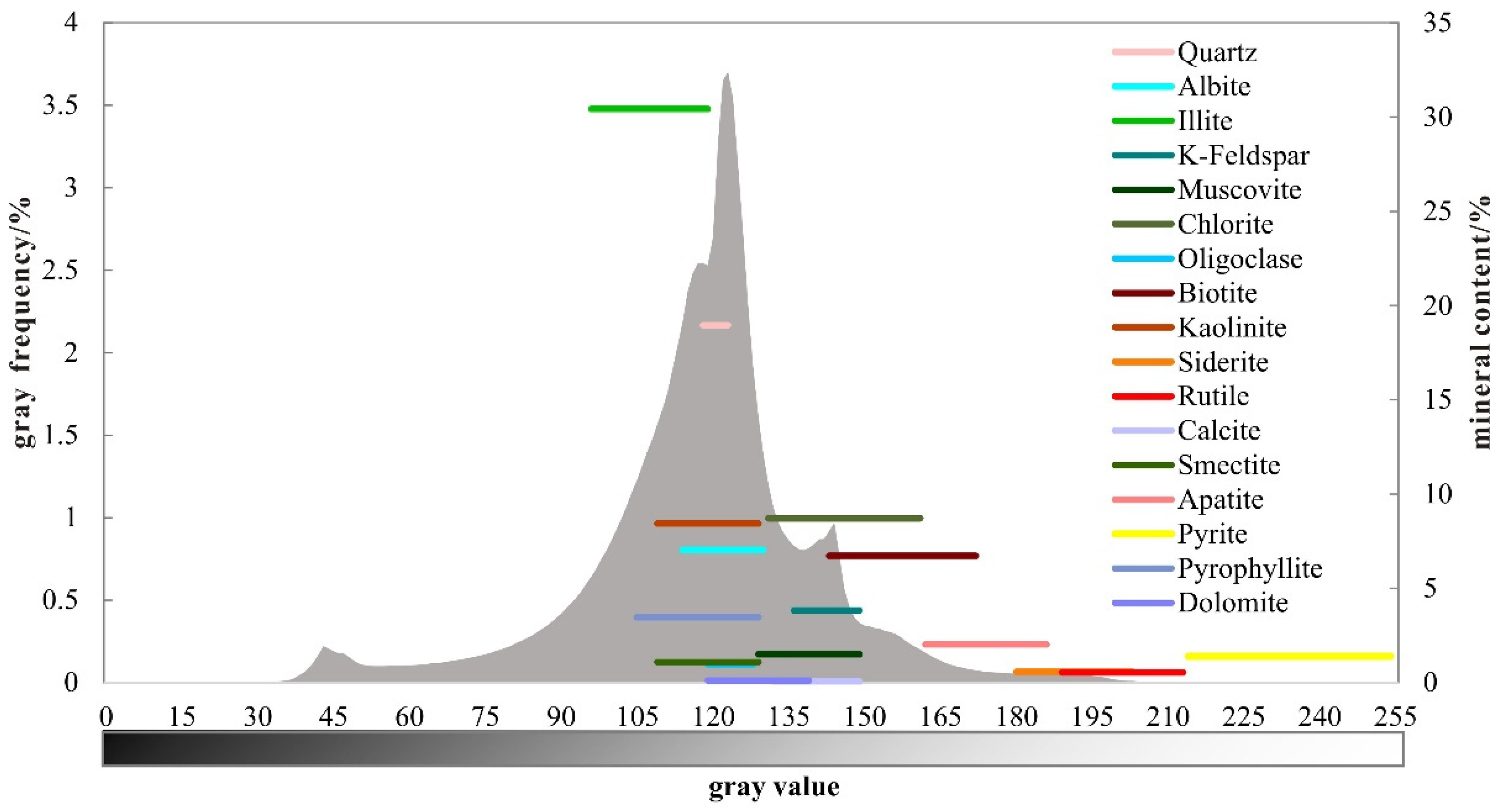
Table 2. The grayscale range, content, and classification of each major mineral and component.
MineralGrayscale Value RangeContent (%)Classification
Minimum Grayscale ValueMaximum Grayscale Value
Pyrite2152551.39
Pores/Kerogen0960.89
K-Feldspar1371503.82
Muscovite1301501.5
Biotite1441736.72
Siderite1812040.57
Rutile1902140.53
Apatite1631872.02
Quartz11912418.95
Albite1151317.03
Illite9712030.42
Chlorite1321628.71
Kaolinite1101308.43
Smectite1101301.08
Pyrophyllite1061303.46
Dolomite1201400.11
Oligoclase1201290.97
Calcite1331500.06
Table 3. Comparison among the mineral/component surface content values by QEMSCAN-MAPS correction and volume content values by XRD.
Mineral/ComponentContent by QEMSCAN (%)Corrected Content (%)XRD (vol.%)XRD (wt.%)Density (g/cm3)
Pores/Kerogen1.1817.22//
Unclassified4.692.98//
Non-clay minerals *Quartz18.3121.6331.0930.8
K-Feldspar4.415.239.79.92.57
Albite6.928.968.498.62.63
Pyrite1.651.040.621.25.00
Clay mineralsBiotite8.015.25//
Muscovite1.831.58//
Illite32.1933.359.8110.42.75
Kaolinite8.967.566.376.442.62
Chlorite9.358.17.538.422.90
Smectite1.240.29//2.35
I/Smix//26.3824.262.39
Total **Non-Clay38.4243.8649.9
Clay61.5856.1450.1
* Due to low content and non-detection by XRD, some non-clay minerals of QEMSCAN are not listed here, including pyrophyllite, apatite, siderite, oligoclase, rutile, dolomite, and calcite. ** The content results of identified minerals are normalized to 100 percent, after pore/kerogen and unclassified components are removed.
Publisher’s Note: MDPI stays neutral with regard to jurisdictional claims in published maps and institutional affiliations.

