Abstract
Visualization of soft tissues in microCT scanning using X-rays is still a complicated matter. There is no simple tool or methodology on how to set up an optimal look-up-table while respecting the type of soft tissue. A partial solution may be the use of a contrast agent. However, this must be accompanied by an appropriate look-up-table setting that respects the relationship between the soft tissue type and the Hounsfield units. The main aim of the study is to determine experimentally derived look-up-tables and relevant values of the Hounsfield units based on the statistical correlation analysis. These values were obtained from the liver and kidneys of 24 mice in solutions of ethanol as the centroid value of the opacity look-up-table area under this graph. Samples and phantom were scanned by a Bruker SkyScan 1275 micro-CT and Phywe XR 4.0 and processed using CTvox and ORS Dragonfly software. To reconstruct the micro-CT projections, NRecon software was used. The main finding of the study is that there is a statistically significant relationship between the centroid of the area under the look-up-table curve and the number of days for which the animal sample was stored in an ethanol solution. H1 of the first hypothesis, i.e. that suggested the Spearman’s correlation coefficient does not equal zero (r1 ≠ 0) regarding this relationship was confirmed. On the other hand, there is no statistically significant relationship between the centroid of the area under the look-up-table curve and the concentration of the ethanol solution. In this case, H1 of the second hypothesis, i.e. that the Spearman’s correlation coefficient does not equal zero (r2 ≠ 0) regarding this relationship was not confirmed. Spearman’s correlation coefficients were −0.27 for the concentration and −0.87 for the number of days stored in ethanol solution in the case of the livers of 13 mice and 0.06 for the concentration and 0.94 for the number of days stored in ethanol solution in the case of kidneys of 11 mice.
Keywords:
micro-CT; transfer function; look-up-table; soft tissue; CT number; Hounsfield unit; visualization 1. Introduction
Computed tomography (CT) imaging is widely used in medical practice, mainly due to the non-invasiveness of this method, its good spatial resolution, and the relatively short acquisition time of the required images. In addition to conventional CT, which is mainly used both for diagnostic and therapeutic procedures [1], high spatial resolution CT or micro-CT (μCT) are also used in practice [2]. These systems work on the same basic principle as the typical CT, except that the X-ray-tube-detector system does not perform rotational motion, but rotates the specimen. However, their advantage lies in their ability to scan samples with much higher spatial (<50 μm) and contrast resolution.
It is because of the non-destructiveness of this method in evaluating the scanned volume with high resolution that µCT devices are much used in both research and industry. Furthermore, even if the intrinsic noise of commercial µCT detectors is not a problem in many cases (especially in industry), the imaging of more delicate structures with a lower range of CT numbers (the same as Hounsfield units = HU), and the associated lower attenuation contrast between structures, such as soft tissues, is greatly hampered by this noise.
The present work, in collaboration with the Department of Anatomy at the 3rd Faculty of Medicine, Charles University (Prague, Czech Republic), is primarily focused on the visualization of soft tissues in particular, as well as the search for a methodology that could optimize the overall visualization process and make it easier. This also involves research and experimentation with new procedures and contrast agents to achieve the required contrast between soft tissues that is needed for visualization [3,4,5,6,7].
Two papers dealt with similar issues. The first one, i.e., [8], used an image histogram for optimal look-up-table (LUT) setup. Thus, it is not the same intention. The second work, i.e., [9], uses only the LUT settings. However, in neither case was it possible to find a link between soft tissue type and Hounsfield units.
We have been using μCT for a long time and we need to visualize soft tissues in experimental animals. For a long time, there is a tradition of contrast agent usage, but they are not always best and/or we often encounter problems when using them. This is why we tried to figure out some connection between LUT setting and HU values for individual structures and organs; even mentioned contrast agents could have been of some value in this. Additionally, we wanted to find out if there exist other possibilities of contrast enhancement, e.g., because of air bubbles in contrast agent for ultrasound. Especially this is considered when experimenting with PHYWE XR 4.0 in various structures in chicken tissues (phantom). Finally, we also think about semiautomated, or fully automated settings of LUT with fuzzy logic. Some of these ideas were verified within this study.
The main aim of this study is to optimize soft tissue contrast visualization of biological specimens (mouse liver, kidneys) using a contrast agent and a proper LUT. Based on this aim we would like to statistically verify the relationship between the centroid of the area under the look-up-table curve and the number of days for which the animal sample was stored in the ethanol solution, as well as the concentration of the ethanol solution. Therefore, two hypotheses were formulated. H1 (Each occurrence of H1 means that it is an allernative hypothesis) of the first hypothesis states that the Spearman’s correlation coefficient does not equal zero (r1 ≠ 0) in the case of relationship between the coordinates of the center of gravity (centroid) of the area under the LUT and the number of days for which the sample was stored in the ethanol solution. H1 of the second hypothesis states that the Spearman’s correlation coefficient does not equal zero (r2 ≠ 0) in the case of relationship between the coordinates of the center of gravity (centroid) of the area under the LUT and the ethanol concentration in the solution.
2. Materials and Methods
2.1. Materials, Devices, and Software
The database of µCT images from the Dept. of Anatomy of the 3rd Medical Faculty of Charles University was used for the study.
All intravenous contrast agent’s applications follow similar pattern. At first there is introduced the contrast agent into the tail vein. After that follows animal euthanasia and µCT scanning. Concerning Aurovist contrast agent, solution from the ampoule is injected into tail vein under isoflurane anesthesia into the bloodstream. Follows scanning in the µCT apparatus. Concerning the timing, scanning is performed after complete distribution of Aurovist gold nanoparticles to the tissues of the animal, including both arteries and veins of the circulatory system.
Preparation steps for experimental animals were the following.
Animals (mice) were housed in the standard light/dark cycle in the First Faculty of Medicine, Charles University at standard room temperature. Mice were applied one ampulla of Aurovist contrast agent (15 nm of Aurum particles in 40 mg of solution, Nanoprobes, Yaphank, NY, USA) in the tail vein per one mouse. In case of whole mouse experiment, 2 h after Aurovist application were mice euthanized with pentobarbital and scanned in micro-CT. Timing was selected because rigor mortis develops within 2 h after death.
Animals (chickens) were obtained by micro-surgery from the eggs in their 19 days of development. Firstly, a rectangular window was dissected out of the egg wall and solution of 40% KI to euthanize chicken (heartbeat stop) was applied intra-amniotically. After the removal of dead chicken from the egg it was placed into 80% of Ethanol for 7 days.
Animals (rabbits) were donated by Prof. Berndt Minnich, University of Salzburg, Vascular Unit, Austria. Post-mortem, rabbits were pinned in supine position onto a wax plate. After opening of the abdomen, the aorta abdominalis was identified and separated from each other. A ligature around the aorta abdominalis ensured exclusive upper body casting. A tube was inserted into the artery cranially to the first ligature and tied in place (6.0 sutures). Blood vessels were rinsed after opening the aorta with 0.9% Ringer’s solution (60 mL/h) at 37 °C until clear reflux appeared. Thereafter, the casting medium (Mercox-Cl-2B, Ladd Research Inc., Burlington, VT, USA) diluted with monomeric methyl methacrylate was injected at 99 mL/h by an electric syringe pump (Habel PSA 50, Sky Electronics S.A., Grenoble, France) or a pneumatic injection pump (ComServ OG, Ebenau, Austria). When the injected resin became viscous, animals were left in place for at least 30 min at room temperature (RT) to initiate resin polymerization. The upper bodies of the rabbits were cut off and tempered in water (60 °C, 24 h). Subsequently, water was replaced by potassium hydroxide (7.5%, 40 °C, twice for 24 h), followed by hydrochloric acid (2%, RT, 24 h) and formic acid (5%, RT, 15 min). Finally, casts were washed thrice and frozen in distilled water (−20 °C) and freeze-dried (FreeZone 77520, Labconco Corp., Kansas City, MO, USA).
The database consisted of ex vivo chickens in and out of the shell and aged 5 to 19 days. Chickens outside the shell were preserved in 50–100% ethanol solution, some of them additionally in formaldehyde solution. In addition, a few chicken samples contained injected gold nanoparticles from the Aurovist contrast agent. Prior to acquisition, samples were left in air after removal from the solution and scanned with Bruker’s SkyScan 1275 (Bruker MicroCT, Kontich, Belgium) after evaporation of the solution.
Another part of the database consisted of ex vivo preparations of mice injected with Aurovist contrast agent containing 15 nm gold nanoparticles (AuNPs) prior to scanning.
A 50% solution of Omnipaque contrast agent was then used intravenously before scanning the mouse organs themselves (liver, lungs, spleen, and heart).
Some mouse organs, such as liver, kidney, brain, heart, and leg, were kept for one week in a solution of potassium iodide with concentration 100 mM (KI, Merck, Czech Republic) in 20% ethanol before scanning.
Lastly, the database included corrosive preparations in which a resin (Mercox) [10] was infused into the vascular system and allowed to harden, the remaining tissue was then dissolved in lye by maceration and the sample was scanned. Corrosive preparations of rabbit and rat lung and heart were selected for the purpose of this study.
For the implementation of the idea of blood vessels visualization in soft tissue using the contrast that would be created by the presence of air in the vascular cavities, chicken flesh was used as a phantom in which cylindrical tubes/capillaries of various diameters made of different materials were placed. These were two tubes (silicone), a glass capillary with sealed ends, and a plastic straw (bioplastic PLA). This phantom, depicted in Figure 1, was then scanned with the Phywe XR 4.0 (PHYWE Systeme GmbH & Co. KG, Göttingen, Germany) experimental setup.
Figure 1.
Chicken sample with capillaries as vascular phantom (top) and phantom X-ray image (bottom); materials from left: bioplastic PLA, glass, green silicone, and transparent silicone. Scale is in [cm].
Two µCT systems were used to scan the above samples. The ex vivo chicken samples were scanned with a professional µCT system Bruker SkyScan 1275 located at the Department of Anatomy, 3rd Faculty of Medicine, Charles University, while the Phywe XR 4.0 experimental setup was used to scan the phantom of the chicken vasculature and capillaries at the Dept. of Biomedical Technology, Fac. of Biomedical Engineering, Czech Technical University in Prague.
Bruker’s SkyScan 1275 has been specifically designed for fast scanning using advances in X-ray source technology and efficient flat-panel detectors. This X-ray source has the selectable anode voltage of the assembly ranging from 20 to 100 kV and the max. available power is 10 W. The assembly includes an active 3 megapixel CMOS flat-panel detector with a maximum possible resolution of up to 4 μm (at maximum magnification) and it is capable of accommodating a sample diameter of 96 mm and a height of 120 mm. All used setups of the above mentioned µCT are available within the Appendix B, i.e., Table A2, Table A3, Table A4, Table A5, Table A6, Table A7, Table A8, Table A9, Table A10, Table A11, Table A12, Table A13, Table A14, Table A15, Table A16, Table A17, Table A18 and Table A19.
The XR 4.0 experimental setup from the German company Phywe was designed for teaching purposes and for laboratory experiments with X-rays. Its advantage lies, among other things, in the relatively easy and quick interchangeability of the X-ray tube and, therefore, facilitates experiments with different anode materials [11,12].
The XR 4.0 can also be used as a µCT system thanks to an expansion kit supporting the computed tomography function. This set consists of a fixed copper X-ray tube that illuminates the specimen on a rotary table driven by a stepper motor with a minimum adjustable table rotation angle of 0.086°. The attenuated X-ray radiation is then incident on an XRIS detector (CMOS) with an active area of 5 × 5 cm2 and a maximum possible resolution of 48 μm [11,12]. The selectable anode voltage of the assembly is 5–35 kV with an adjustable emission current in the range up to 1 mA. Setup with detailed setting is available within the Appendix B, i.e., Table A1.
As regards the software, CTvox (Version 3.3.1, 3D.SUITE Software, Bruker MicroCT, Kontich, Belgium) [13] and ORS Dragonfly (Version 2020.2 Build 941, Montreal, QC, Canada) [14] software were used for suitable visualization. Within an additional part of the study there were used NRecon (Version 1.7.4.2, Bruker MicroCT, Kontich, Belgium) [15] and Measure CT (Version 2.0, PHYWE Systeme GmbH & Co. KG, Göttingen, Germany) [12] software to reconstruct the µCT projections. Software MIPS (Version 2.0, Czech Technical University in Prargue, Faculty of Biomedical Engineering, Kladno, Czech Republic) [16] was used for illustration purposes only.
2.2. Methods
In the field of digital image data processing (digital images), various point operators or functions are very often used to perform single-point assignment, or transform the value of an image point (pixel) from an input image (labeled a) at a given position (x, y) to another value within the output image (labeled b), but at the same position (x, y). In general, this situation is indicated in Figure 2.
Figure 2.
Diagram of general principle of the point operator (function)—the output of which is an unambiguous assignment of the value of a pixel in the output image. It is related to the value of a pixel in the input image.
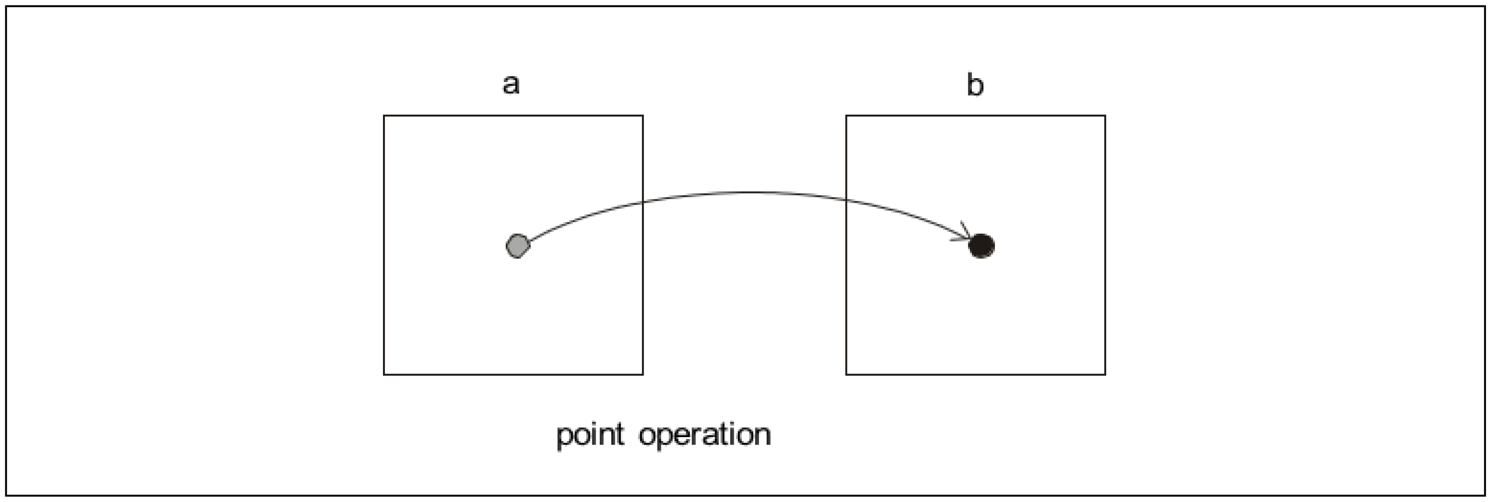
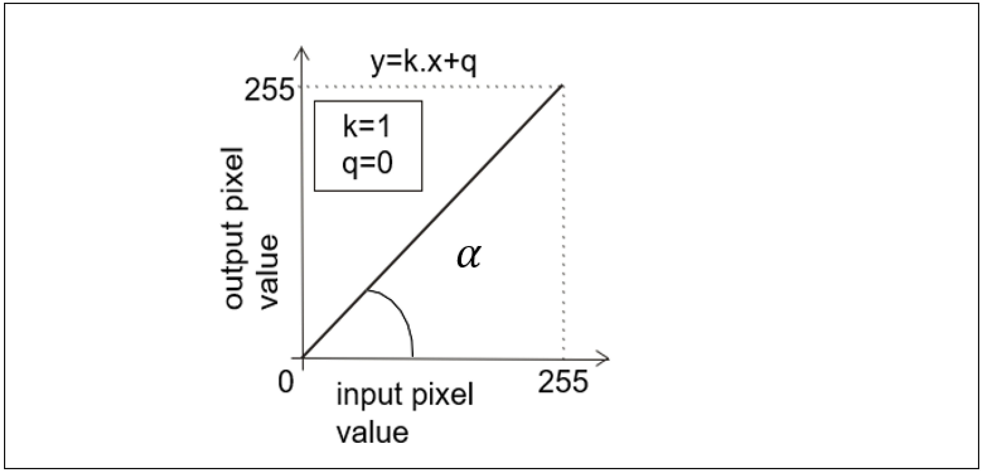
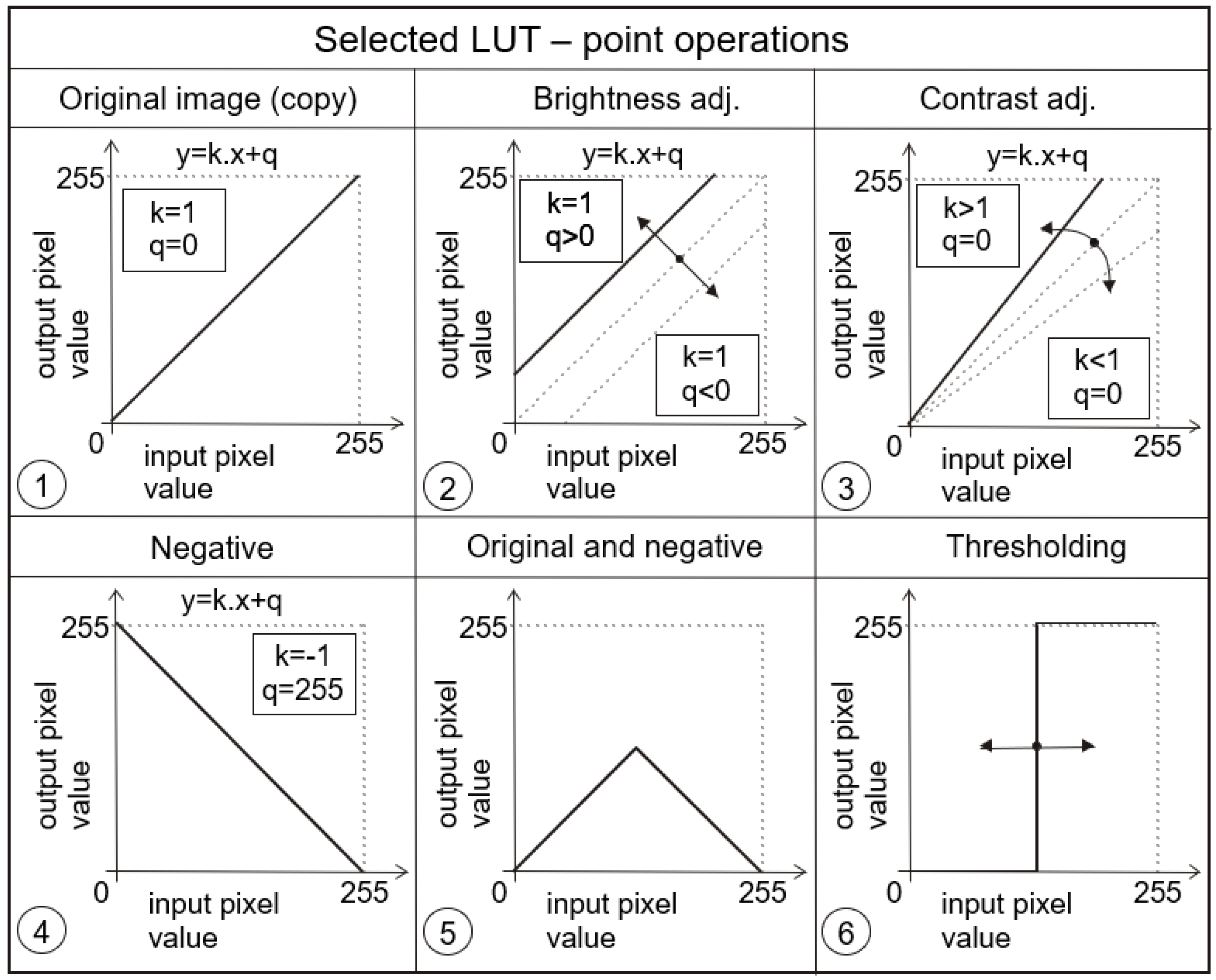
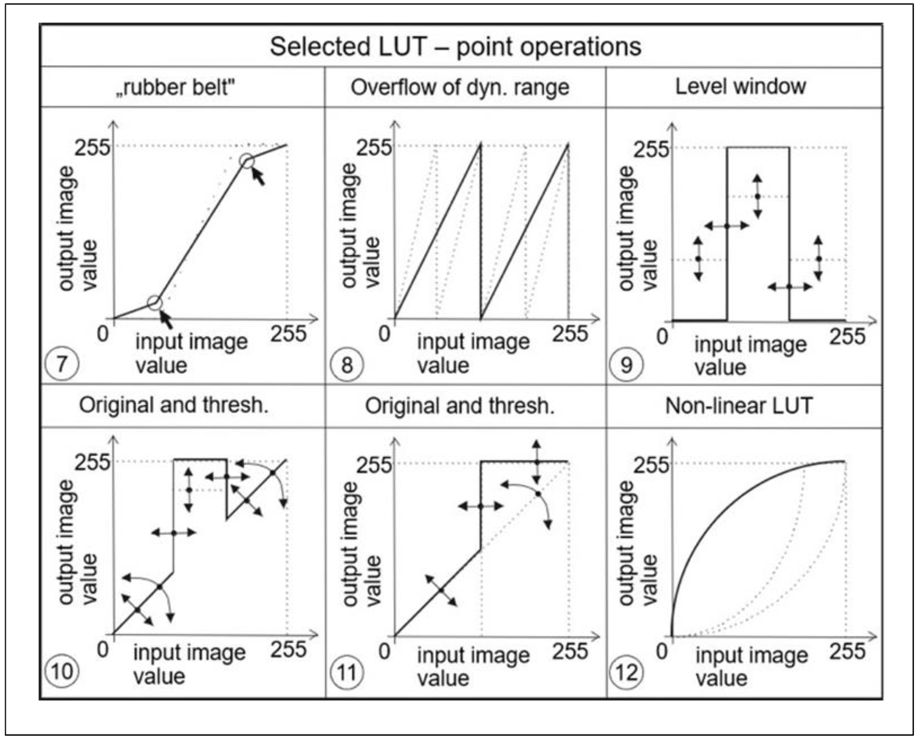
2.2.1. Transfer Functions, Resp. Look-up-Table Concept
Let us consider an experiment where we multiply the pixel values in the input image by 1. If we consider the usual input dynamic range of grayscale digital images (i.e., 0 to 255, where 0 represents the black level and 255 represents the white level), then the output image will produce a result that is identical to the values in the input image. For example, an input value of 10 would be multiplied by 1 and the result would also be 10 and this would continue for all pixel values in all positions. This then results in a simple linear function that can be represented as a straight line at a 45° angle and passing through the origin of the coordinates, or it is a simple copy of the input image. Such an example can also be expressed very simply in mathematical notation, namely the slope equation of the straight line as reported in Figure 3.
Figure 3.
Example of a point operator (function) that implements a copy of the input image on the output. In this case, the value of the slope (i.e., k = 1), and the value of the y-intercept of a straight line where a line crosses y-axis of a graph (i.e., q = 0).
With this defined operator, we can easily adjust various changes to image parameters such as brightness and contrast, both when we need to highlight selected gray levels or when we need to suppress them. Examples of different transfer functions are shown in Figure 4 and Figure 5.
Figure 4.
Examples of different point operators (functions) being very often used.
Figure 5.
Examples of other point operators (functions) that could also be utilized.
From the above examples, it is clear that these transfer functions or LUTs allow to significantly influence the visualization process of the given image data. Thus, for example, the transfer function in Figure 4 (panel 2) affects the brightness of the image, in Figure 4 (panel 3) it affects the contrast, in Figure 4 (panel 6) a transfer function for realizing a so-called binary image (i.e., an image that contains only two levels, most often black and white) is shown, and yet another suitable example can be seen in Figure 5 (panel 12), which is suitable for correcting an image that was taken under greatly reduced or increased lighting conditions. The latter two examples are further illustrated in the image data, respectively, in Figure 6 and Figure 7.
Figure 6.
Example of a point operator (function)—thresholding or binarization [16].
Figure 7.
Examples of point operator (function)—logarithmic function [16].
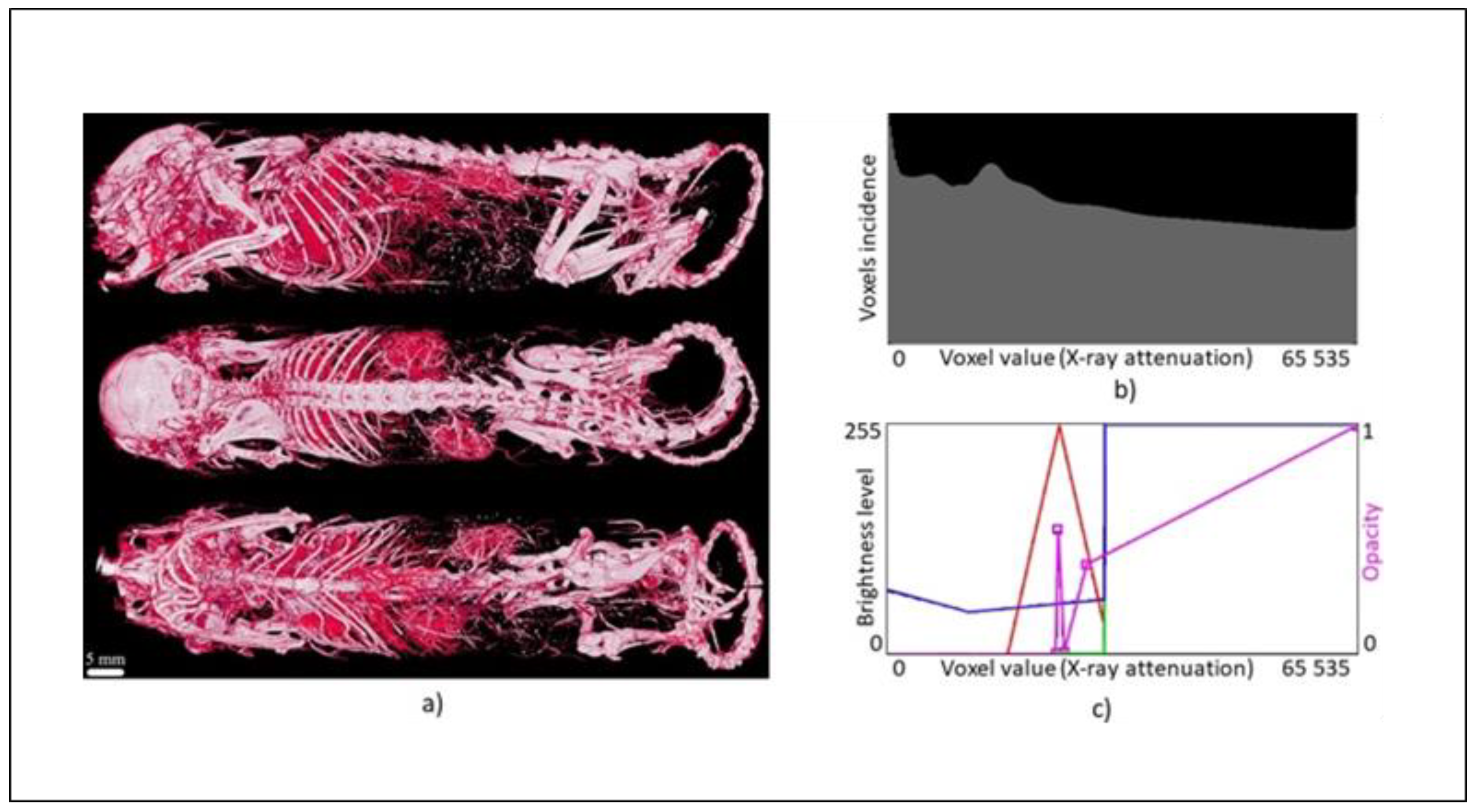
2.2.2. Transfer Functions Related to the Hounsfield Units (HU)
There is a very important process in CT and µCT imaging, that is the actual conversion of the attenuation of the passing X-rays to the grey level. Based on the physiological properties of human vision, 256 gray levels are very often used. The range of so-called Hounsfield units (HU) is typically in the range −1024 to +3071, which is 4096 values, and this is a much larger dynamic range than the 256 gray level values. For this reason, only the so-called windows on a given tissue (limited HU range), which has a width of 256 values or greater, need to be displayed. Thus, it is never possible to see all tissues at once, see soft tissue window, bone window, etc. Realistically, this situation is often implemented by a transfer function that has HU values on the x-axis and gray level values from 0 to 255 on the vertical axis. The situation is also depicted in Figure 8, which is an example of this situation in NRecon software [15].
Figure 8.
Nrecon SW MENU detail—reconstruction of outputs (parameter settings).
The practical impact of this situation is also the arrangement of the image data format in the form of so-called DICOM (Digital Imaging and Communications in Medicine) files. This file contains both image data and metadata [17] and each DICOM browser can display both. The structure of DICOM files consists of so-called tags and an example of these tags in relation to HU are the following items (i.e., the DICOM attribute number (0028,1053) whose name is “Rescale slope” and the DICOM attribute number (0028,1052) whose name is “Rescale intercept”). These parameters can then be substituted into the equation after the parameters k and q in Figure 3. These items can also be read.
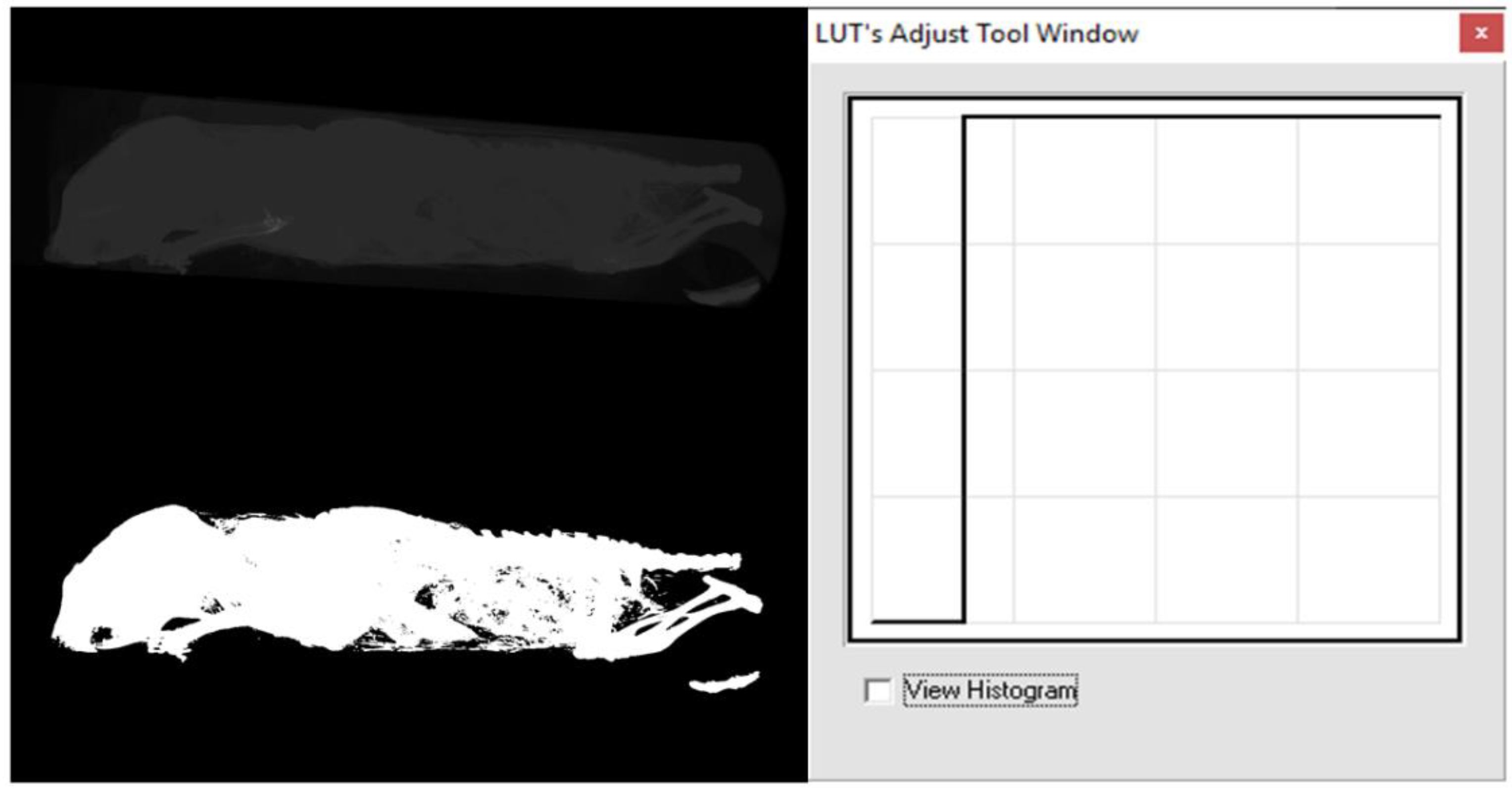
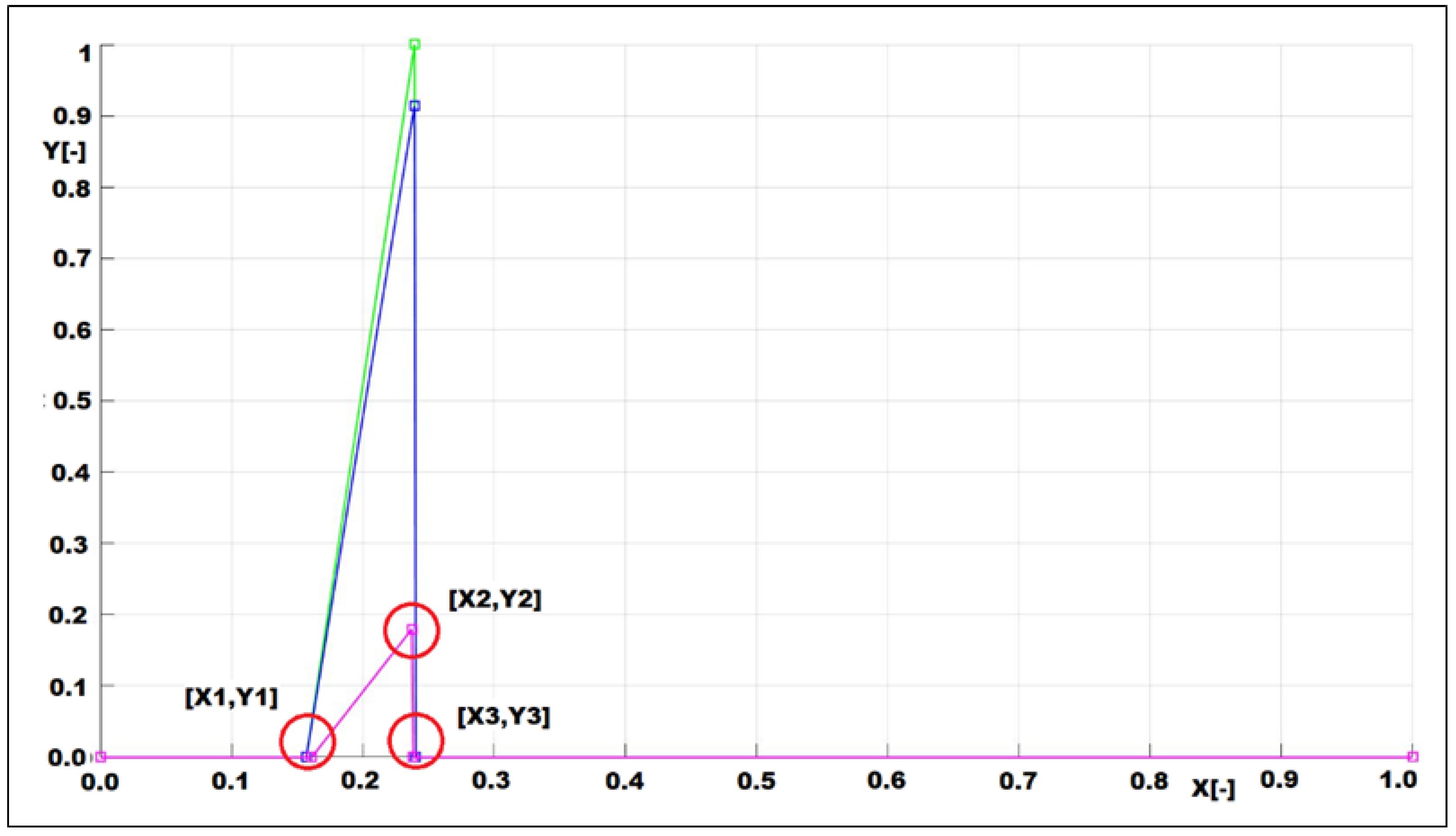
2.2.3. Transfer Functions Design Possibilities
Within the Ctvox software a histogram of the attenuation is available together with an editor that can be used to freely modify the transfer functions as LUTs, i.e., the program can either simply connect individual markers or use them as nodes to create a so-called spline curve. The program then assigns to each voxel the corresponding degree of the currently selected parameter (the so-called emission color [18]) depending on the attenuation of the voxel in the spline mode called volume rendering.
There are five parameters to choose from—opacity, red (R) channel, green (G) channel, blue (B) channel, and luminance (L), as reported in Figure 9c. If all three RGB channels are combined, only two parameters are available (i.e., opacity and luminance), and the voxels are assigned to their opacity and grayscale. In the other case, four parameters are available, namely, opacity together with all three RGB channels. In addition to assigning opacities, individual voxels can also be colored differently in this way, or segmented by color. In the case of opacity, there is available a purple opacity curve (initially a straight line, with just two markers) appears, in order to indicate that it is active. Opacity is the opposite of transparency. Hence, we will need to map low intensities to low opacities (i.e., high transparency), as shown in Figure 9c.
Figure 9.
Transfer functions design—(a) mouse (Aurovist, 42 kV), (b) histogram, and (c) transfer functions (opacity, RGB).
3. Results
A total of 53 transfer functions (LUTs) were designed, 42 of which were validated and optimized to emphasize the soft tissues of selected biological samples from µCT (mouse, rat, rabbit) using selected contrast agents (Aurovist, Omnipaque, KI in the ethanol solution, Mercox). The remaining 11 transfer functions could not be verified due to the absence of contrast in soft tissue samples from chickens. In total, 18 images and transfer functions are included within this text.
Out of the 53 transfer functions, one transfer function was able to be suggested that would likely highlight the tongue of a 19-day-old chick scanned with the Bruker SkyScan 1275 [19] at an anode voltage of 40 kV.
A total of 24 mice samples were statistically processed via correlation. Normality test was performed for all these samples in Matlab (Campus Wide Matlab, R2021a, The MathWorks, Inc., Natick, MA, USA) via Lilliefors test. These values were obtained for liver and kidneys of 24 mice in solutions of ethanol as a centroid value of the opacity LUT area under this graph (see example on Figure 10). Except for one dataset, all the others do not have a normal distribution according to this test. Results are available within Table 1, Table 2, Table 3 and Table 4 below. From this follows that there is required to use Spearman´s correlation coefficient.
Figure 10.
Example of the opacity (pink color) LUT with marked points that are used for computation of the centroid. Such figure exists for every included image (mouse_1_liver_ethanol_100_%_day_16).
Table 1.
p-values of the Lilliefors test of normality.
Table 2.
Ethanol liver raw data for centroid and Spearman´s correlation coefficient computation.
Table 3.
Ethanol kidney raw data for centroid and Spearman´s correlation coefficient computation.
Table 4.
Related parameters computed from raw data.
In Figure 10, we can see example of the opacity LUT with marked points, i.e., [X1,Y1], [X2,Y2], and [X3,Y3] whereby coordinate Y1 = 0 and Y3 = 0. These points form a homogenous triangle that enables simplified computation of the centroid.
The hypotheses mentioned within the Introduction were evaluated based on these data. This was a test of the alternative hypothesis that the Spearman correlation coefficient is not equal to 0. We used a relationship (see link within the [21]) where, given H0: r = 0, the t Student’s statistic has a distribution with d.f. (degree of freedom): N—2 (see also link within the [22]).
Ethanol liver: D.f.: 11, p-value: 0.3774 (for ethanol concentration) and D.f.: 11, p-value: 0.0001 (for days stored of the sample in ethanol solution).
Ethanol kidneys: D.f.: 9, p-value: 0.8504 (for ethanol concentration) and D.f.: 9, p-value: 0.00001 (for days stored of the sample in ethanol solution).
Overall, 18 LUTs from 53 LUTs were also validated on selected biological samples, selection of which is illustrated within this section and reported in Figure 9 and Figure 11, Figure 12, Figure 13.
Figure 11.
Transfer functions comparison—mouse (Aurovist, 42 kV).
Figure 12.
Contrast agents (left panels) and relevant transfer functions comparison (right panels): 1: Rat lungs and heart (Mercox, 34 kV); 2: Mouse hull (Aurovist, 42 kV); 3: Mouse liver (Omnipaque, 40 kV); and 4: Mouse brain (KI (potassium iodide) + Ethanol, 80 kV).
Figure 13.
Acquisition voltage comparison in 19 days old chicken. Ethanol, 100 kV (1–3) and 40 kV (4–6).
Due to the large number of results in the form of image data and transfer function, and due to the limited space for publication, only a few ones are presented below. Further significant visualizations, i.e., 18 examples, are available at higher resolution, i.e., with more details according to the contrast agent used, in Appendix A, specifically in Figure A1, Figure A2, Figure A3, Figure A4, Figure A5, Figure A6, Figure A7, Figure A8, Figure A9, Figure A10, Figure A11, Figure A12, Figure A13, Figure A14, Figure A15, Figure A16, Figure A17 and Figure A18. Part A1 (Figure A1 and Figure A2) is related to the ethanol contrast, part A2 (Figure A3, Figure A4, Figure A5, Figure A6 and Figure A7) to Aurovist, part A3 (Figure A8, Figure A9, Figure A10 and Figure A11) to Omnipaque, part A4 (Figure A12, Figure A13, Figure A14, Figure A15 and Figure A16) to potassium iodide (KI) in 20% ethanol solution and part A5 (Figure A17 and Figure A18) to Mercox resin. Captions of these figures content detailed descriptions of all possible findings due to the better contrast visualization. It is the reason why these figures are included with higher spatial resolution within the Appendix A.
4. Discussion
The main finding of this study is that there is a statistically significant monotonic relationship between the centroid of the area under the LUT curve and the number of days for which the animal sample was stored in the ethanol solution. H1 of the first hypothesis that the Spearman’s correlation coefficient does not equal zero (r1 ≠ 0) regarding this relationship was confirmed. On the other hand, there is no statistically significant monotonic relationship between the centroid of the area under the LUT curve and the concentration of the ethanol solution, see Table 1, Table 2, Table 3 and Table 4. In this case, H1 of the second hypothesis that the Spearman’s correlation coefficient does not equal zero (r2 ≠ 0) regarding this relationship was not confirmed. Within Table 4, we can see relevant average values for selected storage days of the specimen and related Hounsfield units, i.e., CT numbers as well. These values are very important and can be assigned to the centroid parameters of a LUT curve incorporating the relevant parameter of days for which the animal sample (mouse liver or kidney) was stored in ethanol solution.
Another finding of the study is that it is not possible to use one universal transfer function for proper soft tissue visualization of µCT images. The use of an appropriate contrast agent has a very significant effect on soft tissue visualization. It was possible to visualize the capillaries inside the chicken flesh in the phantom vasculature. In the case of the mouse heart, it was possible to segment and colorfully distinguish the tissue of the heart muscle from the rest of the blood vessels.
Due to the lack of one optimal and universal transfer function (LUT), a total of 53 transfer functions were designed using CTvox software [13] and optimized to highlight soft tissues in particular.
In the case of the mouse liver, mainly its external structures can be seen, while in the case of the kidney, brain, and heart, the internal structures are partially visible. In the mouse leg specimen, the transfer function emphasizes partly soft tissue and partly hard tissue (bone).
For the corrosive preparations, the soft tissue structures are shown by the contrast created between the Mercox resin and the air. Since the CT numbers of the synthetic resin are around 70 HU [2], it is possible to speak of a soft tissue equivalent in this case (range 40–80 HU).
Unfortunately, it was not possible to properly visualize soft tissues or organs from any of the chick scans. In fact, it is not certain that the scan of a stained chicken head of a 19-day-old chick at an anode voltage of 40 kV succeeded in highlighting just the tongue of this chick, or whether it is only the cartilaginous part of its beak.
In ex vivo samples of chickens prepared in ethanol and formaldehyde solutions, there was a presumption of contrast in the µCT images through protein coagulation. This assumption was probably only partially borne out and the result shows the interior of the chicken stained differently in blue and red, corresponding to a slight difference in CT numbers of otherwise further visualizable soft tissue. Furthermore, the ethanol solution in whole chickens did not have the opportunity to penetrate and subsequently evaporate from the animal cavities, which would have caused the solution to be replaced by air, which would have further caused better contrast in the µCT images (comparable to the evaporation of ethanol from the cavities of the animal organs evaporated therein).
It is also interesting to note that the plastic straw made of polyethylene has approximately the same CT number as the chicken meat and therefore cannot be distinguished from the meat as it passes through it. The glass capillary was the best of all materials to see, as the glass–air interface is a very high contrast object against soft tissue. This was followed by a larger diameter silicone capillary and the third was a smaller diameter capillary. Thus, in contrast to polyethylene, all other materials were clearly distinguishable from chicken meat (Figure 1).
In the majority of cases, the output of CTvox shows that using a lower anode voltage is the optimal choice for scanning soft tissue on µCT. In the case of bone segmentation, the choice of voltage did not play any significant role. For a more prominent presentation of the results, the processing of the oldest chicks prepared in ethanol was deliberately chosen, mainly because the chick is not sufficiently anatomically developed until around day 19 after egg fertilization, as this is the age at which chicks usually hatch. When younger chicks were examined, many structures were not yet sufficiently developed and, therefore, not visible.
Four chicken samples also contained the contrast agent Aurovist, consisting of 15 nm gold nanoparticles. Specifically, there were two scans at 10 days of age and another two at 12 days of age; unfortunately, no internal (soft) anatomical structures could be identified in this case either. This may have been due to the short age of the chicks, which may not have developed these structures properly yet. A second explanation could be that very low amount of Aurovist contrast agent was injected into the sample.
The limitation of this study is the relatively small number of included images and contrast agents. Another limitation is the use of the purely experimental-based level of visualization, i.e., there is subjective dependence of operator and possible variable deviation. In the case of statistical processing of the data with different KI concentrations, only two different concentrations were used—50% and 100%—this was a limitation, also.
5. Conclusions
In addition to the contrast agents used above, there is possible to use other more suitable contrast agents with very interesting properties. The idea is to perform next study based on the optimal contrast agent selection with relevant LUT. There are prepared comparative experiments with the set of such contrast agents as Sonovue, Iomeron, Optison, Omnipaque, Visipaque, Xenetix, Optiray, and Ultravist to be able to select appropriate one. However, there is assumed utilization of the semi-automatic/automatic LUT setup.
Author Contributions
Conceptualization and methodology, J.M. and J.H.; software, B.G.; validation, J.M. and P.Z.; formal analysis, J.R.; investigation, J.R.; resources, J.M.; data curation, J.M.; writing—original draft preparation, B.G. and J.H.; writing—review and editing, P.Z., G.G., A.L., A.M.; visualization, B.G.; supervision, P.Z.; project administration, J.M.; funding acquisition, J.M. All authors have read and agreed to the published version of the manuscript.
Funding
This research was funded by EU (European Regional Development Fund) and state budget of the Czech Republic, grant number CZ.02.1.01/0.0/0.0/16_019/0000766. The project was supported by Ministry of Education, Youth and Sports of the Czech Republic, Czech Technical University in Prague and Charles University.
Institutional Review Board Statement
The study was approved by the local Ethical Committees of the First and Third Faculty of Medicine, Charles University, Prague, Czech Republic (24185/2019). The animals were treated in accordance with the guidelines defined by the ethical committee, which follows the National Advisory Committee for Laboratory Animal Research (NAC LAR) guidelines. Handling of animals was performed in accordance with the Helsinki Declaration (seventh revision, 2013).
Informed Consent Statement
Not applicable.
Data Availability Statement
The complete original data are not publicly available due to large volume. However, there are available all LUTs as images and *.tf files and relevant images as well. Please, use the link within the [23].
Acknowledgments
There were used uncommercial licenses of software measure CT from Phywe [11,12], CTvox [13] and NRecon [15] from Bruker and Dragonfly [14] from ORS. We would like to thank Phywe, Bruker, and Object Research Systems for their kind support and feedback.
Conflicts of Interest
The authors declare no conflict of interest.
Appendix A
After reconstructing the data with NRecon, we designed several transfer functions in CTvox to emphasize the different structures of the selected samples, especially soft tissues. The CTvox outputs are divided into 5 subsections—according to the method of sample preparation or contrast used. This appendix is an additional section that contains details and data supplemental to the main text above (see the Results section). Figures of replicates for experiments of which representative data are shown in the main text above are added here with higher spatial resolution and detailed description.
Appendix A.1. Ethanol
For the preparations of chickens in ethanol solutions, we have designed transfer characteristics/functions highlighting their structures with different intensities of bone highlighting and then stained the samples with them.
Figure A1.
Dyed 19-day-old chicken (acquisition at anode voltage 100 kV, contrast agent ethanol). Ethanol fixed the surface structures of the soft tissues of the skin. The transition of the cartilaginous base of the skeleton (spine, skull, limbs) into bone forms is also shown.
Figure A2.
Dyed 19-day-old chicken (acquisition at anode voltage 40 kV, contrast agent ethanol). Imaging after 5 days of ethanol fixation with incipient soft tissue contrast of the trachea, diaphragm, and heart muscle. The contrast in this phase of fixation also corresponds to the density of the surface structures of skin derivatives (feathers).
Appendix A.2. Aurovist
In ex vivo mice with a gold nanoparticles contrast agent (Aurovist), we have designed transfer characteristics/functions that colorfully highlight soft tissue structures, particularly in blood vessels and airways.
Figure A3.
The Aurovist intravascular contrast displayed the entire vascular bed of the mouse. Here, is clearly visible the vasculature of the kidneys and their placement in the retroperitoneum on the sagittal section, the vessels of the thoracic organs, the hepatic vessels of all lobes, and the supply of the intestines in the abdominal cavity and pelvic plexus. In the section at the level of the thorax, there is a detail of the pulmonary system, where, according to the symmetry of the distribution and branching of the vessels, we can also describe their loss due to occlusion.
Figure A4.
Color resolution of mouse vessels on the body surface (red) and internal organs (green). This distinction also offers a comprehensive view important for the orientation and description of superficial and parietal vessels. In the head area is visible in the external carotid artery branching, then interscapular brown fat vessels, superficial thoracic branching of the thoracic artery and intercostal vessels, parietal lumbar and sacral vessels, as well as plexuses around the spinal canal and limb vessels. The blood vessels of the kidneys and liver here form a network corresponding to the location of the organs in the abdominal cavity, the blood vessels of the heart and lungs to the organs in the chest. This arrangement allows the vessels to be compared at different topographic sites in the body.
Figure A5.
Due to the intravascular contrast of Aurovist, a detailed section of the chest shows the vascular supply of the lungs and its perfusion. Simultaneous view of the bronchial tree allows comparison with respect to the ventilation of individual lung segments. Thus, it is possible to distinguish pathologies in the vascular system in terms of occlusion, embolism, or proliferation in tumor pathology and at the same time monitor the bronchial tree due to air contrast and pathology of reduced aeration in atelectasis and increased air space due to disruption of intrabronchial septum in emphysema.
Figure A6.
Detail view of the vascular system of the lungs in the chest of the mouse with Aurovist contrast in the sagittal and ventrodorsal scans and detail of the bronchial tree of the lung parenchyma in the same position. It is possible to compare pathologies in the vascular bed and bronchial branching separately.
Figure A7.
Transition of the thoracic and abdominal cavities and vascular supply of the lungs, heart, and the vessels of the liver and intestine. Simultaneous imaging of the bronchial ventilated tree helps to differentiate individual vascular systems. Detail of the hepatic vessels shows their segmentation into individual lobes. Another vascular system in the abdominal cavity corresponds to the largest perfusion in the bloodstream of the small and large intestine.
Appendix A.3. Omnipaque
In mouse organs prepared with Omnipaque contrast agent, transfer characteristics/functions highlighting the soft tissues of these organs were designed.
Figure A8.
Detailed view of the lobe of the liver and segmental vessels using Omnipaque contrast. Here, is a physiological finding. According to the drawing of the vasculature, we can also describe possible pathological conditions, reconstruction of the liver parenchyma, and its irregular vascular bed or proliferation of blood vessels in tumors.
Figure A9.
Ideal right lung position for imaging of bronchial branching down to alveolar levels using Omnipaque contrast. The right lung is rotated in a different position and it is possible that post-mortem it collapsed, mechanically vented, or was fixed in the fluid.
Figure A10.
Imaging of the capsule of the spleen and superficial vessels in fascial tissue in two positions using Omnipaque contrast.
Figure A11.
Imaging of superficial vessels of the epicardium and sub fascial layer of the heart.
Appendix A.4. Potassium iodide (KI) in 20% Ethanol Solution
To emphasize soft tissue organs loaded in a solution of dissolved potassium iodide in 20% ethanol solution, additional LUTs were designed and optimized.
Figure A12.
Imaging of the superficial capsule of the liver and division of the hepatic lobes.
Figure A13.
Iodine contrast and imaging of the kidney capsule, including the pathology of the cystic formation on the surface of the kidney.
Figure A14.
Imaging of the cerebral lobes and internal ventricular system with KI and 20% ethanol.
Figure A15.
Imaging of the epicardium and endocardium of the heart and its cavities with KI and 20% ethanol.
Figure A16.
Contrast of fascia muscle groups on the hind limb of mice with KI and 20% ethanol. The bones of the limb can be seen in detail, including the small tarsal bones of the foot.
Appendix A.5. Mercox (Resin)
For corrosive slides, transfer characteristics/functions emphasizing only the soft tissue structures (not the soft tissue itself) have been proposed using a contrast between resin and air. The images show the rabbit and rat airways, and in the case of the rat, the heart is visible along with the vasculature as well.
Figure A17.
Rabbit lung vessels visualized by Mercox contrast, a corrosive preparation. Here, the passage of blood vessels in post mortem is ensured by intravenous application of resin by continuous pressure. It is possible to modify vascular ligatures in experiments and, thus, display a failure that is similar to embolism. It is also possible to subsequently measure the angle of the segmental vessels distances and their diameters.
Figure A18.
The corrosive specimen of the heart and blood vessels shows both the coronary arteries for the heart, the basic platform for incipient myocardial infarction, and the branching of the pulmonary artery and pulmonary artery diameters and their angles of spacing and segmentation. Here, is a physiological finding. The arrangement of the pulmonary arteries and their branching is disturbed in pulmonary embolism, vascular wall pathology and also in lung tumors.
Appendix B
This appendix is an additional section that contains details and data supplemental to the main text from the point of view of the experimental setting of both setups, i.e., Phywe and Bruker systems.
Table A1.
Values of set parameters on the PHYWE XR 4.0 assembly.
Table A1.
Values of set parameters on the PHYWE XR 4.0 assembly.
| Parameter | Value | Physical Unit |
|---|---|---|
| object-source distance | 310 | mm |
| detector-source distance | 360 | mm |
| anode voltage | 35 | kV |
| emission current | 1 | mA |
| pixel projection dimension | 96 | μm |
| exposure time | 500 | ms |
| degree of rotation (increm.) | 1.8 | |
| binning 1 | 500 × 500 | pixels |
1 Explanation of binning is available within the [2,13].
The scan settings for scanning biological samples of chickens outside the shell with the SkyScan 1275 are shown in the following tables. The table header consists of a number followed by a capital letter D, this is the age of the chicken, which is given in days. This may be preceded either by another number followed by the capital letter E, in which case it is the concentration of the ethanol solution in which the chicken was prepared, or by the letter F, which indicates that the chicken was prepared in a formaldehyde solution. In four cases, the concentration of the Ethanol solution is preceded by the capital letter A, this is the contrast agent Aurovist.
Table A2.
Values of set parameters on SkyScan 1275.
Table A2.
Values of set parameters on SkyScan 1275.
| Parameter | Value 50E5D | Value 100E5D | Value F5D | Value 50E6D | Value 80E6D | Value 100E6D | Physical Unit |
|---|---|---|---|---|---|---|---|
| object-source distance | 40.97 | 40.97 | 40.97 | 40.97 | 40.97 | 40.97 | mm |
| detector-source distance | 286 | 286 | 286 | 286 | 286 | 286 | mm |
| anode voltage | 50 | 50 | 50 | 50 | 50 | 50 | kV |
| emission current | 200 | 200 | 200 | 200 | 200 | 200 | μA |
| pixel projection dimension | 11.6 | 11.6 | 11.6 | 11.6 | 11.6 | 11.6 | μm |
| exposure time | 50 | 50 | 50 | 50 | 50 | 50 | ms |
| degree of rotation (increm.) | 0.2 | 0.2 | 0.2 | 0.2 | 0.2 | 0.2 | |
| binning 1 | 1 × 1 | 1 × 1 | 1 × 1 | 1 × 1 | 1 × 1 | 1 × 1 | pixel |
1 Explanation of binning is available within the [2,13].
Table A3.
Values of set parameters on SkyScan 1275.
Table A3.
Values of set parameters on SkyScan 1275.
| Parameter | Value F6D | Value 80E7D | Value 100E7D | Value 80E8D | Value 80E9D | Value A80E10D | Physical Unit |
|---|---|---|---|---|---|---|---|
| object-source distance | 40.97 | 48.39 | 48.39 | 57.22 | 71.47 | 92.67 | mm |
| detector-source distance | 286 | 286 | 286 | 286 | 286 | 286 | mm |
| anode voltage | 50 | 50 | 50 | 65 | 70 | 100 | kV |
| emission current | 200 | 200 | 200 | 153 | 142 | 100 | μA |
| pixel projection dimension | 11.6 | 13.7 | 13.7 | 16.2 | 20.24 | 26.24 | μm |
| exposure time | 50 | 50 | 50 | 36 | 36 | 35 | ms |
| degree of rotation (increm.) | 0.2 | 0.2 | 0.2 | 0.2 | 0.2 | 0.2 | ° |
| binning 1 | 1 × 1 | 1 × 1 | 1 × 1 | 1 × 1 | 1 × 1 | 1 × 1 | pixel |
1 Explanation of binning is available within the [2,13].
Table A4.
Values of set parameters on SkyScan 1275.
Table A4.
Values of set parameters on SkyScan 1275.
| Parameter | Value A80E10D | Value 80E10-11D | Value 80E10-11D | Value 50E11D | Value 80E12D | Physical Unit |
|---|---|---|---|---|---|---|
| object-source distance | 71.47 | 60.75 | 67.9 | 92.67 | 80.4 | mm |
| detector-source distance | 286 | 286 | 286 | 286 | 286 | mm |
| anode voltage | 75 | 75 | 75 | 75 | 75 | kV |
| emission current | 133 | 133 | 133 | 133 | 133 | μA |
| pixel projection dimension | 20.24 | 17.2 | 19.23 | 26.24 | 22.77 | μm |
| exposure time | 36 | 36 | 36 | 36 | 500 | ms |
| degree of rotation (increm.) | 0.2 | 0.2 | 0.2 | 0.2 | 0.2 | ° |
| binning 1 | 1 × 1 | 1 × 1 | 1 × 1 | 1 × 1 | 1 × 1 | pixel |
1 Explanation of binning is available within the [2,13].
Table A5.
Values of set parameters on SkyScan 1275.
Table A5.
Values of set parameters on SkyScan 1275.
| Parameter | Value A80E12D | Value A80E12D | Value 50E13D | Value 50E14D | Value 100E14D | Physical Unit |
|---|---|---|---|---|---|---|
| object-source distance | 92.67 | 82.19 | 92.67 | 96.48 | 123.29 | mm |
| detector-source distance | 286 | 286 | 286 | 286 | 286 | mm |
| anode voltage | 75 | 75 | 75 | 75 | 80 | kV |
| emission current | 133 | 133 | 133 | 133 | 125 | μA |
| pixel projection dimension | 26.24 | 23.27 | 26.24 | 27.32 | 34.91 | μm |
| exposure time | 500 | 500 | 500 | 500 | 32 | ms |
| degree of rotation (increm.) | 0.2 | 0.2 | 0.2 | 0.2 | 0.2 | |
| binning 1 | 1 × 1 | 1 × 1 | 1 × 1 | 1 × 1 | 1 × 1 | pixel |
1 Explanation of binning is available within the [2,13].
Table A6.
Values of set parameters on SkyScan 1275.
Table A6.
Values of set parameters on SkyScan 1275.
| Parameter | Value 50E15D | Value 50E15D | Value 50E16D | Value 100E18D | Value 100E18D | Physical Unit |
|---|---|---|---|---|---|---|
| object-source distance | 146.51 | 142.94 | 178.67 | 169.74 | 176.89 | mm |
| detector-source distance | 286 | 286 | 286 | 286 | 286 | mm |
| anode voltage | 80 | 80 | 80 | 80 | 80 | kV |
| emission current | 125 | 125 | 125 | 125 | 125 | μA |
| pixel projection dimension | 41.48 | 40.47 | 50.59 | 48.06 | 50.08 | μm |
| exposure time | 32 | 32 | 32 | 33 | 33 | ms |
| degree of rotation (increm.) | 0.2 | 0.2 | 0.2 | 0.2 | 0.2 | ° |
| binning 1 | 1 × 1 | 1 × 1 | 1 × 1 | 1 × 1 | 1 × 1 | pixel |
1 Explanation of binning is available within the [2,13].
Table A7.
Values of set parameters on SkyScan 1275.
Table A7.
Values of set parameters on SkyScan 1275.
| Parameter | Value 100E19D | Value 100E19D | Value 100E19D | Value 100E19D | Physical Unit |
|---|---|---|---|---|---|
| object-source distance | 173.31 | 132.22 | 92.67 | 141.15 | mm |
| detector-source distance | 287 | 286 | 286 | 286 | mm |
| anode voltage | 40 | 80 | 100 | 100 | kV |
| emission current | 250 | 125 | 100 | 100 | μA |
| pixel projection dimension | 49.07 | 37.44 | 26.24 | 39.97 | μm |
| exposure time | 35 | 35 | 35 | 35 | ms |
| degree of rotation (increm.) | 0.2 | 0.2 | 0.2 | 0.2 | |
| binning 1 | 1 × 1 | 1 × 1 | 1 × 1 | 1 × 1 | pixel |
1 Explanation of binning is available within the [2,13].
The scanning parameters for scanning biological samples of chickens in the shell with the SkyScan 1275 are shown in the following tables. The table header consists of a number followed by a capital letter D, this is the age of the chicken, which is given in days.
Table A8.
Values of set parameters on SkyScan 1275.
Table A8.
Values of set parameters on SkyScan 1275.
| Parameter | Value 8D | Value 9D | Value 10D | Value 11D | Value 12D | Physical Unit |
|---|---|---|---|---|---|---|
| object-source distance | 155.45 | 146.51 | 151.87 | 137.58 | 153.66 | mm |
| detector-source distance | 286 | 286 | 286 | 286 | 286 | mm |
| anode voltage | 80 | 80 | 80 | 80 | 80 | kV |
| emission current | 125 | 125 | 125 | 125 | 125 | μA |
| pixel projection dimension | 44.01 | 41.48 | 43 | 38.95 | 43.51 | μm |
| exposure time | 36 | 36 | 36 | 36 | 36 | ms |
| degree of rotation (increm.) | 0.2 | 0.2 | 0.2 | 0.2 | 0.2 | |
| binning 1 | 1 × 1 | 1 × 1 | 1 × 1 | 1 × 1 | 1 × 1 | pixel |
1 Explanation of binning is available within the [2,13].
Table A9.
Values of set parameters on SkyScan 1275.
Table A9.
Values of set parameters on SkyScan 1275.
| Parameter | Value 13D | Value 14D | Value 15D | Value 15D | Value 16D | Physical Unit |
|---|---|---|---|---|---|---|
| object-source distance | 146.51 | 148.30 | 155.45 | 158.93 | 144.73 | mm |
| detector-source distance | 286 | 286 | 286 | 286 | 286 | mm |
| anode voltage | 80 | 80 | 80 | 80 | 80 | kV |
| emission current | 125 | 125 | 125 | 125 | 125 | μA |
| pixel projection dimension | 41.48 | 41.49 | 44.01 | 45 | 40.98 | μm |
| exposure time | 36 | 36 | 36 | 36 | 36 | ms |
| degree of rotation (increm.) | 0.2 | 0.2 | 0.2 | 0.2 | 0.2 | |
| binning 1 | 1 × 1 | 1 × 1 | 1 × 1 | 1 × 1 | 1 × 1 | pixel |
1 Explanation of binning is available within the [2,13].
Table A10.
Values of set parameters on SkyScan 1275.
Table A10.
Values of set parameters on SkyScan 1275.
| Parameter | Value 17D | Value 18D | Value 18D | Value 19D | Physical Unit |
|---|---|---|---|---|---|
| object-source distance | 159.02 | 157.23 | 167.95 | 150.09 | mm |
| detector-source distance | 286 | 286 | 286 | 286 | mm |
| anode voltage | 95 | 80 | 80 | 80 | kV |
| emission current | 105 | 125 | 125 | 125 | μA |
| pixel projection dimension | 45.03 | 44.52 | 47.55 | 42.50 | μm |
| exposure time | 36 | 36 | 36 | 36 | ms |
| degree of rotation (increm.) | 0.2 | 0.2 | 0.2 | 0.2 | |
| binning 1 | 1 × 1 | 1 × 1 | 1 × 1 | 1 × 1 | pixel |
1 Explanation of binning is available within the [2,13].
Table A11.
Values of set parameters on SkyScan 1275 for scanning of the 13 liver samples.
Table A11.
Values of set parameters on SkyScan 1275 for scanning of the 13 liver samples.
| Parameter | Value 50E8D | Value 50E17D | Value 100E8D | Value 100E16D | Value 100E37D | Physical Unit |
|---|---|---|---|---|---|---|
| object-source distance | 63.57 | 56.51 | 54.74 | 52.98 | 49.45 | mm |
| detector-source distance | 286 | 286 | 286 | 286 | 286 | mm |
| anode voltage | 30 | 40 | 30 | 35 | 40 | kV |
| emission current | 212 | 250 | 212 | 231 | 250 | μA |
| pixel projection dimension | 18.00 | 16.00 | 15.50 | 15.00 | 14.00 | μm |
| exposure time | 58 | 35 | 58 | 38 | 35 | ms |
| degree of rotation (increm.) | 0.2 | 0.2 | 0.2 | 0.2 | 0.2 | |
| binning 1 | 1 × 1 | 1 × 1 | 1 × 1 | 1 × 1 | 1 × 1 | pixel |
1 Explanation of binning is available within the [2,13].
Table A12.
Values of set parameters on SkyScan 1275 for scanning of the 11 kidneys samples.
Table A12.
Values of set parameters on SkyScan 1275 for scanning of the 11 kidneys samples.
| Parameter | Value 50E7D | Value 50E16D | Value 100E7D | Value 100E16D | Value 100E37D | Physical Unit |
|---|---|---|---|---|---|---|
| object-source distance | 28.26 | 28.26 | 30.02 | 28.26 | 28.26 | mm |
| detector-source distance | 286 | 286 | 286 | 286 | 286 | mm |
| anode voltage | 35 | 35 | 35 | 35 | 40 | kV |
| emission current | 231 | 231 | 231 | 231 | 250 | μA |
| pixel projection dimension | 8.00 | 8.00 | 8.50 | 8.00 | 8.00 | μm |
| exposure time | 35 | 38 | 35 | 38 | 35 | ms |
| degree of rotation (increm.) | 0.2 | 0.2 | 0.2 | 0.2 | 0.2 | |
| binning 1 | 1 × 1 | 1 × 1 | 1 × 1 | 1 × 1 | 1 × 1 | pixel |
1 Explanation of binning is available within the [2,13].
Table A13.
Values of set parameters on SkyScan 1275.
Table A13.
Values of set parameters on SkyScan 1275.
| Parameter | Value 17D | Value 18D | Value 18D | Value 19D | Physical Unit |
|---|---|---|---|---|---|
| object-source distance | 159.02 | 157.23 | 167.95 | 150.09 | mm |
| detector-source distance | 286 | 286 | 286 | 286 | mm |
| anode voltage | 95 | 80 | 80 | 80 | kV |
| emission current | 105 | 125 | 125 | 125 | μA |
| pixel projection dimension | 45.03 | 44.52 | 47.55 | 42.50 | μm |
| exposure time | 36 | 36 | 36 | 36 | ms |
| degree of rotation (increm.) | 0.2 | 0.2 | 0.2 | 0.2 | |
| binning 1 | 1 × 1 | 1 × 1 | 1 × 1 | 1 × 1 | pixel |
1 Explanation of binning is available within the [2,13].
Table A14.
Values of set parameters on SkyScan 1275.
Table A14.
Values of set parameters on SkyScan 1275.
| Parameter | Value 17D | Value 18D | Value 18D | Value 19D | Physical Unit |
|---|---|---|---|---|---|
| object-source distance | 159.02 | 157.23 | 167.95 | 150.09 | mm |
| detector-source distance | 286 | 286 | 286 | 286 | mm |
| anode voltage | 95 | 80 | 80 | 80 | kV |
| emission current | 105 | 125 | 125 | 125 | μA |
| pixel projection dimension | 45.03 | 44.52 | 47.55 | 42.50 | μm |
| exposure time | 36 | 36 | 36 | 36 | ms |
| degree of rotation (increm.) | 0.2 | 0.2 | 0.2 | 0.2 | ° |
| binning 1 | 1 × 1 | 1 × 1 | 1 × 1 | 1 × 1 | pixel |
1 Explanation of binning is available within the [2,13].
Table A15.
Values of set parameters on SkyScan 1275.
Table A15.
Values of set parameters on SkyScan 1275.
| Parameter | Value 17D | Value 18D | Value 18D | Value 19D | Physical Unit |
|---|---|---|---|---|---|
| object-source distance | 159.02 | 157.23 | 167.95 | 150.09 | mm |
| detector-source distance | 286 | 286 | 286 | 286 | mm |
| anode voltage | 95 | 80 | 80 | 80 | kV |
| emission current | 105 | 125 | 125 | 125 | μA |
| pixel projection dimension | 45.03 | 44.52 | 47.55 | 42.50 | μm |
| exposure time | 36 | 36 | 36 | 36 | ms |
| degree of rotation (increm.) | 0.2 | 0.2 | 0.2 | 0.2 | |
| binning 1 | 1 × 1 | 1 × 1 | 1 × 1 | 1 × 1 | pixel |
1 Explanation of binning is available within the [2,13].
Table A16.
Values of set parameters on SkyScan 1275.
Table A16.
Values of set parameters on SkyScan 1275.
| Parameter | Value 17D | Value 18D | Value 18D | Value 19D | Physical Unit |
|---|---|---|---|---|---|
| object-source distance | 159.02 | 157.23 | 167.95 | 150.09 | mm |
| detector-source distance | 286 | 286 | 286 | 286 | mm |
| anode voltage | 95 | 80 | 80 | 80 | kV |
| emission current | 105 | 125 | 125 | 125 | μA |
| pixel projection dimension | 45.03 | 44.52 | 47.55 | 42.50 | μm |
| exposure time | 36 | 36 | 36 | 36 | ms |
| degree of rotation (increm.) | 0.2 | 0.2 | 0.2 | 0.2 | ° |
| binning 1 | 1 × 1 | 1 × 1 | 1 × 1 | 1 × 1 | pixel |
1 Explanation of binning is available within the [2,13].
The scan settings for scanning mouse biological samples with Aurovist contrast agent (letter A), rabbit and rat biological samples with Mercox resin contrast agent (letter M), and mouse organ biological samples with Omnipaque contrast agent (letter O) and potassium iodide (KI) contrast agent dissolved in 20% ethanol solution (letters KI) with the SkyScan 1275 kit are shown in the following tables.
Table A17.
Values of set parameters on SkyScan 1275.
Table A17.
Values of set parameters on SkyScan 1275.
| Parameter | Value A-Mouse | Value M-Rabbit | Value M-Rat | Physical Unit |
|---|---|---|---|---|
| object-source distance | 92.67 | 148.30 | 62.54 | mm |
| detector-source distance | 286 | 286 | 286 | mm |
| anode voltage | 42 | 46 | 34 | kV |
| emission current | 238 | 217 | 227 | μA |
| pixel projection dimension | 26.24 | 41.99 | 17.71 | μm |
| exposure time | 99 | 35 | 41 | ms |
| degree of rotation (increm.) | 0.2 | 0.2 | 0.2 | ° |
| binning 1 | 1 × 1 | 1 × 1 | 1 × 1 | pixel |
1 Explanation of binning is available within the [2,13].
Table A18.
Values of set parameters on SkyScan 1275.
Table A18.
Values of set parameters on SkyScan 1275.
| Parameter | Value O-Liver | Value O-Lungs | Value O-Spleen | Value O-Heart | Physical Unit |
|---|---|---|---|---|---|
| object-source distance | 58.96 | 33.95 | 28.59 | 33.95 | mm |
| detector-source distance | 286 | 286 | 286 | 286 | mm |
| anode voltage | 40 | 54 | 54 | 40 | kV |
| emission current | 238 | 185 | 185 | 238 | μA |
| pixel projection dimension | 16.70 | 19.22 | 16.19 | 9.61 | μm |
| exposure time | 35 | 50 | 50 | 35 | ms |
| degree of rotation (increm.) | 0.2 | 0.4 | 0.4 | 0.2 | |
| binning 1 | 1 × 1 | 2 × 2 | 2 × 2 | 1 × 1 | pixels |
1 Explanation of binning is available within the [2,13].
Table A19.
Values of set parameters on SkyScan 1275.
Table A19.
Values of set parameters on SkyScan 1275.
| Parameter | Value KI-Liver | Value KI-Kidney | Value KI-Brain | Value KI-Heart | Value KI-Leg | Physical Unit |
|---|---|---|---|---|---|---|
| object-source distance | 107.21 | 32.16 | 117.93 | 39.31 | 178.67 | mm |
| detector-source distance | 286 | 286 | 286 | 286 | 286 | mm |
| anode voltage | 80 | 80 | 80 | 80 | 80 | kV |
| emission current | 125 | 125 | 125 | 125 | 125 | μA |
| pixel projection dimension | 30.36 | 9.11 | 33.39 | 11.13 | 50.59 | μm |
| exposure time | 35 | 35 | 35 | 35 | 35 | ms |
| degree of rotation (increm.) | 0.2 | 0.2 | 0.2 | 0.2 | 0.2 | |
| binning 1 | 1 × 1 | 1 × 1 | 1 × 1 | 1 × 1 | 1 × 1 | pixel |
1 Explanation of binning is available within the [2,13].
References
- Liguori, C.; Frauenfelder, G.; Massaroni, C.; Saccomandi, P.; Giurazza, F.; Pitocco, F.; Marano, R.; Schena, E. Emerging clinical applications of computed tomography. Med. Devices 2015, 8, 265–278. [Google Scholar] [CrossRef]
- Stock, S.R. Microcomputed Tomography: Methodology and Applications, 2nd ed.; CRC Press/Taylor and Francis: Boca Raton, FL, USA, 2020. [Google Scholar]
- Vickerton, P.; Jarvis, J.; Jeffery, N. Concentration-dependent specimen shrinkage in iodine-enhanced microCT. J. Anat. 2013, 223, 185–193. [Google Scholar] [CrossRef] [PubMed]
- Silva, J.M.D.E.; Zanette, I.; Noel, P.B.; Cardoso, M.B.; Kimm, M.A.; Pfeiffer, F. Three-dimensional non-destructive soft-tissue visualization with X-ray staining micro-tomography. Sci. Rep. 2015, 5, 14088. [Google Scholar] [CrossRef] [PubMed]
- Metscher, B.D. MicroCT for comparative morphology: Simple staining methods allow high-contrast 3D imaging of diverse non-mineralized animal tissues. BMC Physiol. 2009, 9, 11. [Google Scholar] [CrossRef] [PubMed]
- Patzelt, M.; Mrzilkova, J.; Dudak, J.; Krejci, F.; Zemlicka, J.; Karch, J.; Musil, V.; Rosina, J.; Sykora, V.; Horehledova, B.; et al. Ethanol fixation method for heart and lung imaging in micro-CT. Jpn. J. Radiol. 2019, 37, 500–510. [Google Scholar] [CrossRef] [PubMed]
- Dudak, J.; Zemlicka, J.; Karch, J.; Patzelt, M.; Mrzilkova, J.; Zach, P.; Hermanova, Z.; Kvacek, J.; Krejci, F. High-contrast X-ray micro-radiography and micro-CT of ex-vivo soft tissue murine organs utilizing ethanol fixation and large area photon-counting detector. Sci. Rep. 2016, 6, 30385. [Google Scholar] [CrossRef] [PubMed]
- McNitt-Gray, M.F.; Taira, R.K.; Johnson, S.L.; Razavi, M. An automatic method for enhancing the display of different tissue densities in digital chest radiographs. J. Digit. Imaging 1993, 6, 95–104. [Google Scholar] [CrossRef] [PubMed][Green Version]
- Seeram, E.; Seeram, D. Image Postprocessing in Digital Radiology—A Primer for Technologists. J. Med. Imaging Radiat. Sci. 2008, 39, 23–41. [Google Scholar] [CrossRef] [PubMed]
- Alshipli, M.; Kabir, N.A.; Hashim, R.; Marashdeh, M.W.; Tajuddin, A.A. Measurement of attenuation coefficients and CT numbers of epoxy resin and epoxy-based Rhizophora spp. particleboards in computed tomography energy range. Radiat. Phys. Chem. 2018, 149, 41–48. [Google Scholar] [CrossRef]
- Phywe XR 4.0 Expert Unit, X-ray Unit, 35 kV: Germany: PHYWE Systeme GmbH. Available online: https://repository.curriculab.net/files/bedanl.pdf/09057.99/0905799e.pdf (accessed on 18 July 2021).
- XR 4.0 Software Measure CT Manual. PHYWE. Available online: https://repository.curriculab.net/files/bedanl.pdf/14421.61/1442161e.pdf (accessed on 18 July 2021).
- CTvox Quick Start Guide. Bruker. Available online: https://www.bruker.com/fileadmin/user_upload/3-Service/Support/Preclinical_Imaging/X-Ray-uCT_Software/CTvox_QuickStartGuide.pdf (accessed on 18 July 2021).
- Key Features of Dragonfly. Available online: https://www.theobjects.com/dragonfly/features.html (accessed on 18 July 2021).
- NRecon User Manual. Available online: https://umanitoba.ca/faculties/health_sciences/medicine/units/cacs/sam/media/NReconUserManual.pdf (accessed on 18 July 2021).
- MIPS (Medical/Microscopy Image Processing Software). Available online: http://webzam.fbmi.cvut.cz/hozman/ (accessed on 20 February 2022).
- DICOM PS3.3 2021e—Information Object Definitions. C.11 LUT and Presentation States. Available online: https://dicom.nema.org/medical/dicom/current/output/chtml/part03/sect_C.11.2.htm (accessed on 28 November 2021).
- Weiss, S.; Westermann, R. Differentiable Direct Volume Rendering. IEEE Trans. Vis. Comput. Graph. 2022, 28, 562–572. [Google Scholar] [CrossRef] [PubMed]
- Skyscan CT-Volume Manual. Available online: https://umanitoba.ca/faculties/health_sciences/medicine/units/cacs/sam/media/CTVol_UserManual.pdf (accessed on 18 July 2021).
- Wolfram Research, Inc. Centroid of triangle–Wolfram Alpha. Wolfram Research, Inc., Champaign, IL. Available online: https://www.wolframalpha.com/input?i=centroid+of+triangle (accessed on 6 April 2022).
- Stakat. Let’s Master Statistics Together. Spearman’s Rho. Available online: https://statkat.com/stat-tests/spearmans-rho.php#5 (accessed on 25 April 2022).
- Real Statistics Using Excel. Spearman’s Rank Correlation Hypothesis Testing. Available online: https://www.real-statistics.com/correlation/spearmans-rank-correlation/spearmans-rank-correlation-detailed/ (accessed on 25 April 2022).
- Gaspar, B.; Mrzilkova, J.; Hozman, J.; Zach, P.; Lahutsina, A.; Morozova, A.; Guarnieri, G.; Riedlova, J. Data Availability Statement: There Are Available All LUTs as Images and *.tf Files and Relevant Images as Well. Available online: http://webzam.fbmi.cvut.cz/hozman/LUT.htm (accessed on 25 April 2022).
Publisher’s Note: MDPI stays neutral with regard to jurisdictional claims in published maps and institutional affiliations. |
© 2022 by the authors. Licensee MDPI, Basel, Switzerland. This article is an open access article distributed under the terms and conditions of the Creative Commons Attribution (CC BY) license (https://creativecommons.org/licenses/by/4.0/).