Article

Identification of Wiener Box-Jenkins Model for Anesthesia Using Particle Swarm Optimization

1
Biomedical Engineering Department, Imam Abdulrahman Bin Faisal University, Dammam 31441, Saudi Arabia
2
Department of Computer and Systems Engineering, Zagazig University, Zagazig 44519, Egypt
*
Author to whom correspondence should be addressed.
Appl. Sci. 2022, 12(10), 4817; https://doi.org/10.3390/app12104817
Submission received: 15 April 2022 / Revised: 29 April 2022 / Accepted: 4 May 2022 / Published: 10 May 2022
(This article belongs to the Special Issue Distributed Control for Robotics)

Abstract

:
Anesthesia refers to the process of preventing pain and relieving stress on the patient’s body during medical operations. Due to its vital importance in health care systems, the automation of anesthesia has gained a lot of interest in the past two decades and, for this purpose, several models of anesthesia are proposed in the literature. In this paper, a Wiener Box-Jenkins model, consisting of linear dynamics followed by a static polynomial nonlinearity and additive colored noise, is used to model anesthesia. A set of input–output data is generated using closed-loop simulations of the Pharmacokinetic–Pharmacodynamic nonlinear (PK/PD) model relating the drug infusion rates, in [μgkg−1min−1], to the Depth of Anesthesia (DoA), in [%]. The model parameters are then estimated offline using particle swarm optimization (PSO) technique. Several Monte Carlo simulations and validation tests are conducted to evaluate the performance of the identified model. The simulation showed very promising results with a quick convergence in less than 10 iterations, with a percentage error less than 1.5%.

1. Introduction

Anesthesia is the process of preventing the pain and mitigating the stress of the patient’s body to injury during medical operations [1]. The process is conducted by injecting gases and/or drugs by a specialist before and during surgical operations. Anesthesia can be performed by inhalationof smelled gases or intravenous injections using needles [2]. As a result of the advanced devices available in the market for inhalation, the current study is focused on intravenous anesthesia. In both cases, the process can be divided into three stages: (1) induction, which starts from administration of drug to the patient until he/she reaches unconsciousness, (2) maintenance during which the surgery is performed, and (3) recovery, in which the patient regains consciousness [3].
The use of advanced control and automation in anesthesia focuses on the maintenance stage in order to inject the correct dosage, which keeps the level of patient’s unconsciousness within safe limits during operations. This is of vital importance, especially if there is a shortage of anesthesiologists in, e.g., war times, natural disasters, or remote areas [4]. The level of Anesthesia is usually expressed in terms of the so-called Depth of Anesthesia (DoA), which measures the degree of suppression of the central nervous system [1]. Various techniques have been used for the control of the DoA including Proportional Integral Derivative (PID) [5,6,7], fractional PI [8], model predictive controller (MPC) [9], and neuro-fuzzy control [10].
Attempts to model DoA began around the middle of the twentieth century through monitoring brain activity using Electroencephalogram (EEG) signal. Later, in the eighties, other attempts are made predominantly on inhaled anesthesia [11]. In the past two decades, modeling of intravenous anesthesia received more attention from researchers [3,5,9,12,13,14,15,16,17,18,19,20,21,22,23]. Although there are attempts to use linear models such as [24], most of the proposed models are nonlinear, employing a linear transfer function subsystem followed by the so-called hill static nonlinearity function. This model structure is termed Wiener model in the system identification literature and is widely used in the modeling of anesthesia [2,3,14,16,23,25].
One common model approximating the DoA process and giving deep insight is the so-called Pharmacokinetic-Pharmacodynamic nonlinear model (PK/PD), where the infusion rates of the propofol and remifentanil are the input signals and the DoA obtained by the spectral Bispectral index (BIS), which monitors the depth of anesthesia, is the output. The approximated model is represented by Wiener model, where the PK part comprises the linear dynamic subsystem in cascade with PD static nonlinearity [21,22]. There are few iterative approaches to model drug dynamics during anesthesia such as artificial neural network [13] where the prediction results are very promising, however, the method did not perform well due to the presence of delays in this application. Additionally, the multi-input multi-output (MISO) output error model using closed loop instrumental variables (IV) method is employed [18]. Although this approach is favorable to the black-box neural network model, it is not very accurate either.
As the PK/PD model of drug dynamics during anesthesia consists of linear block followed by nonlinearity, it is proposed, in this paper, to use the Wiener Box-Jenkins model to the relationship between the infusion rate of muscle relaxant, e.g., atracurium, u ( t ) in [μgkg−1min−1] and the level of neuromuscular blockader NMB or DoA in [%]. By simulating the process in closed-loop configuration, a set of input–output data, sampled every 0.1 min, is generated to be used in offline identification of model parameters. The model parameters are estimated by minimizing the mean square one-step ahead prediction error (MSE) using Particle Swarm Method (PSO), a very successful meta-heuristic optimization technique [26,27,28]. The main contribution of this paper is to use the Wiener Box-Jenkins model to approximate the mathematical model of anesthesia using simulated model data and employing the PSO-based optimization technique to estimate the parameters of the empirical model.
This paper is organized as follows. First, the minimally parameterized parsimonious (MPP) model for drug dynamics during anesthesia is reviewed in Section 2. In Section 3, the Wiener Box-Jenkins model is presented and its one-step ahead prediction error is formulated. The section concludes with a review of the PSO algorithm to be used for estimating model parameters. The simulation setup and results are elaborated in Section 4. Finally, a summary and suggested future research are provided in Section 5.

2. MPP Anesthesia Model Description

The modeling of drug dynamics during anesthesia concentrates on describing the gap between the plasma concentration and consequence of the drug delivery. One common model for this purpose is the PK/PD model which can be simplified to the minimally parametrized parsimonious (MPP) model presented in da Silva [4]. The model describes the relationship between the infusion rate of muscle relaxant, e.g., atracurium, u ( t ) in [μgkg−1min−1] and the resulting level of neuromuscular blockade r ( t ) in [%].
The MPP model consists of a linear subsystem cascaded by a nonlinear function. The linear subsystem is approximated by the following third-order state space model:
d x 1 ( t ) d t = k 3 α x 1 ( t ) + k 3 α u ( t ) d x 2 ( t ) d t = k 2 α x 1 ( t ) k 2 α x 2 ( t ) d x 3 ( t ) d t = k 1 α x 2 ( t ) k 1 α x 3 ( t )
where x 1 , x 2 and x 3 denote system states in [μgmL−1], k 1 , k 2 and k 3 are parameters that have been suitably determined by Silva [4] for atracurium, and α > 0 is a patient-dependent parameter.
The nonlinear subsystem can be described using the following so-called hill function:
r ( t ) = 100 · C ¯ 50 γ C ¯ 50 γ + x 3 γ ( t )
where the parameter C ¯ 50 , in [μgmL−1] denotes the half of maximum effect concentration and has a fixed value of 3.2425 [29], and γ is another patient-dependent parameter.
Although, the MPP model given by Equations (1) and (2) has a clear interpretation, the estimation of its parameters is not straightforward. This was the motivation of the current paper to employ system identification techniques which, although being black box, can be applied directly to measured input–output data and provide quick and accurate description of the dynamics of the anesthesia process.

3. System Identification

In this section, the Wiener Box-Jenkins model structure is presented. The prediction error cost function of the model is then formulated. Finally, the PSO iterative optimization technique, which is used for estimating model parameters, is reviewed.

3.1. Wiener Box-Jenkins Model Structure

The Wiener Box-Jenkins model is shown in Figure 1, where it consists of a linear dynamic subsystem, G ( z 1 ) , in cascade with a static non-linearity, m ( · ) . The noise model H ( z 1 ) is fed by a white noise sequence e ( t ) to yield a colored noise v ( t ) [30,31].
The output of the linear process part is given by
x ( t ) = G ( z 1 ) u ( t )
where u ( t ) is the model input. The model output y ( t ) is expressed as
y ( t ) = y d ( t ) + v ( t )
where the colored noise v ( t ) is given as
v ( t ) = H ( z 1 ) e ( t )
and y d ( t ) is the undisturbed process output calculated as
y d ( t ) = m ( x ( t ) ) = i = 0 M β i x i ( t ) .
where the coefficients, β i , i = 0 M , are the parameters of the polynomial nonlinearity m ( · ) of order M. Other types of basis expansions, such as orthogonal polynomials [32] or splines [33], could also be used.
The linear filters G ( z 1 ) and H ( z 1 ) are defined as:
G ( z 1 ) = B ( z 1 ) F ( z 1 ) ,
H ( z 1 ) = C ( z 1 ) D ( z 1 ) ,
where the numerators and denominators, B ( z 1 ) , F ( z 1 ) , C ( z 1 ) , and D ( z 1 ) , are polynomials in the discrete shift operator z 1 as follows:
B ( z 1 ) = b 0 + b 1 z 1 + + b n b z n b F ( z 1 ) = 1 + f 1 z 1 + + f n f z n f C ( z 1 ) = 1 + c 1 z 1 + + c n c z n c D ( z 1 ) = 1 + d 1 z 1 + + d n d z n d
It is assumed that the maximum degree of the elements n b , n a , n c , and n d , and M are selected a priori and the noise filter H ( z 1 ) is stable and inversely stable. For systems with time delay of l samples, the leading numerator parameters, b 0 , b 1 , , b l 1 , would be zero. Detailed formulations of the Wiener Box-Jenkins model are available in [34].

3.2. Prediction Error Method (PEM)

The parameters for the Wiener Box-Jenkins model can be collected in the following vector
θ = [ b 0   b 1 b n b   f 1 f n f   c 1 c n c   d 1 d n d β 0     β M ]
In PEM setting, the parameter vector θ is optimized in such a way to minimize the error, i.e., the difference between the measured and predicted output. The one step ahead predictor (OSAP) is commonly used, where the current output at time instant t is predicted given input and output values up to time instant t 1 . The OSAP of the proposed Wiener Box-Jenkins model can be expressed as follows:
y ^ ( t | t 1 , θ ) = y d ( t , θ ) + v ^ ( t | t 1 , θ )
where the OSAP for the noise part is found from
v ^ ( t | t 1 , θ ) = H ( z 1 ) 1 H ( z 1 ) v ( t , θ ) = 1 H 1 ( z 1 ) v ( t , θ )
and the deterministic part is computed using Equation (5).
By substituting the formulas of v ^ ( t | t 1 , θ ) and y d ( t , θ ) , the one-step ahead predicted output is given by [30]:
y ^ ( t | t 1 , θ ) = 1 H 1 ( z 1 ) y ( t ) + H 1 ( z 1 ) i = 0 M β ( i ) G ( z 1 ) u ( t ) i = C ( z 1 ) D ( z 1 ) C ( z 1 ) y ( t ) + D ( z 1 ) C ( z 1 ) i = 0 M β ( i ) B ( z 1 ) A ( z 1 ) u ( t ) i
The prediction error of the model ϵ ( t ) is, therefore, given by
ϵ ( t ) = y ( t ) y ^ ( t | t 1 , θ ) = H 1 ( z 1 ) y ( t ) y d ( t , θ ) .
Usually, the mean square error (MSE) cost function, defined as
V N ( θ ) = 1 2 N t = 1 N ϵ 2 ( t , θ ) ,
is used to assess the performance of the model. The objective of PEM method is to search for the parameter vector θ that minimizes V N ( θ ) , that is
θ ^ = arg   min θ   V N ( θ )
The challenge is that some parameters such as the elements of C ( z 1 ) and A ( z 1 ) appears nonlinearly in the the predictor y ^ ( t | t 1 , θ ) defined by Equation (12). Therefore, an iterative optimization technique is needed. In this paper, PSO meta-heuristic optimization technique is employed for the estimation of the parameter vector (9) such it minimizes the cost function (14). The details of the PSO algorithm are elaborated next.

3.3. Iterative Optimization Using PSO

PSO optimization algorithm (PSO), proposed by Kennedy and Eberhart [26], is one of the meta-heuristic based optimization approaches that gained a lot of interest in the literature with many successful applications [26,27,28]. One major advantage of meta-heuristic algorithms is that they are derivative-free. This is in contrast to classical optimization techniques such as gradient descent or Newton methods, which require first and sometimes second derivatives of the predictor with respect to the parameter vector.
In PSO algorithm, a set or population of candidate solutions, called particles, are considered in at each iteration in an attempt to explore the search space. Based on the information gathered in each iteration, the current solutions are updated, and a new population is created. The best global solution at each iteration is recorded. The algorithm terminates when the improvement in the best solution is below some specified tolerance, or if the maximum number of iterations is reached.
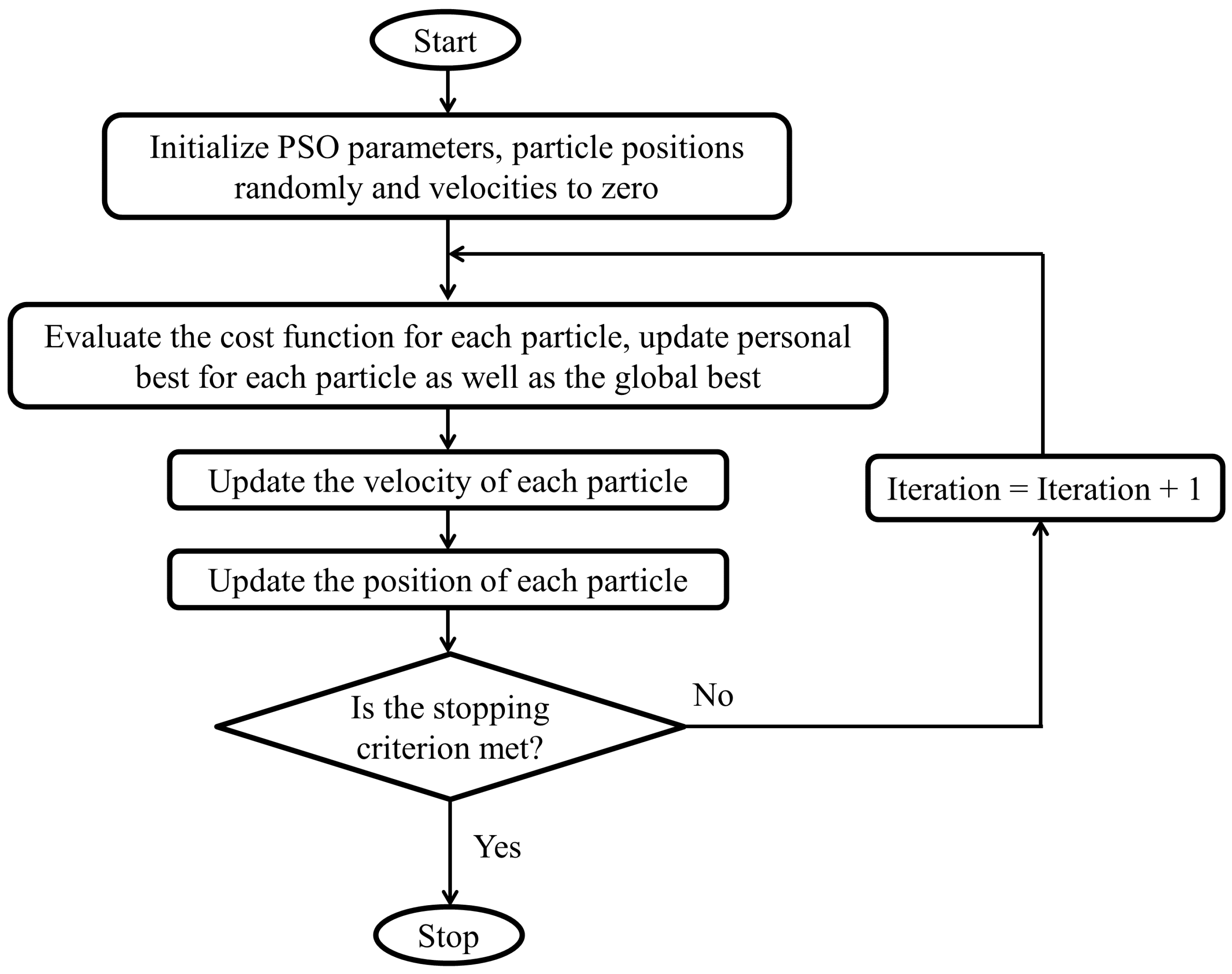
The PSO algorithm, illustrated in Figure 2, can be summarized as follows [35]:
  • Generate, randomly, a population of initial parameter vectors, solutions, or particles, θ i ( 0 ) , for i = 1 , 2 , , N p , where N p is the population size. Each entry in the vector θ i ( 0 ) is initialized to a random number generated from a uniform distribution in the interval [ θ M i n , θ M a x ] where θ M i n and θ M a x denote the lower and upper bounds, respectively, of the parameters. Additionally, initialize the velocity, V i ( 0 ) , for each particle in the population, to zero.
  • Evaluate the cost function given by (14) for each particle θ .
  • Update the best value p b e s t i for each particle i by comparing the current cost of each particle with its previous best value.
  • Update the population’s best value g b e s t .
  • Update the velocity of each particle using the following formula:
    V i ( t + 1 ) = w V i ( t ) + c 1 r 1 ( t ) ( p b e s t i θ i ( t ) ) + c 2 r 2 ( t ) ( g b e s t θ i ( t ) ) ,
    where V i ( t + 1 ) and V i ( t + 1 ) denotes the velocity of particle i at iterations t + 1 and t, respectively. The parameters r 1 , and r 2 are two random numbers, and c 1 and c 2 are two positive constants called the personal and global acceleration coefficients. The parameter w, called the inertia weight, controls the effect of the current particle solution on its next solution. The inertia weight is damped in each iteration using the following formula:
    w = w ζ d a m p ,
    where ζ d a m p denotes the damping ratio of the inertia coefficient.
  • Update each particle position using the following formula:
    θ i ( t + 1 ) = θ i ( t ) + V i ( t + 1 )
  • If the change in g b e s t is less than some given small tolerance or the maximum number of iterations is reached, the algorithm terminates; otherwise, go to step 2).
    The settings for the parameters of the PSO algorithm to be used in this paper are listed in Table 1. More information about the selection the PSO parameters were explained in [36].

4. Simulation Results

In order to identify the Wiener Box-Jenkins model, Figure 1, a set of input–output data is collected for the MPP anesthesia model under closed loop PID control. In this section, the simulation setup for data collection is first described and, then, the identification results of the Wiener Box-Jenkins model are presented.

4.1. Data Collection

To generate the required input-output data, the patient model (1) and (2) is simulated under closed-loop PID control as shown in the block diagram of Figure 3. In the figure, the set point is the desired level of neuromuscular blockade (NMB), r ( t ) is the actual level of NMB measured by the supra-maximal train-of-four (TOF) stimulation of the ulnar nerve, e ( t ) is the error or difference between the desired and actual NMB, and the atracurium infusion rate is denoted by u ( t ) [2].
The transfer function of the PID controller used is expressed as
u ( t ) = K e ( t ) + 1 T i 0 t e ( τ ) d τ + T d d e ( t ) d t ,
where the parameters K, T i , and T d are the controller gain, integral time, and derivative time, respectively. In practice, the derivative term is filtered using a first-order filter
G f ( s ) = T d s T d N s + 1 ,
where the derivative gain N is usually set to 10. The settings for both the PID controller gains and the parameters for patient number 17 in the MPP dataset [37] are listed in Table 2.
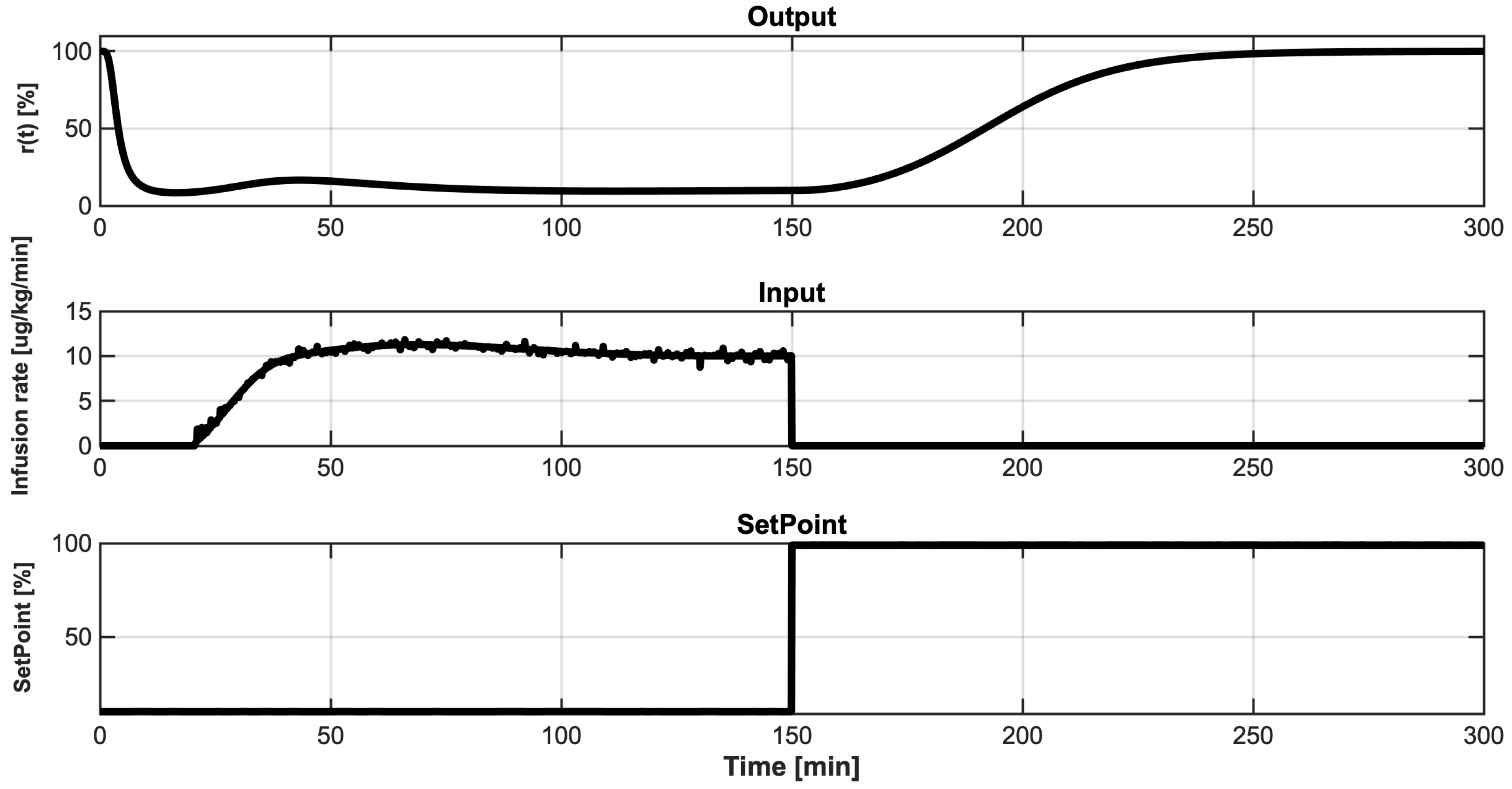
One hundred Monte Carlo simulation runs of the MPP body model response to muscle relaxants are conducted using a sample period of 0.1 min. The length of each run is 300 min, in which in the first 150 min, the set-point is 10% corresponding to the maintenance phase. It should be noted that before the start of the maintenance phase, an initial induction of a standard 500 [μg/kg] drug bolus is used. After the injection of the initial bolus, the PID controller starts to operate after 20 min. The output of the PID controller is normalized with respect to the patient weight (70 kg) and bounded by a saturation block representing infusion limits [37]. The remaining 150 min of each run represent the recovery phase where the set-point is set to 99%.
An independent sequence of binary random numbers (value ± 1) are filtered using the following first-order filter:
G ( z ) = 0.05 1 0.5 z 1 ,
and added to the set-point in the whole 300 min period. The reason for using the filter is to avoid large control signals due to the derivative action. The atracurium infusion rate, u ( t ) , in [μg/kg], and the level of neuromuscular blockade (NMB), and the reference signal are shown in Figure 4, in one sample run.

4.2. Identification Results

In this section, the results of the offline identification of Wiener Box-Jenkins structure for MPP anesthesia model are presented, analyzed, and validated.
The model is used to fit the input–output data collected in Section 4.1. The linear parts of the model were approximated by two transfer functions: a second-order process transfer function G ( z 1 ) and a first-order noise model H ( z 1 ) . In addition, the Hill nonlinearity is captured using a third-order polynomial nonlinearity, where the order is selected manually.
The estimates of Wiener Box-Jenkins model parameters averaged over one hundred runs are listed in Table 3.
There are several indices used to evaluate model prediction. One example is the percentage variance accounted for (% V A F ), calculated as
% V A F = 1 E [ ( y ( t ) y ^ ( t ) ) 2 ] E [ ( y ( t ) y ¯ ( t ) ) 2 ] × 100 %
where y ( t ) is the measured output and y ^ ( t ) is the model output. Another index is the mean absolute error ( M A E ) given by
M A E = 1 N t = 1 N | y ( t ) y ^ ( t ) |
where N is the total number of data samples. Closely related to MAE is the mean absolute percentage error ( M A P E ) computed by the following formula:
M A P E = 1 N t = 1 N | y ( t ) y ^ ( t ) | y ^ ( t )
Lastly, the coefficient of determination ( R 2 ) is defined as:
R 2 = 1 1 N t = 1 N | y ( t ) y ^ ( t ) | 2 1 N t = 1 N | y ( t ) y ¯ ( t ) | 2
where
y ¯ ( t ) = 1 N t = 1 N y ( t )
The mean square error, (%VAF), mean absolute error (MAE), mean absolute percentage error (MAPE), and the coefficient of determination ( R 2 ) are given in Table 4. Again, it can be realized that the %VAF is close to 100% and R 2 to unity. Additionally, the MAPE error is very small. These all confirm the precision of the Wiener Box-Jenkins model in modeling drug delivery.
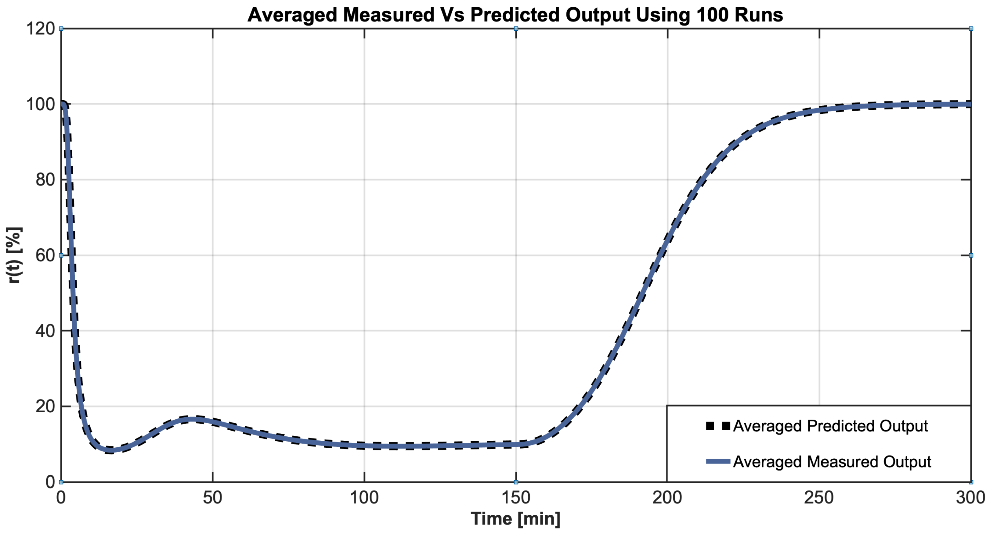
Furthermore, the average measured and predicted output of NMB outputs are shown in Figure 5. It is clear that the PSO optimization-based prediction is close to measured output with MSE average cost function using 100 run is 0.0127 .
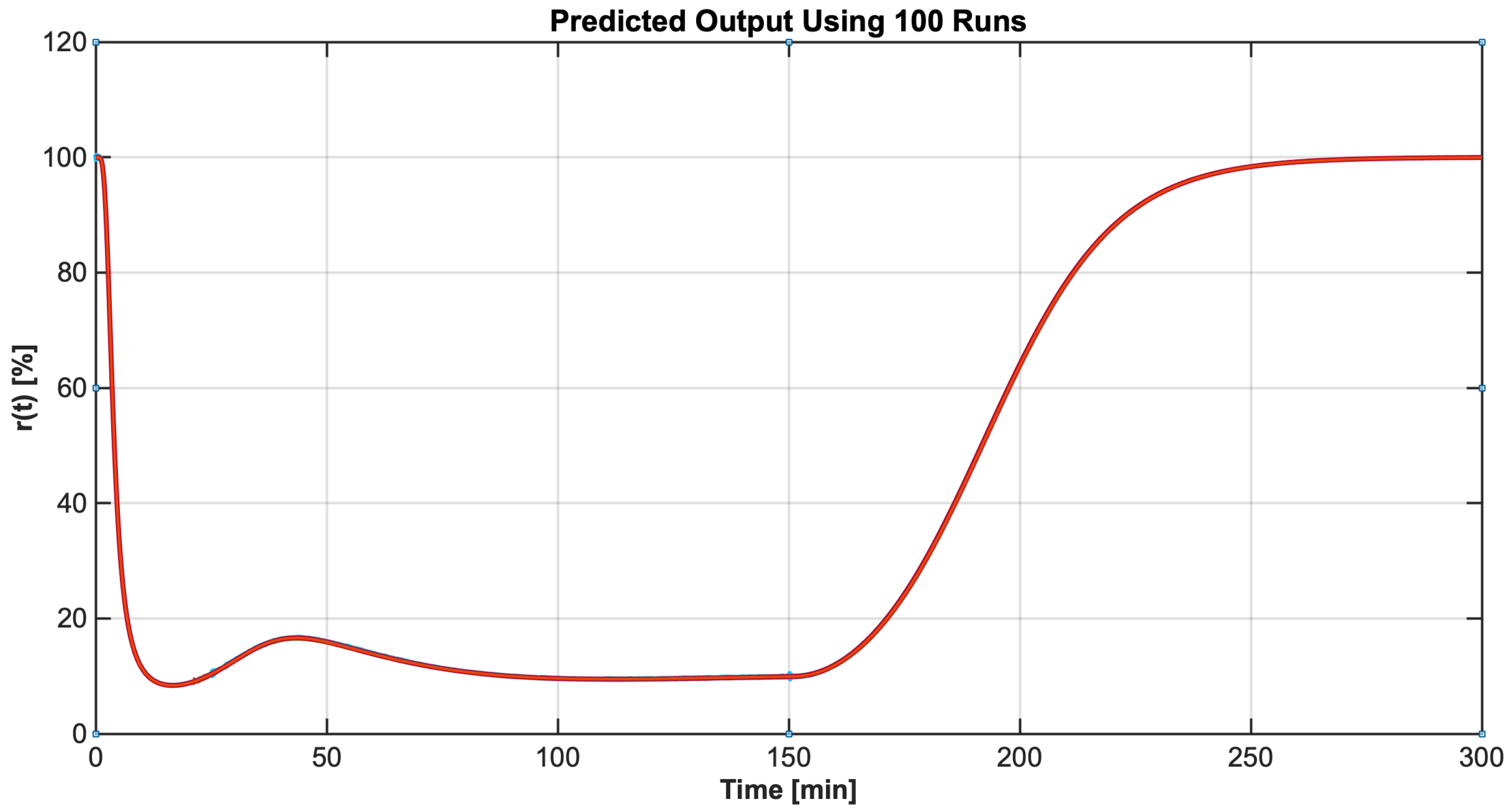
Additionally, the predicted output in 100 Monte Carlo runs are shown in Figure 6. The output in all runs fits well together, showing the consistency of the model.
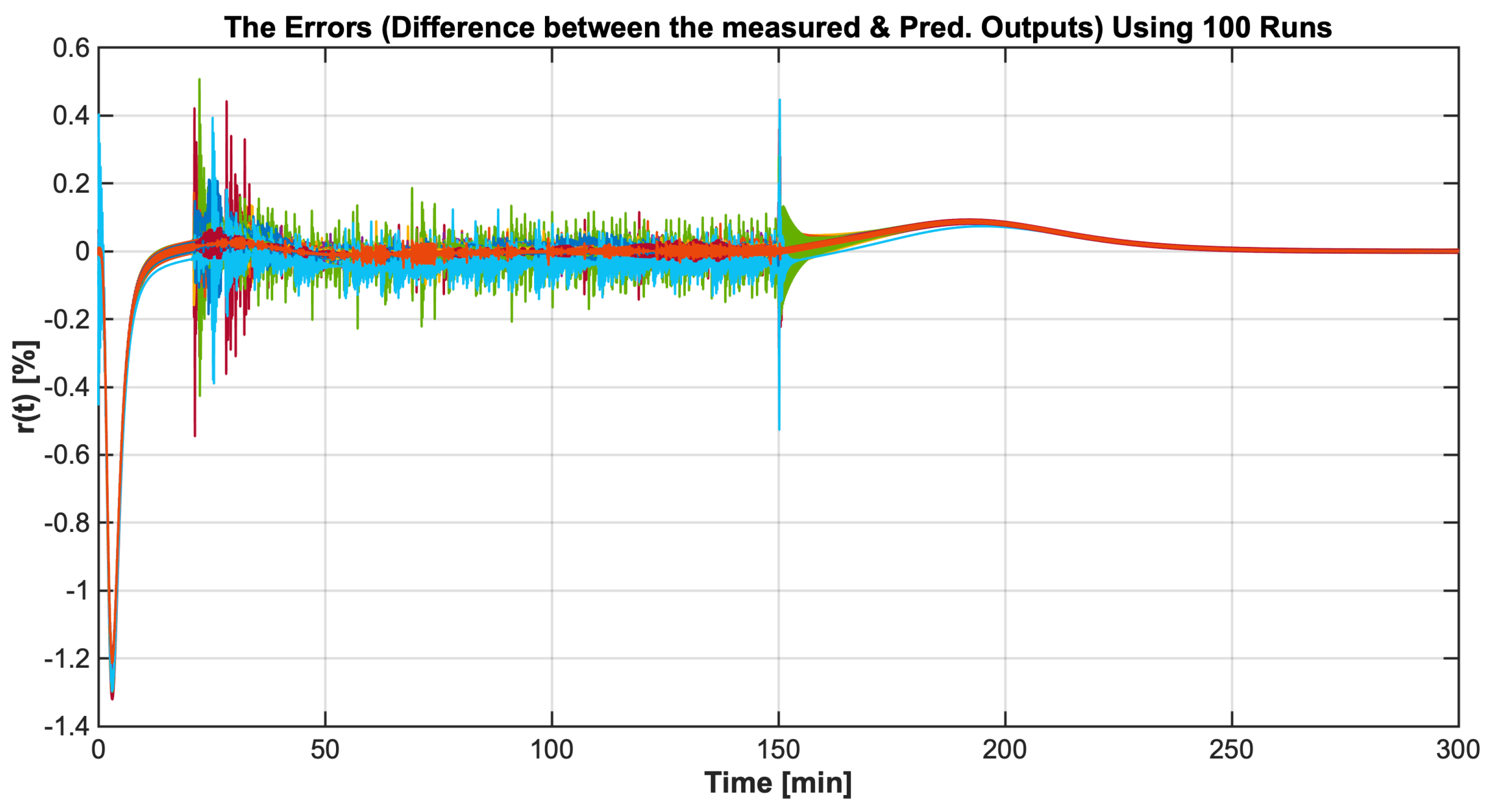
In addition, the percentage error or difference between measured and predicted output, in 100 runs, is shown in Figure 7. It is noticed that the errors are concentrated in the maintenance phase where drug infusion rate is non-zero and shows a lot of variations and changes, while in the recovery phase (after 150 min) the input is zero because drug injection is stopped, as shown in Figure 4. Nevertheless, the error is still very small and rarely exceeds %.
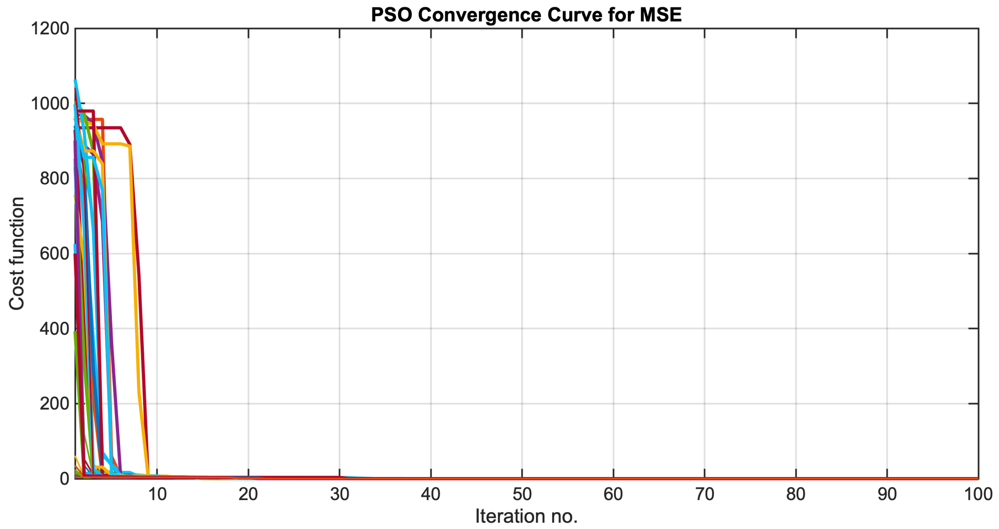
Finally, the convergence curves for the cost function during optimization using PSO algorithm are shown in Figure 8. It can been seen that the cost function converges to a minimum in less than 10 iterations.

5. Summary and Future Work

In this paper, the Wiener Box-Jenkins model is used successfully to predict the anesthesia level of the neuromuscular blockade (NMB) given the atracurium infusion rate. The model parameters are estimated using particle swarm optimization (PSO) in order to minimize the mean square error (MSE). The proposed approach showed very promising results with a convergence rate less than 15 iteration.
As a possible extension to the current work, instead of using simulated data, real data can be sought and used to test the proposed technique. Another possibility is to try to fine-tune the algorithm to achieve better accuracy or faster convergence.

Author Contributions

Conceptualization, I.A. and A.A.; Data curation, A.A.; Funding acquisition, I.A.; Methodology, I.A. and A.A.; Project administration, I.A.; Resources, I.A.; Software, A.A. and I.A.; Validation, I.A. and A.A.; Writing—review & editing, I.A. and A.A. All authors have read and agreed to the published version of the manuscript.

Funding

This research was funded by the Deanship of Scientific Research (DSR), Imam Abdulrahman Bin Faisal University, with a Grant No. 2020-110-Eng.

Institutional Review Board Statement

Not applicable.

Informed Consent Statement

Not applicable.

Data Availability Statement

Not applicable.

Acknowledgments

The authors would like to express their sincere gratitude to the anonymous reviewers for their valuable comments, which greatly improved the quality of the manuscript. The first author extends his appreciation to the Deanship of Scientific Research (DSR), Imam Abdulrahman Bin Faisal University for funding this research work through the project number No. 2020-110-Eng, and thanks the Biomedical Engineering Department, Imam Abdulrahman Bin Faisal for their continuous support. The second author would like to acknowledge the Department of Computer and Systems Engineering, Zagazig University, for their continuous support and encouragement.

Conflicts of Interest

The authors declare no conflict of interest.

References

  1. Butterworth, J.; Mackey, D.; Wasnick, J. The Anesthesia Machine. In Morgan & Mikhail’s Clinical Anesthesiology, 5th ed.; McGraw-Hill Education: New York, NY, USA, 2013; pp. 43–86. [Google Scholar]
  2. Guo, Z.; Medvedev, M.; Merigo, L.; Latronico, N.; Paltengh, M.; Visioli, A. Synthetic patient database of drug effect in general anesthesia for evaluation of estimation and control algorithms. In Proceedings of the 18th IFAC Symposium System Identification, Stockholm, Sweden, 9–11 July 2018; pp. 323–328. [Google Scholar]
  3. Dumont, G. Closed-loop control of anesthesia—A review. In Proceedings of the 8th IFAC Symposium on Biological and Medical Systems, Budapest, Hungary, 29–31 August 2012; pp. 373–375. [Google Scholar]
  4. Da Silva, M. System Identification and Control for General Anesthesia Based on Parsimonious Wiener Models. Licentiate Thesis, Division of Systems and Control, Uppsala University, Uppsala, Sweden, 2012. [Google Scholar]
  5. Soltesz, K.; Hahn, J.; Dumont, G.; Ansermino, J. Individualized PID control of depth of anesthesia based on patient model identification during the induction phase of anesthesia. In Proceedings of the 50th IEEE Conference Decision and Control, Orlando, FL, USA, 12–15 December 2011; pp. 855–860. [Google Scholar]
  6. Medvedev, A.; Zhusubaliyev, Z.; Rosén, O.; Silva, M. Oscillations-free PID control of anesthetic drug delivery in neuromuscular blockade. Comput. Methods Programs Biomed. 2019, 171, 119–131. [Google Scholar] [CrossRef] [PubMed]
  7. Costa, B.; Mendonça, T. GALENO: Computer aided system for modeling, monitoring, and control in anesthesia. Adv. Control Appl. Eng. Ind. Syst. 2021, 3, e87. [Google Scholar] [CrossRef]
  8. Hegedus, E.; Birs, I.; Muresan, C. Fractional Order Control of the Combined Anaesthesia-Hemodynamic System: A Preliminary Study. IFAC-PapersOnLine 2021, 54, 19–24. [Google Scholar] [CrossRef]
  9. Ionescu, C.M.; De Keyser, R.; Torrico, B.C.; De Smet, T.; Struys, M.M.; Normey-Rico, J.E. Robust predictive control strategy applied for propofol dosing using BIS as a controlled variable during anesthesia. IEEE Trans. Biomed. Eng. 2008, 55, 2161–2170. [Google Scholar] [CrossRef] [PubMed]
  10. Araujo, H.; Xiao, B.; Liu, C.; Zhao, Y.; Lam, H. Design of type-1 and interval type-2 fuzzy PID control for anesthesia using genetic algorithms. J. Intell. Learn. Syst. Appl. 2014, 4, 70–93. [Google Scholar] [CrossRef] [Green Version]
  11. Jaklitsch, R.; Westenskow, D. A model-based self-adjusting two-phase controller for vecuronium-induced muscle relaxation during anesthesia. IEEE Trans. Biomed. Eng. 1987, 38, 583–594. [Google Scholar] [CrossRef] [PubMed]
  12. Kudva, H.; Warrier, J. Automated anesthesia delivery pump. IOSR J. Pharm. Biol. Sci. 2014, 9, 100–106. [Google Scholar] [CrossRef]
  13. Haddad, W.; Volyanskyy, K.; Bailey, J. Neuroadaptive output feedback control for automated anesthesia with noisy EEG measurements. IEEE Trans. Control Syst. Technol. 2011, 19, 311–326. [Google Scholar] [CrossRef]
  14. Soltesz, K.; Heusden, K.; Hast, M.; Ansermino, J.; Dumont, G. A synthesis method for automatic handling of inter-patient variability in closed-loop anesthesia. In Proceedings of the American Control Conference (ACC), Boston, MA, USA, 6–8 July 2016; pp. 4877–4882. [Google Scholar]
  15. Bibian, S.; Ries, C.; Huzmezan, M.; Dumont, G. Clinical anesthesia and control engineering: Terminology, concepts and issues. In Proceedings of the European Control Conference (ECC), Cambridge, UK, 1–4 September 2003; pp. 2430–2439. [Google Scholar] [CrossRef]
  16. Hahn, J.; Dumont, G.; Ansermino, J. A direct dynamic dose-response model of propofol for individualized anesthesia care. IEEE Trans. Biomed. Eng. 2012, 59, 571–578. [Google Scholar] [CrossRef] [PubMed]
  17. Brouse, C.; Karlen, W.; Dumont, G.; Myers, D.; Cooke, E.; Stinson, J.; Lim, J.; Ansermino, J. Real-time cardiorespiratory coherence detects antinociception during general anesthesia. In Proceedings of the 34th Annual International Conference IEEE EMBS, San Diego, CA, USA, 28 August–1 September 2012; pp. 3813–3816. [Google Scholar]
  18. Heusden, K.; Ansermino, J.; Dumont, G. Closed-loop instrumental variable identification of propofol anesthesia. In Proceedings of the IEEE Conference on Control Technology and Applications (CCTA), Mauna Lani Resort, HI, USA, 27–30 August 2017; pp. 1165–1170. [Google Scholar]
  19. Dumont, G.; Martinez, A.; Ansermino, J. Robust control of depth of anesthesia. Int. J. Adapt. Control Signal Process. 2008, 23, 435–454. [Google Scholar] [CrossRef]
  20. Ionescu, C.M.; Copot, D.; Neckebroek, M.; Muresan, C. Anesthesia regulation: Towards completing the picture. In Proceedings of the IEEE International Conference Automation, Quality and Testing, Robotics (AQTR), Cluj-Napoca, Romania, 24–26 May 2018; pp. 1–6. [Google Scholar]
  21. Da Silva, M.; Wigrn, T.; Mendonca, T. Nonlinear identification of a minimal neuromuscular blockade model in anesthesia. IEEE Trans. Control Syst. Technol. 2012, 20, 181–188. [Google Scholar] [CrossRef]
  22. Da Silva, M. Prediction error identification of minimally parameterized Wiener models in anesthesia. In Proceedings of the 18th IFAC World Congress, Milan, Italy, 28 August–2 September 2011; pp. 5615–5620. [Google Scholar]
  23. Heusden, K.; Dumont, G.; Soltesz, K.; Petersen, C.; Umedaly, A.; West, N.; Ansermino, J. Design and clinical evaluation of robust PID control of propofol anesthesia in children. IEEE Trans. Control Syst. Technol. 2014, 22, 491–501. [Google Scholar] [CrossRef] [Green Version]
  24. van Heusden, K.; Ansermino, J.; Soltesz, K.; Khosravi, S.; West, N.; Dumont, G. Quantification of the variability in response to propofol administration in children. IEEE Trans. Biomed. Eng. 2013, 60, 2521–2529. [Google Scholar] [CrossRef] [PubMed] [Green Version]
  25. Silva, M.; Mendonca, T.; Wigren, T. On-line nonlinear identification of the effect of drugs in anaesthesia using a minimal parameterization and BIS measurements. In Proceedings of the American Control Conference, Baltimore, MD, USA, 30 June–2 July 2010; pp. 4379–4384. [Google Scholar]
  26. Eberhart, R.; Kennedy, J. A new optimizer using particle swarm theory. In Proceedings of the 6th International Symposium on Micro Machine and Human Science, Nagoya, Japan, 4–6 October 1995; pp. 39–43. [Google Scholar]
  27. Pal, P.; Dasgupta, A.; Akhil, J.; Kar, R.; Mandal, D.; Ghosal, S. Identification of a Box-Jenkins structured two stage cascaded model using simplex particle swarm optimization algorithm. In Proceedings of the 2016 International Symposium on Intelligent Signal Processing and Communication Systems, Phuket, Thailand, 24–27 October 2016; pp. 1–4. [Google Scholar]
  28. Montain, M.; Blanco, A.; Bandoni, J. Optimal drug infusion profiles using a particle swarm optimization algorithm. Comput. Chem. Eng. 2015, 82, 13–24. [Google Scholar] [CrossRef]
  29. Alonso, H.; Mendonca, T.; Rocha, P. A hybrid method for parameter estimation and its application to biomedical systems. Comput. Methods Programs Biomed. 2008, 89, 112–122. [Google Scholar] [CrossRef] [PubMed]
  30. Ljung, L. System Identification: Theory for the User, 2nd ed.; Prentice Hall PTR: Hoboken, NJ, USA, 1999. [Google Scholar]
  31. Pintelon, R.; Schoukens, J. System Identification: A Frequency Domain Approach, 2nd ed.; Wiley-IEEE Press: New York, NY, USA, 2012. [Google Scholar]
  32. Aljamaan, I.; Westwick, D.; Foley, M. Non-iterative identification of IIR Wiener systems using orthogonal polynomial. In Proceedings of the 17th IFAC World Congress Conference, Cape Town, South Africa, 24–29 August 2014; Volume 47, pp. 487–492. [Google Scholar]
  33. Dempsey, E.; Westwick, D. Identification of Hammerstein models with cubic spline nonlinearities. IEEE Trans. Biomed. Eng. 2004, 51, 237–245. [Google Scholar] [CrossRef] [PubMed]
  34. Aljamaan, I.; Bshait, B.; Westwick, D. Separable least squares identification of Wiener Box-Jenkins models. In Proceedings of the 18th IFAC World Congress, Milan, Italy, 28 August–2 September 2011; Volume 18, pp. 4434–4439. [Google Scholar]
  35. Bonyadi, M.; Michalewicz, Z. Particle swarm optimization for single objective continuous space problems: A review. Evol. Comput. 2017, 25, 1–54. [Google Scholar] [CrossRef] [PubMed]
  36. Wang, D.; Tan, D.; Liu, L. Particle swarm optimization algorithm: An overview. Soft Comput. 2018, 22, 387–408. [Google Scholar] [CrossRef]
  37. Merigo, L.; Padula, F.; Latronico, N.; Mendonca, T.; Paltenghi, M.; Rocha, P.; Visioli, A. Optimized PID tuning for the automatic control of neuromuscular blockade. In Proceedings of the 3rd IFAC Conference on Advances in Control PID, Ghent, Belgium, 9–11 May 2018; Volume 51, pp. 66–71. [Google Scholar]
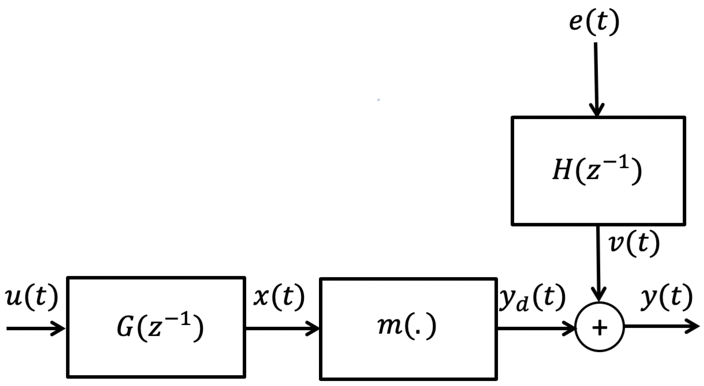
Figure 1. The proposed Wiener Box-Jenkins model structure.
Applsci 12 04817 g001
Figure 2. Flowchart of the PSO optimization algorithm.
Applsci 12 04817 g002
Figure 3. SIMULINK model for the closed-loop administration of atracurium.
Applsci 12 04817 g003
Figure 4. The atracurium infusion rate, u ( t ) , the level of neuromuscular blockade (NMB), and the set point, r ( t ) , in a sample run.
Applsci 12 04817 g004
Figure 5. Average measured and predicted NMB outputs over 100 Monte Carlo simulations.
Applsci 12 04817 g005
Figure 6. The predicted ouptut in 100 Monte Carlo runs using the proposed PSO-based Wiener Box-Jenkins identification approach.
Applsci 12 04817 g006
Figure 7. The difference between the measured and estimated output using 100 Monte Carlo runs using the proposed PSO method.
Applsci 12 04817 g007
Figure 8. Convergence curves for the MSE cost function in 100 Monte Carlo runs.
Applsci 12 04817 g008
Table 1. Parameters of the PSO algorithm.
ParameterValue
Population size, N p 50
θ m i n −2
θ m a x +2
Inertia coefficient, w 1.0
Damping ratio of inertia coefficient, ζ d a m p 0.9
Personal acceleration coefficient, c 1 2.0
Social acceleration coefficient, c 2 2.0
Maximum iterations00
Table 2. Simulation settings for PID controller gains and parameters of patient number 17.
ParameterValue
PID controller K P 64.9721
K I 17.5456
K D 6.3897
Patient C ¯ 50 γ 3.2425
λ 0.3
α 0.0366
γ 1.9262
k 1 1
k 2 2
k 3 10
Table 3. Average estimates of the Wiener Box-Jenkins model parameters using PSO.
ParameterValue
b 0 0.0085
b 1 0.0028
b 2 0.0020
f 1 0.0261
f 2 0.1744
c 1 0.9926
d 1 1.0000
β 0 100.0063
β 1 0.0703
β 2 0.0054
β 3 0.0445
Table 4. Mean square error (MSE), % Variance Accounted for, Mean Absolute Error (MAE), Mean Absolute Percentage Error (MAPE) and R 2 averaged over 100 Monte Carlo simulations.
MSE % VAR MAEMAPE R 2
0.0127 99.9 % 0.0331 0.0010 0.9997
Publisher’s Note: MDPI stays neutral with regard to jurisdictional claims in published maps and institutional affiliations.