Wind Turbine Fault Diagnosis by the Approach of SCADA Alarms Analysis

Featured Application

The research proposed in this paper could be useful in wind turbine condition monitoring and fault diagnosis.

Abstract

Wind farm operators are overwhelmed by a large amount of supervisory control and data acquisition (SCADA) alarms when faults occur. This paper presents an online root fault identification method for SCADA alarms to assist operators in wind turbine fault diagnosis. The proposed method is based on the similarity analysis between an unknown alarm vector and the feature vectors of known faults. The alarm vector is obtained from segmented alarm lists, which are filtered and simplified. The feature vector, which is a unique signature representing the occurrence of a fault, is extracted from the alarm lists belonging to the same fault. To mine the coupling correspondence between alarms and faults, we define the weights of the alarms in each fault. The similarities is measured by the weighted Euclidean distance and the weighted Hamming distance, respectively. One year of SCADA alarms and maintenance records are used to verify the proposed method. The results show that the performance of the weighted Hamming distance is better than that of the weighted Euclidean distance; 84.1% of alarm lists are labeled with the right root fault.

1. Introduction

As wind power installations continue worldwide, wind power is in a rapid transition toward becoming a fully commercialized, unsubsidized technology. It is thus vital to reduce the levelized wind power energy cost for enhancing the competitiveness of wind farms during the transition to fully commercial, market-based operations. Due to the remote and harsh operational environment, the operation and maintenance (O&M) costs of wind farms are high. Statistics show that the O&M costs account for 10–15% of total wind farm project costs [1]. For an offshore wind farm, the O&M costs account for up to 14–30% [2]. To reduce O&M costs, it is necessary to improve the reliability of wind turbines. Therefore, condition monitoring and fault diagnosis methods are commonly developed and employed [3].

Supervisory control and data acquisition (SCADA) systems are a standard installation for large wind turbines, and provide a wide range of operational information for almost all the subcomponents. As a potentially low-cost and wide-coverage solution, plentiful studies using SCADA data for condition monitoring and fault diagnosis were developed [4,5]. Moreover, the SCADA system also provides alarms to operators when a process key variable crosses a pre-fixed threshold, or a fault of a subcomponent occurs. These alarms can be used as emergency event indicators that assist operators in mitigating risk. However, these SCADA alarms are often overlooked in industrial applications for the following reasons: (1) The occurrence of a fault usually raises alarm floods. An alarm flood refers to a situation during which tens or hundreds of alarms appear in a short time [6]. The operator is overwhelmed by these alarm floods because it exceeds his response capability. (2) Because of the bad alarm configuration and the causal relationships among the measured variables, a large proportion of alarms are nuisance alarms, such as chattering alarms [7] and other related alarms [8]. It is difficult for the operator to respond to the critical alarms promptly due to the presence of these nuisance alarms. (3) Alarms typically contain descriptive information about an abnormal situation. The operator cannot find the root cause of a fault directly through SCADA alarms. When overwhelmed by alarms, the operator needs to rely on extra expert consultation. This paper aims to solve the above problems existing in wind turbine SCADA alarms and assist the operator in wind-turbine fault diagnosis.

Some researchers focused on the use of SCADA alarms for the fault diagnosis of wind turbines. A time sequence method and probability-based method were proposed in [9] for analyzing SCADA alarms. The fault cases on the wind turbine converter and pitch system were used to verify the proposed methods. The results showed that both methods had the potential to rationalize alarm data and identify fault locations. However, the issue of time consumption must be solved when the methods are applied to larger data. A study of wind turbine alarm processing and diagnosis using an artificial neural network was proposed in [10]. The alarm behaviors were transformed into an alarm matrix, which was obtained by inputting the data for each fault into an alarm vector. Each vector represented the alarm pattern of one pitch system fault. The repetitive occurrence of alarm patterns was not studied in depth. Reference [11] used an improved Apriori algorithm to analyze the alarms, which occurred during blade angle asymmetry faulta. The results showed that the related alarms could be integrated into one critical alarm to reduce the number of alarms. The accuracy of the method is limited due to its dependence on sufficient sample data. A method for identifying relevant alarms and grouping similar alarm sequences was presented in [12]. Similar alarm sequences were grouped using clustering techniques. However, the used cluster algorithms did not perform as well as hoped.

The issue of a large number of alarms not only exists in the wind power domain but in many other domains, such as network management [13], IT security [14], and process control in manufacturing systems [15]. Researchers and vendors proposed many approaches to alarm reduction and correlation [16]. A similarity analysis is one of the most common methods used in analyzing alarms. It aims to reduce the total number of alarms by aggregating them using their similarities. This strategy is based on the assumption that similar alarms tend to have the same root causes. The key step in a similarity analysis is to define appropriate similarity measures.

An analysis method was proposed in [17] to investigate similar alarm floods from historic alarms. The dissimilarity score between each pair of alarm floods was calculated using the Jaccard distance. The similar floods were clustered into groups using the Agglomerative Hierarchical Clustering algorithm. The results showed that the grouping of alarm floods could be used to eliminate sequential alarms and ascertain rationalization suggestions. An online algorithm was proposed in [18] to provide an early prediction of an incoming alarm flood. The alarm sequences were clustered into similar groups based on their similarity scores. A pattern database of the common patterns was formed for each cluster. The online alarm sequence was matched with these patterns. A method to extract a fault template from a set of alarm lists, raised on the occurrence of several faults, was proposed in [19,20]. The fault template could be used to extract relevant information on the alarm system and by operators as a guideline for fault diagnosis. The proposed fault isolation method was based on a weighted sequential similarity measure.

Motivated by the shortcomings of the existing methods in the wind power domain, this paper proposes an online fault diagnosis method for SCADA alarms based on a similarity analysis. The proposed method does not require a time-consuming training procedure and is accessed via an easy online application. Moreover, it is not over-reliant on the available data. As the data increase, the performance of the proposed method becomes self-optimizing. Our main contributions are as follows:

• We segment alarms into alarm lists by an information alarm and represent alarm lists by vectors to simplify alarms;
• We extract the feature vector from alarm vectors as a unique signature representing an occurring fault;
• We define the weights of alarms to establish the coupling correspondence between alarms and faults.

The remainder of this paper is organized as follows: Section 2 introduces SCADA alarms and maintenance logs; Section 3 presents the online root fault identification method; Section 4 presents the results and the discussion; and Section 5 presents the conclusions.

2. Background

2.1. SCADA Alarms

Alarm systems [21] play an important role in process monitoring. Due to advanced technologies, modern wind turbines use hundreds of sensors and actuators as parts of their many control loops. This situation can result in a large number of measured variables and their corresponding configured alarms. Thus, alarms can be generated at a high rate. A wind turbine SCADA system is integrated with an alarm function, which monitors the condition of wind turbines and their subcomponents.

Alarms are stored in the SCADA database. A list of the alarms used in this paper is shown in

Table 1. A list of SCADA alarms.

Turbine Number	Time	Type	Code	Flag	Description
P01	2017/5/22 16:30:05	information	I2	start	The wind turbine is started
P01	2017/5/22 17:38:18	warning	A264	start	The first measuring point temperature of the generator stator is high
P01	2017/5/22 17:38:37	warning	A264	end	The first measuring point temperature of the generator stator is high
P01	2017/5/22 17:38:51	fault	T21	start	The communication of the pitch system is an error
P01	2017/5/22 17:38:52	information	I2	end	The wind turbine is started
P01	2017/5/23 00:15:20	fault	T21	end	The communication of the pitch system is an error

. They are recorded in chronological order. There are three types of alarms: information alarms, warning alarms, and fault alarms. Information alarms are generally used to communicate changes in certain operating conditions, e.g., wind turbine is reset, or a manual switch is engaged. Warning alarms are generated when the monitored variables come close to exceeding thresholds. Fault alarms are generated when these thresholds are exceeded. The attribute ‘code’ is the unique code of an alarm. The attribute ‘flag’ represents the start and the end of each alarm. Hence, each alarm has two records.

2.2. Maintenance Log

The maintenance log collects the repair activities carried out by the maintenance engineers. A record of this is shown in

Table 2. An example of a record in maintenance log.

Turbine Number	Start Time	End Time	Subcomponents	Types of Faults	Solutions	Downtime/h
1	2016/12/21 17:34:00	2016/12/25 12:45:00	Pitch system	Slip ring is damaged	Replace the slip ring	91.18

. The attribute ‘type of faults’ reveals the actual fault of this repair activity. It is the root fault of the corresponding alarms.

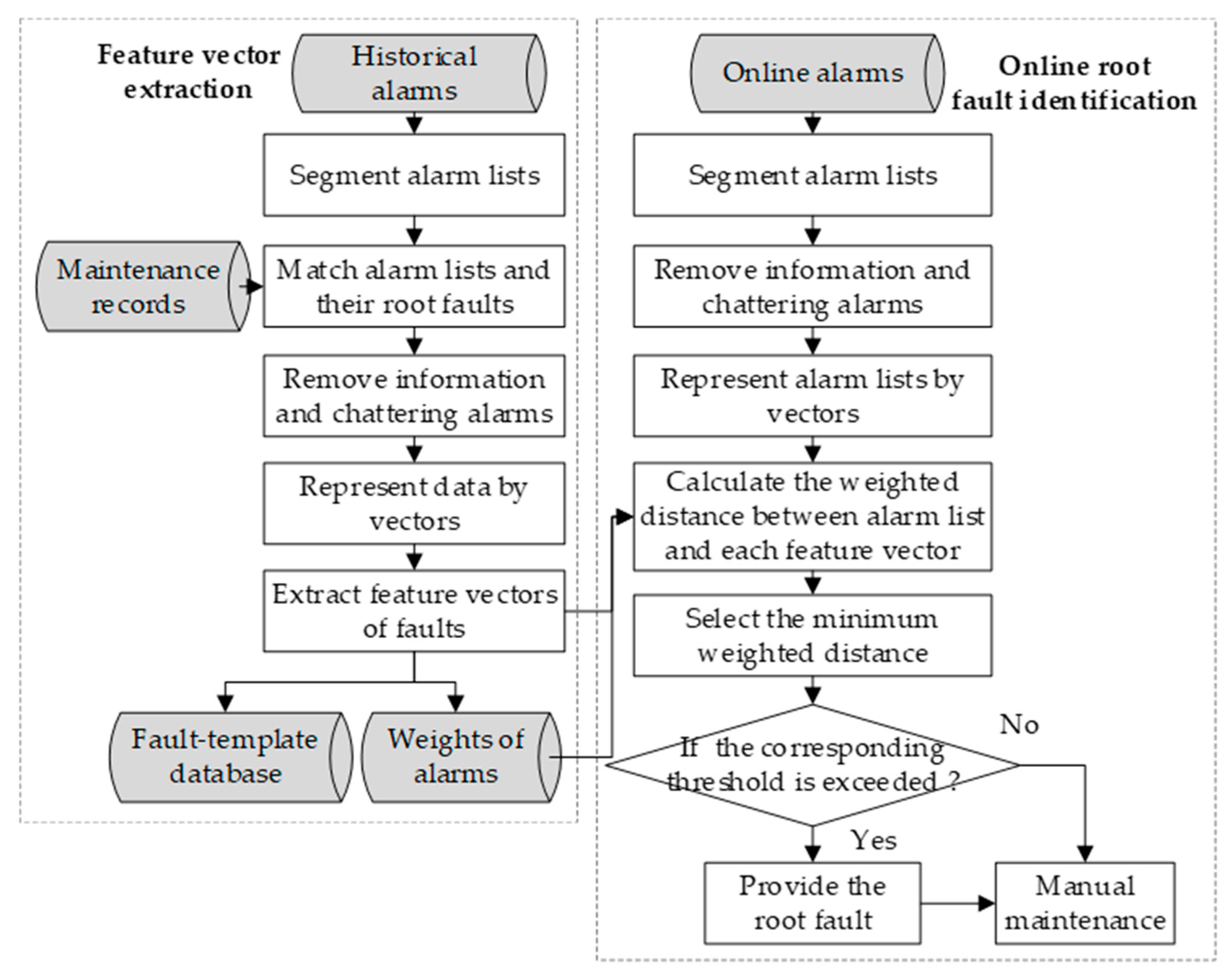
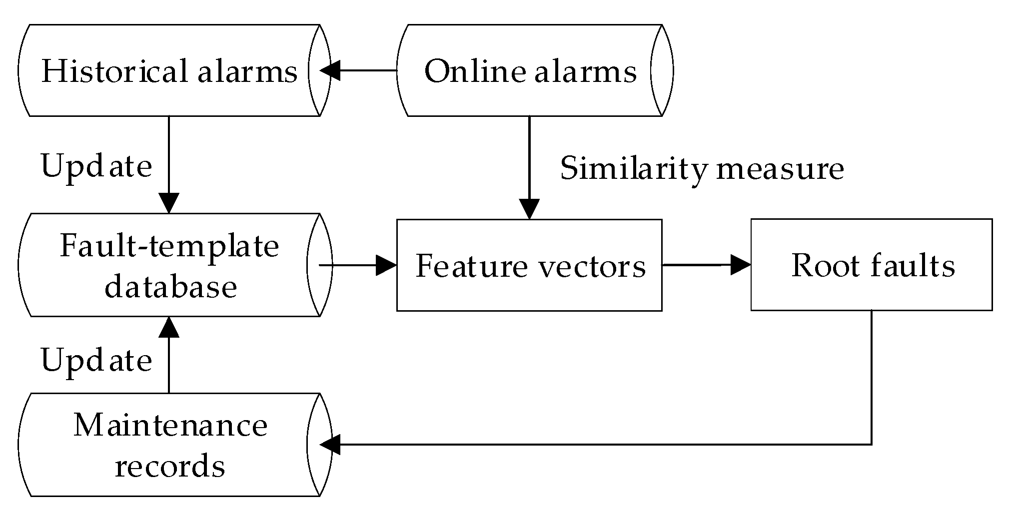
3. Online Root Fault Identification Method

This study proposes an online root fault identification method based on a similarity analysis. The idea of the method is based on the assumption that similar alarms tend to have the same root faults. The flowchart of the proposed method is shown in Figure 1. There are two processes: feature vector extraction and online root fault identification. Briefly, in the process of feature vector extraction, alarms are firstly segmented into alarm lists, and the information and chattering alarms are removed. Subsequently, the alarm lists and their root faults are matched. Finally, the feature vectors of faults are extracted and the fault-template database is built. To establish the coupling correspondence between an alarm and a fault, the weight of an alarm in a fault is defined. In the process of online fault identification, firstly, the online alarms are preprocessed and represented by vectors. Afterward, the weighted distance between an online alarm vector and the feature vectors is calculated. The root fault of the online alarm vector is deduced by the value of similarity.

3.1. Feature Vector Extraction

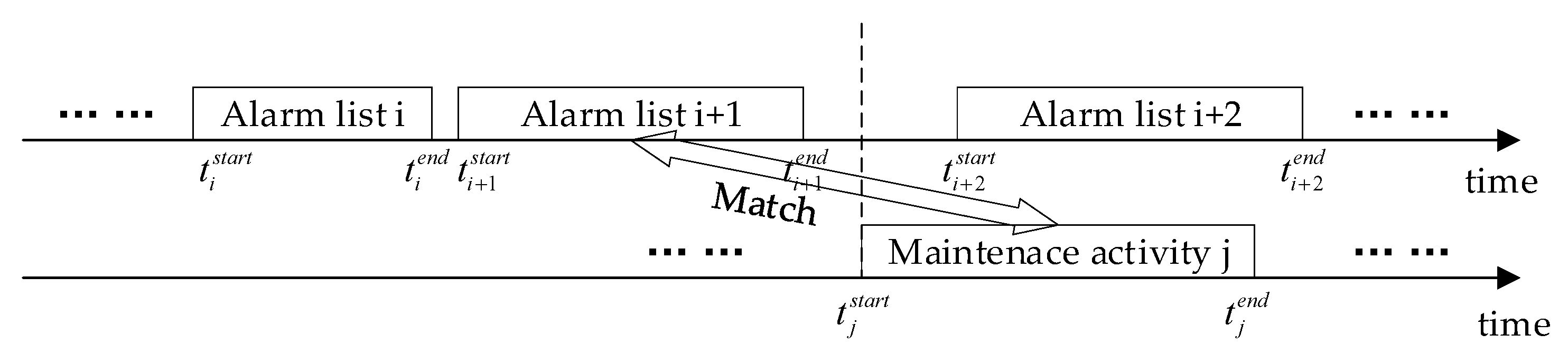
3.1.1. Segmenting Alarm Lists

The alarms are recorded continuously in chronological order. First of all, we need to segment continuous alarms into alarm lists. The information alarm, ‘I2’ is used to segment alarm lists in this paper.

A SCADA system not only monitors process variables and triggers alarms, but also changes the operating condition of a wind turbine to deal with alarms. The actions in response to alarms are different according to the alarm levels. When the alarm level is low, no operation is performed, or the wind turbine is restarted to try to eliminate alarms. On the contrary, when the alarm level is high, the wind turbine is shut down, awaiting manual maintenance. Therefore, every time one wind turbine is shut down due to a fault, it needs manual maintenance.

The information alarm ‘I2’ indicates that the wind turbine is started. When the flag of I2 is ‘start’, the wind turbine is started from a shutdown. When the flag of I2 is ‘end’, the wind turbine is shut down from running; that is to say, the start of I2 indicates that the wind turbine has returned to normal operation, and the end of I2 indicates that the wind turbine is shut down due to faults. All the alarms generated between the start of I2 and the end of I2 are related to the following shutdown. Therefore, we segment alarms into alarm lists using I2. The alarms generated between the start of I2 and the end of I2 make an alarm list. The total number of alarm lists is expressed as M.

3.1.2. Matching Alarm Lists and Their Root Faults

Every time one wind turbine is shut down due to a fault, manual maintenance is needed. Therefore, the root fault of each alarm list is recorded in the maintenance log. The total number of records is Q. In theory, Q should be equal to the total number of alarm lists M. However, Q is smaller than M. This is due to the irregular work of operators in the industry. Some maintenance activities are missing.

The end time of alarm lists and the start time of maintenance activities is used to match alarm lists and their root faults. The schematic diagram of the match criterion is shown in Figure 2. The end time of an alarm list should be earlier than the start time of maintenance activity. The alarm list corresponding to the maintenance activity is the last list. Ultimately, we obtain Q pairs of data, which are made up of alarm lists and their root faults.

3.1.3. Removing Information and Chattering Alarms

The information alarms generally communicate changes in the operating conditions of wind turbines. We are not interested in such alarms. We focus on the warning alarms and fault alarms that indicate the abnormalities of the wind turbine. Thus, the information alarms are removed.

A chattering alarm [22] is an alarm that appears repeatedly during a short time. The reasons for a chattering alarm are that the monitored process variable is close to the alarm threshold and a noise is present. In this paper, we keep the first alarm of the chattering alarms in one alarm list and remove the following repeated alarms.

3.1.4. Representing Data by Vectors

The occurrence of an alarm can be recorded as a binary value. If the alarm is present, the value is equal to one; if the alarm is not present, the value is equal to zero. The binary value is expressed as:

$$v_i=\{\begin{array}{c}1, \mathrm{if} \mathrm{alarm} i \mathrm{is} \mathrm{present} \\ 0, \mathrm{if} \mathrm{alarm} i \mathrm{is} \mathrm{not} \mathrm{present}\end{array},$$

(1)

where $i=1,2,\dots ,N$ and N is the total number of alarm types configured in the SCADA system.

A list of alarms may be represented either by a sequence of alarms or by a vector of alarms. In a sequence, the alarms are ordered by their time of appearance. In a vector, their time of appearance is not considered. Only the fact that the alarms are present is considered. In this paper, an alarm list is represented by a vector. The j-th alarm vector is expressed as:

$$V^j={[v_1^j,v_2^j,\dots ,v_i^j,\dots ,v_N^j]}^{\mathrm{T}},$$

(2)

where $v_i^j$ is the binary value of alarm i in the j-th alarm vector; $j=1,2,\dots ,M$; M is the total number of alarm vectors. It should be noted that each alarm has two records: one record represents the start of the alarm; another record represents the end of the alarm. In an alarm vector, as long as one alarm occurs, the binary value of the alarm is set to one.

Fault k in the r-th maintenance record is expressed as:

$$f_k^r(r=1,2,\dots ,Q,k=1,2,\dots ,P),$$

(3)

where Q is the total number of maintenance records and P is the number of fault types. Because the same fault can happen multiple times, P is smaller than Q. All the faults in records are expressed as:

$$F=\{f_1^1,f_1^2,\dots ,f_1^{l_1},\dots ,f_k^1,f_k^2\dots ,f_k^{l_k},\dots ,f_P^{l_P}\},$$

(4)

where $f_k^{l_k}$ is fault k in the $l_k-\mathrm{th}$ maintenance record; $l_k$ is the number of records belonging to fault k; and $l_P$ is the number of records belonging to fault P. Thus, the set of records belonging to fault k is expressed as:

$$F_k=\{f_k^1,f_k^2,\dots ,f_k^{l_k}\},$$

(5)

where $f_k^{l_k}$ is fault k in the $l_k-\mathrm{th}$ maintenance record; $l_k$ is the number of records belonging to fault k; $k=1,2,\dots ,P$. Thus, ${\displaystyle \sum _{k=1}^P{l}^k}=Q$.

After the match process, the alarm vectors are labeled with their root faults. The pairs of alarm vectors and their root faults are expressed as:

$$\{(V_k^1,f_k^1),(V_k^2,f_k^2),\dots ,(V_k^{l_k},f_k^{l_k})\},$$

(6)

where $V_k^{l_k}$ is the $l_k-\mathrm{th}$ alarm vector of fault k; $f_k^{l_k}$ is fault k in the $l_k-\mathrm{th}$ maintenance record; $k=1,2,\dots ,P$.

3.1.5. Feature Vector Extraction

The same fault of the wind turbine can happen multiple times. However, the alarm lists generated during the same fault are not always the same, since the physical processes are not deterministic, and the environmental conditions may differ when a fault occurs. This section aims to extract the feature vector of alarm vectors belonging to the same fault. The feature vector is used as a unique signature representing the occurrence of a fault.

There are $l_k$ alarm lists generated when fault k occurs. The alarm vector belonging to fault k is expressed as:

$$V_k^j={[v_{k1}^j,v_{k2}^j,\dots ,v_{ki}^j,\dots ,v_{kN}^j]}^{\mathrm{T}},$$

(7)

where $v_{ki}^j$ is the binary value of alarm i in the j-th alarm vector of fault k; $j=1,2,\dots ,l_k$. The feature vector of fault k is expressed as:

$$C_k={[c_{k1},c_{k2},\dots ,c_{ki},\dots ,c_{kN}]}^{\mathrm{T}},$$

(8)

where $c_{ki}$ is the binary value of alarm i in fault k; $k=1,2,\dots ,P$; and P is the number of fault types. The feature vector $C_k$ is built using the $l_k$ alarm vectors belonging to fault k. The binary value of alarm i in the alarm vector of fault k is calculated as follows:

$$c_{ki}=\{\begin{array}{c}1, \mathrm{if}\frac{{\displaystyle \sum _{j=1}^{l_k}{v}_{ki}^j}}{l_k}\ge fr\\ 0, \mathrm{if}\frac{{\displaystyle \sum _{j=1}^{l_k}{v}_{ki}^j}}{l_k}<fr\end{array},$$

(9)

where $v_{ki}^j$ is the binary value of alarm i in the j-th alarm vector of fault k; and $fr\in [0,1]$ is a frequency. If alarm i is frequently triggered by fault k, the corresponding alarm in the feature vector is set to one; otherwise, it is set to zero. The value of fr is set to 0.5 in this paper. It is determined according to the final performance.

A pair of a fault and its feature vector is expressed as:

$$(f_k,C_k),$$

(10)

where $f_k$ is fault k; $C_k$ is the feature vector of fault k; and $k=1,2,\dots ,P$. The fault-template database is composed of faults and their feature vectors. It is expressed as:

$$T=\{(f_1,C_1),(f_2,C_2),\dots ,(f_k,C_k),\dots ,(f_p,C_p)\},$$

(11)

where $f_k$ is fault k; $C_k$ is the feature vector of fault k; and $k=1,2,\dots ,P$.

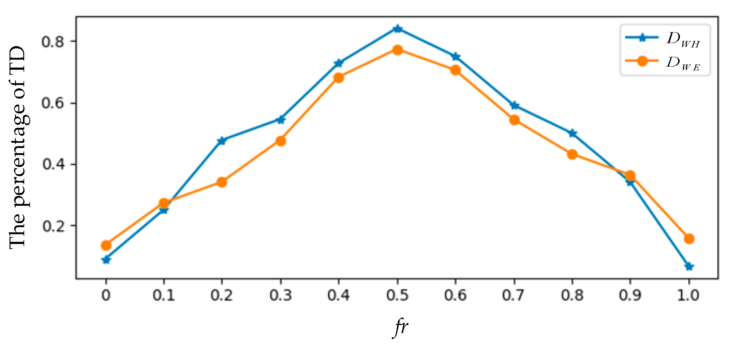
3.1.6. Weights of Alarms

When a fault occurs, the responses from alarms are different. To explore the coupling correspondence between alarms and faults, we define the weights of alarms in each fault. The weight of alarm i in fault k is expressed as:

$$w_{ki}={\lambda }_{1i}{\lambda }_{2ki}{\lambda }_{3ki},(k=1,2,\dots ,P;i=1,2,\dots ,N),$$

(12)

where ${\lambda }_{1i}$ is the weight defined according to the alarm type; ${\lambda }_{2ki}$ is the weight defined according to the significance of alarm i in fault k; ${\lambda }_{3ki}$ is the weight defined according to the specificity of alarm i in fault k; P is the number of fault types; and N is the number of alarm types configured in the SCADA system.

• Alarm type

Warning alarms and fault alarms play different roles in the SCADA system. Warning alarms are triggered when the monitored variables come close to exceeding thresholds. Fault alarms are triggered when these thresholds are exceeded. Thus, fault alarms are more important than warning alarms. We define that the weights of fault alarms are bigger than those of warning alarms. The value of ${\lambda }_{1i}$ is determined as follows:

$${\lambda }_{1i}=\{\begin{array}{c}0.5, \mathrm{if} \mathrm{alarm} i \mathrm{is} \mathrm{a} \mathrm{warning} \mathrm{alarm}\\ 1.0, \mathrm{if} \mathrm{alarm} i \mathrm{is} \mathrm{a} \mathrm{fault} \mathrm{alarm} \end{array}.$$

(13)

2.

The significance of an alarm

When fault k occurs, some alarms are always triggered or never triggered. The indicative effect of these alarms in fault k is strong. Thus, the significance of these alarms is great. On the contrary, when fault k occurs, other alarms are not always triggered. The indicative effectiveness of these alarms in fault k is weak. Thus, these alarms have little significance. The weight ${\lambda }_{2ki}$ is used to enhance the alarms which are significant to one fault and discards the nonsignificant ones; ${\lambda }_{2ki}$ is calculated as follows:

$${\lambda }_{2ki}=2{\alpha }_{ki}-1,$$

(14)

$${\alpha }_{ki}=\frac{1}{l_k}{\displaystyle \sum _{j=1}^{l_k}\delta (v_{ki}^j-c_{ki})},$$

(15)

$$\delta (x)=\{\begin{array}{c}1, \mathrm{if} x=0\\ 0, \mathrm{if} x\ne 0\end{array},$$

(16)

where $v_{ki}^j$ is the binary value of alarm i in the j-th alarm vector of fault k; $c_{ki}$ is the binary value of alarm i in the alarm vector of fault k; $k=1,2,\dots ,P$; $i=1,2,\dots ,N$; P is the number of fault types; and N is the number of alarm types configured in the SCADA system.

When alarm i is always triggered or never triggered by fault k, ${\alpha }_{ki}=1$. When alarm i is triggered randomly, ${\alpha }_{ki}=0.5$. Therefore, ${\lambda }_{2ki}\in [0,1]$.

3.

The specificity of an alarm

When an alarm is only significant to fault k and nonsignificant to other faults, we consider that the alarm is unique to fault k. The weight ${\lambda }_{3ki}$ is used to enhance the alarms which are unique to fault k; ${\lambda }_{3ki}$ is calculated as follows:

$${\lambda }_{3ki}=1-\frac{1}{P-1}{\displaystyle \sum _{g\in F_{\overline{k}}}(\frac{1}{l_g}{\displaystyle \sum _{j=1}^{l_g}\delta (v_{gi}^j-c_{ki})})},$$

(17)

$$\delta (x)=\{\begin{array}{c}1, \mathrm{if} x=0\\ 0, \mathrm{if} x\ne 0\end{array},$$

(18)

where P is the number of faults, $F_{\overline{k}}$ is a finite set of faults except fault k, $v_{gi}^j$ is the binary value of alarm i in the j-th alarm vector of fault g; $c_{ki}$ is the binary value of alarm i in the alarm vector of fault k; $l_g$ is the number of alarm lists belonging to fault g.

The weight ${\lambda }_{3ki}$ decreases in the following situations: (1) Alarm i is frequently triggered by fault k and frequently triggered by the other faults. (2) Alarm i is seldom triggered by fault k or by the other faults. Therefore, ${\lambda }_{3ki}$ decreases when alarm i is shared by several faults, but increases when alarm i is more specific to fault k than to the other faults. The value range of ${\lambda }_{3ki}$ is between zero and one.

3.2. Online Root Fault Diagnosis

The first three steps in the process of online root fault identification are the same as those in the process of feature vector extraction.

3.2.1. Weighted Distance Calculation

• Distance measure

This similarity is typically measured by computing certain metrics. When compared with thresholds, the resulting score determines if one alarm vector belongs to a root fault. Choosing a suitable distance measure increases the overall performance of the online diagnosis. An online unknown alarm vector $V^{\prime }$ is expressed as:

$$V^{\prime }={[{v^{\prime }}_1,{v^{\prime }}_2,\dots {v^{\prime }}_i,\dots ,{v^{\prime }}_N]}^{\mathrm{T}}.$$

(19)

where ${v^{\prime }}_i$ is the binary value of alarm i. The distance between the alarm vector and the feature vector of fault k is expressed as:

$$D(V^{\prime },C_k),$$

(20)

where $C_k$ is the feature vector of fault k and $k=1,2,\dots ,P$.

The Euclidean distance [23] and the Hamming distance [24] are often used as metrics. The Euclidean distance between the unknown alarm vector and the feature vector of fault k is calculated as:

$$D_E(V^{\prime },C_k)=\sqrt{{\displaystyle \sum _{i=1}^N{({v^{\prime }}_i-c_{ki})}^2}}.$$

(21)

where ${v^{\prime }}_i$ is the binary value of alarm I and $c_{ki}$ is the binary value of alarm i in the alarm vector of fault k. The Hamming distance is defined to be the number of positions where they differ. The Hamming distance between an unknown alarm vector and the feature vector of fault k is calculated as:

$$D_H(V^{\prime },C_k)=\frac{{\displaystyle \sum _{i=1}^N|{v^{\prime }}_i-c_{ki}|}}{N}.$$

(22)

where ${v^{\prime }}_i$ is the binary value of alarm I and $c_{ki}$ is the binary value of alarm i in the alarm vector of fault k. We used both distances to measure the similarity. The performance of the distances is compared and analyzed in the next sections.

2.

Weighted distance

The above similarity measures treat alarms in feature vectors equally without any identification. The coupling correspondence between alarms and faults is not considered. We define a weighted distance based on the weights of alarms to measure the similarity. A weight vector is associated with each alarm. The weight vector is expressed as:

$$W_k=[w_{k1},w_{k2},\dots ,w_{ki},\dots w_{kN}],$$

(23)

where $w_{ki}$ is the weight assigned to alarm i in fault k.

The weighted distance is expressed as $D_W(V^{\prime },C_k)$, where $k=1,2,\dots ,P$. The weighted Euclidean distance is defined as follows:

$$D_{WE}(V^{\prime },C_k)=\sqrt{{\displaystyle \sum _{i=1}^N{w}_{ki}{({v^{\prime }}_i-c_{ki})}^2}},$$

(24)

where $w_{ki}$ is the weight assigned to alarm i in fault k; ${v^{\prime }}_i$ is the binary value of alarm i;$c_{ki}$ is the binary value of alarm i in the alarm vector of fault k.

The weighted Hamming distance is defined as follows:

$$D_{WH}(V^{\prime },C_k)=\frac{{\displaystyle \sum _{i=1}^N{w}_{ki}|({v^{\prime }}_i-c_{ki})|}}{{\displaystyle \sum _{i=1}^N{w}_{ki}}}.$$

(25)

where $w_{ki}$ is the weight assigned to alarm i in fault k; ${v^{\prime }}_i$ is the binary value of alarm i; $c_{ki}$ is the binary value of alarm i in the alarm vector of fault k.

3.2.2. Root Fault Label

To identify the root fault of an alarm list, the weighted distances between the alarm vector and the feature vectors of every fault should be calculated. Thus, we can obtain P-weighted distances $D_W(V^{\prime },C_k)$, where $k=1,2,\dots ,P$. The smaller the weighted distance is, the higher the similarity is. Thus, the minimum weighted distance is selected and expressed as:

$$D_W(V^{\prime },C_{\mu })=\min \{D_W(V^{\prime },C_1),D_W(V^{\prime },C_2),\dots ,D_W(V^{\prime },C_P)\},$$

(26)

where $D_W(V^{\prime },C_{\mu })$ is the weighted distance between an unknown alarm vector and the feature vector of fault $\mu$. The detection threshold is expressed as $T_{\mu }$. If $D_W(V^{\prime },C_{\mu })\le T_{\mu }$, and the root fault of the alarm list is labeled as a fault $\mu$. If $D_W(V^{\prime },C_{\mu })>T_{\mu }$, the root fault of the alarm list does not belong to the known P faults.

The detection threshold $T_{\mu }$ is determined using the available fault cases of fault $\mu$ in the fault-template database; $T_{\mu }$ is the maximum weighted distance between the fault cases of the fault $\mu$ and the feature vector of the fault $\mu$.

4. Results and Discussion

4.1. Data Description

The data used in this study are from a wind farm located in southern China. There are 24 wind turbines on the wind farm, installed with direct-drive, variable-speed, variable-pitch generators. One year of alarm data and maintenance records are available. The SCADA system in wind turbines is configured with 102 warning alarms and 266 fault alarms. There are a total of 240 maintenance records. After matching alarm lists and their root faults, we obtain 240 pairs of data. Each pair of data consists of an alarm list and its root faults.

For the sake of verification, we select the faults that have more than five records in order to extract the feature vectors. Ultimately, six faults are selected. They are the pitch–motor driver fault, pitch–system communication fault, hub speed encoder fault, high temperature of generator stator, wind vane fault, and vibration sensor fault. The number of alarm lists belonging to each fault is shown in

Table 3. Faults and the number of their alarm lists.

	Faults	The Total Number of Alarm Lists (Feature Vector Extraction/Test)
1	Pitch–motor driver fault	10(5/5)
2	Pitch–system communication fault	7(4/3)
3	Hub speed encoder fault	8(4/4)
4	High temperature of generator stator	10(5/5)
5	Wind vane fault	46(23/23)
6	Vibration sensor fault	9(5/4)

. Forty-six alarm lists are used to extract the feature vectors of faults. Forty-four alarm lists are used to test the proposed method. These alarm lists are named as the test set one. The other 150 alarm lists, the root faults of which are not among the selected six faults, are also used in the test phase. These alarm lists are named as the test set two.

4.2. Case Study: Pitch–Motor Driver Fault

Ten alarm lists belong to the pitch–motor drive fault. Five alarm lists are used to extract the feature vector. The obtained feature vector is $C_1=[c_{1,1},c_{1,2},\dots ,c_{1,\mathrm{T}309},c_{1,\mathrm{T}724},\dots c_{1,368}]=[0,0,\dots ,1,1,\dots 0]$. The binary values of two alarms in the feature vector are one. These alarms are for the blade driver fault and the fault of the pitch–driver speed. The codes of the alarms are T309 and T724, respectively. The occurrence numbers of T309 and T724, referred to when a fault occurs, are shown in

Table 4. The occurrence numbers of T309 and T724 when a fault occurs.

	Faults	The Total Number of Alarm Lists	The Occurrence Number
			T309	T724
1	Pitch–motor driver fault	5	4	5
2	Pitch–system communication fault	4	1	2
3	Hub speed encoder fault	4	0	0
4	High temperature of generator stator	5	0	0
5	Wind vane fault	23	2	3
6	Vibration sensor fault	5	0	0

.

The weight of an alarm for a pitch—motor driver fault is expressed as $w_{1,i}$, where $i=1,2,\dots ,368$. The weights of alarms T309 and T724 are $w_{1,\mathrm{T}309}$ and $w_{1,\mathrm{T}724}$, respectively. The calculation processes of $w_{1,\mathrm{T}309}$ and $w_{1,\mathrm{T}724}$ are provided as examples:

• T309 is a fault alarm, thus ${\lambda }_{\mathrm{T}309}=1$;
• ${\alpha }_{1,\mathrm{T}309}=\frac{1}{5}(4\ast \delta (1-1)+\delta (0-1))=0.80$;
• ${\beta }_{\mathrm{ī},\mathrm{T}309}=\frac{1}{5}({\beta }_{2,\mathrm{T}309}+{\beta }_{3,\mathrm{T}309}+{\beta }_{4,\mathrm{T}309}+{\beta }_{5,\mathrm{T}309}+{\beta }_{6,\mathrm{T}309})=\frac{1}{5}(\frac{1}{4}+0+0+\frac{2}{23}+0)=0.07$;
• $w_{1,\mathrm{T}309}={\lambda }_{1,\mathrm{T}309}(2{\alpha }_{1,\mathrm{T}309}-1)(1-{\beta }_{\overline{1},\mathrm{T}309})=0.56$.
• The same process of steps 1–4 is repeated to achieve:
  ${\lambda }_{\mathrm{T}724}=1$;
  ${\alpha }_{1,\mathrm{T}724}=1.0$;
  ${\beta }_{\mathrm{ī},\mathrm{T}309}=0.13$;
  $w_{1,\mathrm{T}724}={\lambda }_{1,\mathrm{T}724}(2{\alpha }_{1,\mathrm{T}724}-1)(1-{\beta }_{\overline{1},\mathrm{T}724})=0.87$.

The other weights for pitch–motor driver fault are calculated in the same way. After we obtain the feature vector of pitch–motor driver fault and the weights of each alarm for the fault, the weighted distance can be calculated according to Formula (24) and Formula (25).

4.3. Performance Evaluation

Three indicators are defined to evaluate the performance of the proposed method.

• True detections (TD): the labeled root fault of an alarm list is the same as the actual fault;
• False detections (FD): the labeled root fault of an alarm list is different from the actual fault;
• Misdetection (MD): an alarm list is not assigned with a fault.

The performance–evaluation results are shown in

Table 5. The performance of the proposed method.

	Test Set One		Test Set Two
	${\mathit{D}}_{\mathit{W}\mathit{E}}$	${\mathit{D}}_{\mathit{W}\mathit{H}}$	${\mathit{D}}_{\mathit{W}\mathit{E}}$	${\mathit{D}}_{\mathit{W}\mathit{H}}$
The percentage of TD	77.3%	84.1%	-	-
The percentage of FD	6.8%	4.5%	12.0%	9.3%
The percentage of MD	15.9%	11.4%	88.0%	90.7%

. The similarity between an alarm list and a feature vector is measured by the weighted Euclidean distance and the weighted Hamming distance, respectively. Test set one consists of 44 alarm lists. The root faults of these lists are among the selected six faults. Test set two consists of 150 alarm lists. The root faults of these lists are not among the selected six faults. Thus, the indicator TD for test set two does not exist. The overall performance of the weighted Hamming distance is better than that of weighted Euclidean distance. For test set one, the percentage of TD of weighted Hamming distance is higher, and the percentage of FD and MD is lower. For test set two, the percentage of FD and MD of weighted Hamming distance is lower.

A multidimensional information processing method proposed in reference [25] is also applied in this paper. The Dempster–Shafer evidence theory is applied to the selected six faults. Each alarm list is labeled with the most possible fault. True detection and false detection can be used to evaluate the performance. The results are shown in

Table 6. The performance of multidimensional information processing method.

	Test Set One
The percentage of TD	81.8%
The percentage of FD	18.2%

. The percentage of TD is 81.8%. The percentage of FD is 18.2%. The number of the data set has a great influence on the method, which is based on probability analysis. The percentage of TD is a little lower than that of the proposed method.

The more detailed analysis of test cases set one, with the weighted Hamming distance applied, is given as follows: Two alarm lists are labeled with a wrong fault. One alarm list, the actual root fault of which is pitch–motor driver fault, is wrongly labeled with pitch–system communication fault. The pitch–motor driver fault and pitch–system communication fault both belong to the faults of the pitch system. They are sensitive to the same alarms. Another alarm list, the actual root fault of which is hub speed encoder fault, is wrongly labeled with wind vane fault. This is because wind speed has a great influence on the hub speed. The coupling of alarms is responsible for both cases. Five root faults are not detected. All of them are wind vane faults. This is because the description of the wind vane fault in maintenance records is not detailed and accurate. The alarm lists generated when the fault occurs are more dispersive. The extracted feature vector cannot represent the occurrence of the fault well.

The value of fr is crucial for extracting the feature vector of faults; fr is set to 0.5 in this paper. It is determined according to the percentage of TD. Figure 3 describes the percentage of TD for $D_{WH}$ and $D_{WE}$ with different fr. When fr is 0.5, the percentage of TD is the greatest.

4.4. Discussion

The proposed method in this paper is based on a similarity analysis. The key steps are feature vector extraction and the selection of weighted distance. The number of fault cases and the quality of maintenance records influences the feature vector extraction greatly. One year of maintenance records are used in this paper, and the number of repeated faults is relatively few. The method performs better with more fault cases; it can be self-optimizing with more fault cases in the fault-template database.

If the similarity between an online alarm list and each feature vector is small, we think that the root fault of this online alarm list is unknown. There are two reasons for this situation. First, the root fault is not in the fault-template database. Second, the available fault cases of this fault are relatively small. The coupling correspondence between the fault and its alarm lists is not well established. However, the identification process is not over. In this case, manual maintenance is needed, and the fault-template database is updated according to the maintenance results. In the later identification process, the identification accuracy is improved with new and more fault cases. This self-optimizing process is shown in Figure 4.

Choosing a suitable distance measure also increases the overall performance of the proposed method. Other distances, aside from Euclidean distance and Hamming distance, can also be used in the similarity measure.

5. Conclusions

This study proposes an online method to simplify the alarm lists generated during the occurrence of wind turbine faults, explore the alarm patterns, and identify the root faults. It does not require a time-consuming training procedure and is easy to apply. The proposed method is based on the similarity analysis between an unknown alarm vector and the feature vectors of known faults. This similarity is measured by the weighted Euclidean distance and weighted Hamming distance. The weights are determined by the alarm types and the specificity of alarms to the known faults. One year of SCADA alarms and maintenance records are used to verify the method. The results show that the performance of the weighted Hamming distance is better than that of the weighted Euclidean distance. The percentage of TD when the weighted Hamming distance is used is 84.1%, which means 37 out of 44 alarm lists are labeled with the right root fault. The proposed method can effectively assist the operator in identifying the root faults when confronted with a large number of alarms. With more fault cases, the method can be self-optimizing, and the detection accuracy can be improved in the future.

References

1. Yang, W.; Tavner, P.J.; Crabtree, C.J.; Feng, Y.; Qiu, Y. Wind turbine condition monitoring: Technical and commercial challenges. Wind Energy 2014, 17, 673–693. [Google Scholar] [CrossRef] [Green Version]
2. Martin, R.; Lazakis, I.; Barbouchi, S.; Johanning, L. Sensitivity analysis of offshore wind farm operation and maintenance cost and availability. Renew. Energy 2016, 85, 1226–1236. [Google Scholar] [CrossRef] [Green Version]
3. Stetco, A.; Dinmohammadi, F.; Zhao, X.; Robu, V.; Flynn, D.; Barnes, M.; Keane, J.; Nenadic, G. Machine learning methods for wind turbine condition monitoring: A review. Renew. Energy 2019, 133, 620–635. [Google Scholar] [CrossRef]
4. Tautz-Weinert, J.; Watson, S.J. Using SCADA data for wind turbine condition monitoring—A review. IET Renew. Power Gener. 2017, 11, 382–394. [Google Scholar] [CrossRef] [Green Version]
5. Wei, L.; Qian, Z.; Zareipour, H. Wind turbine pitch system condition monitoring and fault detection based on optimized relevance vector machine regression. IEEE Trans. Sustain. Energy 2019, 11, 2326–2336. [Google Scholar] [CrossRef]
6. International Society of Automation (ISA). Management of Alarm Systems for the Process Industries; International Society of Automation: Research Triangle Park, NC, USA, 2009. [Google Scholar]
7. Naghoosi, E.; Izadi, I.; Chen, T. Estimation of alarm chattering. J. Process. Control. 2011, 21, 1243–1249. [Google Scholar] [CrossRef]
8. Folmer, J.; Vogel-Heuser, B. Computing dependent industrial alarms for alarm flood reduction. In Proceedings of the 9th IEEE International Multi-Conference on Systems, Sygnals & Devices (IFFE), Chemnitz, Germany, 10 May 2012; pp. 1–6. [Google Scholar]
9. Qiu, Y.; Feng, Y.; Tavner, P.; Richardson, P.; Erdos, F.G.; Chen, B. Wind turbine SCADA alarm analysis for improving reliability. Wind Energy 2012, 15, 951–966. [Google Scholar] [CrossRef]
10. Chen, B.; Qiu, Y.N.; Feng, Y.; Tavner, P.J.; Song, W.W. Wind turbine SCADA alarm pattern recognition. In Proceedings of the IET Conference on Renewable Power Generation (RPG 2011), Edinburgh, UK, 6–8 September 2011; pp. 1–6. [Google Scholar]
11. Tong, C.; Guo, P. Data mining with improved Apriori algorithm on wind generator alarm data. In Proceedings of the 25th Chinese Control and Decision Conference, Guiyang, China, 25–27 May 2013; pp. 1936–1941. [Google Scholar]
12. Leahy, K.; Gallagher, C.; O’Donovan, P.; O’Sullivan, D.T.J. Cluster analysis of wind turbine alarms for characterising and classifying stoppages. IET Renew. Power Gener. 2018, 12, 1146–1154. [Google Scholar] [CrossRef] [Green Version]
13. Costa, R.; Cachulo, N.; Cortez, P. An intelligent alarm management system for large-scale telecommunication companies. In Proceedings of the 14th Portuguese Conference on Artificial Intelligence (EPIA’09), Aveiro, Portugal, 12–15 October 2009; pp. 386–399. [Google Scholar]
14. Alserhani, F.; Akhlaq, M.; Awan, I.; Cullen, A.; Mirchandani, P. MARS: Multi-stage Attack Recognition System. In Proceedings of the 24th IEEE International Conference on Advanced Information Networking and Applications, Perth, Australia, 20–23 April 2010; pp. 753–759. [Google Scholar]
15. Chen, Y.; Lee, J. Autonomous mining for alarm correlation patterns based on time-shift similarity clustering in manufacturing system. In Proceedings of the IEEE Conference on Prognostics and Health Management (PHM’11), Denver, CO, USA, 20–23 June 2011; pp. 1–8. [Google Scholar]
16. Salah, S.; Maciá-Fernández, G.; Díaz-Verdejo, J.E. A model-based survey of alert correlation techniques. Comput. Netw. 2013, 57, 1289–1317. [Google Scholar] [CrossRef]
17. Ahmed, K.; Izadi, I.; Chen, T.; Joe, D.; Burton, T. Similarity analysis of industrial alarm flood data. IEEE Trans. Autom. Sci. Eng. 2013, 10, 452–457. [Google Scholar] [CrossRef]
18. Lai, S.; Yang, F.; Chen, T. Online pattern matching and prediction of incoming alarm floods. J. Process. Control 2017, 56, 69–78. [Google Scholar] [CrossRef]
19. Charbonnier, S.; Bouchair, N.; Gayet, P. Fault template extraction to assist operators during industrial alarm floods. Eng. Appl. Artif. Intell. 2016, 50, 32–44. [Google Scholar] [CrossRef]
20. Charbonnier, S.; Bouchair, N.; Gayet, P. A weighted dissimilarity index to isolate faults during alarm floods. Control. Eng. Pract. 2015, 45, 110–122. [Google Scholar] [CrossRef]
21. Wang, J.; Yang, F.; Chen, T.; Shah, S.L. An overview of industrial alarm systems: Main causes for alarm overloading, research status, and open problems. IEEE Trans. Autom. Sci. Eng. 2015, 13, 1045–1061. [Google Scholar] [CrossRef]
22. Wang, J.; Chen, T. An online method to remove chattering and repeating alarms based on alarm durations and intervals. Comput. Chem. Eng. 2014, 67, 43–52. [Google Scholar] [CrossRef]
23. Singh, M.K.; Singh, N.; Singh, A.K. Speaker’s voice characteristics and similarity measurement using Euclidean distances. In Proceedings of the 2019 International Conference on Signal Processing and Communication (ICSC), Noida, India, 7–9 March 2019; pp. 317–322. [Google Scholar]
24. Lee, K.; Kim, J.; Kwon, K.H.; Han, Y.; Kim, S. DDoS attack detection method using cluster analysis. Expert Syst. Appl. 2008, 34, 1659–1665. [Google Scholar] [CrossRef]
25. Qiu, Y.; Feng, Y.; Infield, D. Fault diagnosis of wind turbine with SCADA alarms based multidimensional information processing method. Renew. Energy 2020, 145, 1923–1931. [Google Scholar] [CrossRef]
Figure 1. The flowchart of the proposed online root faults identification method.
Applsci 12 00069 g001
Figure 2. The match criterion of alarm lists and maintenance records.
Applsci 12 00069 g002
Figure 3. The plots of the percentage of TD with different fr.
Applsci 12 00069 g003
Figure 4. The self-optimizing process of the proposed method.
Applsci 12 00069 g004