A Spectrum Correction Method Based on Optimizing Turbulence Intensity

Abstract

Based on the classical spectral representation method of simulating turbulent wind speed fluctuation, a harmonic superposition algorithm was introduced in detail to calculate the homogeneous turbulence wind field simulation in space. From the view of the validity of the numerical simulation results in MATLAB and the simulation efficiency, this paper discussed the reason for the bias existing between three types of turbulence intensity involved in the whole simulation process: simulated turbulence intensity, setting reference turbulence intensity, and theoretical turbulence intensity. Therefore, a novel spectral correction method of a standard deviation compensation coefficient was proposed. The simulation verification of the correction method was carried out based on the Kaimal spectrum recommended by IEC61400-1 by simulating the uniform turbulent wind field in one-dimensional space at the height of the hub of a 15 MW wind turbine and in two-dimensional space in the rotor swept area. The results showed that the spectral correction method proposed in this paper can effectively optimize the turbulence intensity of the simulated wind field, generate more effective simulation points, and significantly improve the simulation efficiency.

1. Introduction

The random turbulent wind is one of the critical factors causing the fatigue load of wind turbine blades. Aerodynamic analysis of wind turbines under the influence of turbulence is a vital basis for designing the ultimate load and fatigue load [1]. Meanwhile, with the trend of large-scale and flexible blades, the coupling of nonlinear aerodynamic and structural problems with the environment becomes more complex. Therefore, it is of great significance to establish a pulsating wind field model with high adaptability to multiple design conditions and complicated incoming flow environments in line with engineering applications.

In engineering practice, considering the speed of the solution and data processing is important. While using the computational fluid dynamics (CFD) method to solve Navier-Stokes equations results in a high accuracy, this method is complex and heavily dependent on computer performance. Accordingly, the current research on turbulent wind field simulation tends to be based on classical stochastic process theory. The PSD (power spectral density) function is employed to simulate the time history of pulsating wind speed. Regularly, Harris spectrum, Von Karman spectrum, Simiu spectrum, and Kaimal spectrum are applied to power spectral density models [2,3,4,5,6]. Shinozuka proposed the harmonic synthesis method to settle the matter of the stationary Gaussian random process and non-stationary random process of wind speed time history simulation, introducing the double index frequency combined with FFT technology to achieve the ergodic properties of each state of the simulation curve [7,8]. Lagrange interpolation, Hermite interpolation, PoD-based interpolation, and other interpolation methods [9,10,11] have significantly reduced the number of analog signal decompositions and have further optimized the operation efficiency. In essence, the power spectrum simulation method is a Monte Carlo numerical statistical method. To date, most studies have mainly concentrated on how to optimize the algorithm to improve the computational efficiency in order to solve more dense simulation points, or to verify the fitting degree between the power spectrum simulating fluctuating wind speed and the original spectrum [12,13,14]. However, few scholars have paid attention to the turbulence intensity of the simulated fluctuating wind field and the validity of the time history of the simulating point fluctuating wind speed.

Based on applying the spectral representative method to simulate wind speed, the significant standard deviation’s bias, generated due to valuing a truncated simulated frequency interval and the simulation processing itself, respectively, is proposed to shorten the time required to complete the method by creatively introducing a compensation coefficient. The corrective method modifies the original power spectral density function to produce more effective simulated points in the uniform simulated wind field that can generate the simulated turbulence intensity, meeting the set requirements. Moreover, this paper also discussed the correction method’s further development by expanding its usage to the two-dimensional level. The modified method would be verified by simulating the uniform fluctuating wind field of a 15 MW referenced wind turbine, which may lay the foundation for simulating a turbulent field that is applied to a larger scale wind turbine.

2. Materials and Methods

2.1. Turbulent Wind Field Model

In a turbulent wind field, the wind speed can be decomposed into average wind speed and fluctuating wind speed. Thus, the simulated three-dimensional wind speed at any simulation point is the linear superposition of the average wind speed and fluctuating wind speed in longitudinal, transverse, and vertical directions [2], which can be calculated by:

$$\tilde{V}\left(z,t\right)=\overline{U}\left(z\right)+v\left(z,t\right)$$

(1)

where, $\overline{U}\left(z\right)$ denotes the average wind speed, $v(z,t)$ denotes the fluctuating wind speed of a simulated point, $\mathrm{z}$ denotes simulated height, and $\mathrm{t}$ denotes time.

When setting the average wind speed, the influence of wind shear must be considered for large wind turbines whose installation height is usually higher than 100 m. Commonly used wind shear models include exponential model and logarithmic model, and the stable modified logarithmic model was used in this paper [8], which can be calculated by:

$$u\left(z\right)=\frac{u^{*}}{\kappa }\left(ln\frac{z}{z_0}-\psi \right)$$

(2)

where, $u^{*}$ denotes friction velocity, it can be represented as $u^{*}=0.045V_{ref}-0.012$, $V_{ref}$, which means the reference mean wind speed; $\kappa$ denotes Von Karman constant, under neutral atmospheric conditions, $\kappa =0.4$; $z_0$ denotes terrain roughness parameter, which can be calculated as $z_0=A_c\frac{{(u^{*})}^2}{g}$, where $A_c=0.034$ when the terrain type is an offshore area, $\mathrm{g}$ denotes the acceleration of gravity; and $\psi$ denotes the stability function when in the neutral condition, its value is 0.

Pulsating wind speed is regarded as a stationary Gaussian random process. According to the stochastic process theory, the power spectral density function combines with the coherence function, which is set to describe the wind speed correlation between two different points that may generate different wind speeds during a period in a stochastic wind field while a smaller separation distance of any two points will bring a greater correlation, is used to simulate the pulsating wind speed time history [15].

2.2. Basic Algorithm for Simulating Fluctuating Wind Speed Time History

Considering the simulation process at a certain point $v_j(t),(j=1,2,3,\dots ,m)$ in the turbulent wind field in space, the basic algorithm for simulating and solving the one-dimensional M-variable turbulent wind field $\{v_j(t)\}$ is described, and its algorithm flow is shown as follows:

(1)

According to the sampling theorem [16], the simulation parameters are set in the frequency domain, including:

• Sampling frequency $f_s$, in order to ensure that the analog signal can be reconstructed accurately without aliasing, $f_s$ is required to be greater than two times the value of $F_{max}$, $F_{max}$ indicates the upper limit of the analog frequency range, which denotes also the cut-off frequency in this paper;
• The initial frequency $F_{min}$ and cutoff frequency $F_{max}$, which are selected by considering the dimensionless power spectral density function image and the influence of truncation error in the simulation frequency range on the simulation variance [17], the frequency step size is denoted by $df=\frac{F_{max}-F_{min}}{N}$, where $N$ represents the frequency sampling number.

(2)

Set simulation parameters in the time domain, including:

• Sampling interval $dt$, $dt=1/f_s$;
• Analog time points $M$, generally $M=2N$.

(3)

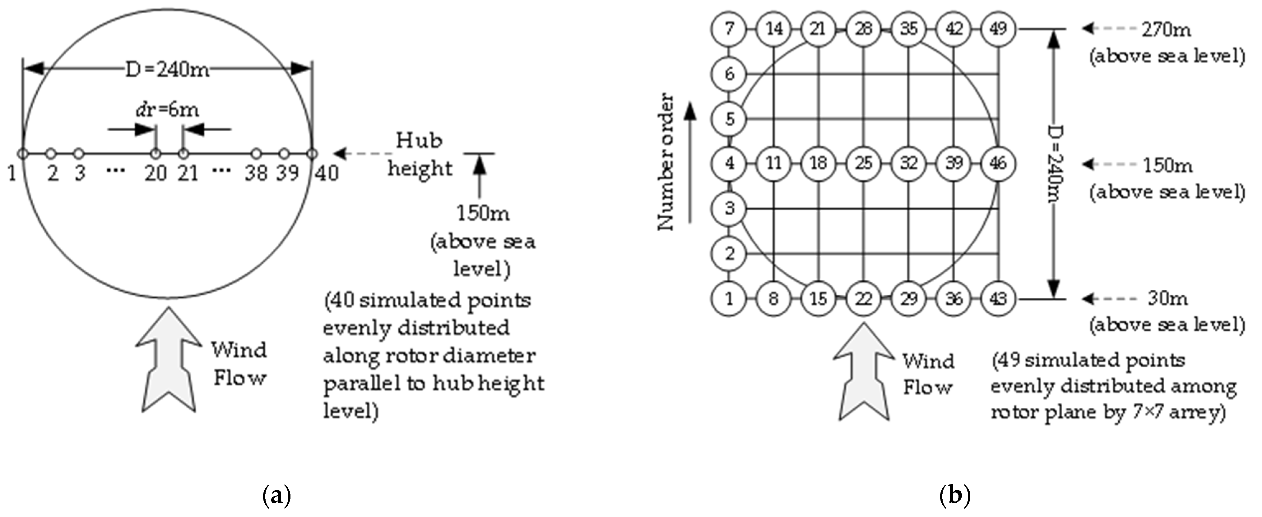
Set the basic parameters of the simulated wind field, including simulation points $\mathrm{m}$, simulation height $z$, and spacing between simulation points $\mathrm{dr}$, etc.

$$dr=\left(\frac{z}{m-1}\right)\cdot \sqrt{{\left(x_k-x_j\right)}^2+{(y_k-y_j)}^2}$$

(3)

where, $x_k,x_j,y_k,y_j$ represent the abscissa and ordinate values of simulation point $k$ and simulation point $j$, respectively.

(4)

Calculate the cross-spectral density matrix of each frequency sampling point $\left\{S\left(f_n\right)\right\}$, $(n=1,2,3,\cdots ,N)$:

$$S\left(f_n\right)=\left[\begin{array}{cccc}{S}_{11}& S_{12}& \cdots & S_{1m}\\ S_{21}& S_{22}& \cdots & S_{2m}\\ ⋮& ⋮& \ddots & ⋮\\ S_{m1}& S_{m2}& \cdots & S_{mm}\end{array}\right]$$

(4)

where, $S\left(f\right)$ denotes the power spectral density function, $S_{jj}$ denotes the autocorrelation spectrum of corresponding points, and $S_{kj}\left(k\ne j\right)$ denotes the cross-correlation spectrum between two simulated points, $(k=1,2,3,\cdots ,j)$, which can be calculated as:

$$S_{kj}(f_n)=\sqrt{S_k\left(f_n\right)S_j\left(f_n\right)}\cdot coh\left(k,j;f\right)$$

(5)

Since the cross-correlation function of the fluctuating wind speed in one-dimensional space does not involve the change of height, the cross-correlation spectrum between the simulated point $\mathrm{j}$ and other simulated points is consistent, and the cross-correlation spectrum of the fluctuating wind speed in one-dimensional space can be obtained by the following formula:

$$S_{kj}(f_n)=S_j\left(f_n\right)\cdot coh\left(k,j;f\right)$$

(6)

(5)

Combined with the double-indexed frequency method, the Cholesky decomposition method is performed on the cross-spectral density matrix of sampling points at each frequency, and the decomposed lower triangular matrix is obtained, that is:

$$S\left(f_{kn}\right)=H\left(f_{kn}\right)H^T\left(f_{kn}\right)$$

(7)

$$f_{kn}=\left(n-1\right)df+\left(k/m\right)df$$

(8)

where, $f_{kn}$ denotes the double-indexed frequency; $H(f_{kn})$ denotes the decomposed lower triangular matrix.

(6)

Random phase obedience ${\varphi }_{kn}$ is introduced and subjected to independent random distribution among intervals $\left(0,2\pi \right)$, carrying out the Fast Fourier transformation, namely:

$$G_{kn}(t)=FFT\left(B_{kn}\right)$$

(9)

$$B_{kn}\left(ndf\right)=\{\begin{array}{c}H\left(ndf+\left(k/m\right)df\right)e^{i{\varphi }_{kn}},(0\le n<N)\\ 0,(N\le n<M)\end{array}$$

(10)

(7)

Employing harmonic superposition method to generate the wind speed time history of the simulated point $j$ samples, and $v_j(t)$ can be calculated by Equation (11):

$$v_j\left(p\cdot dt\right)=\sqrt{2df}Re({\displaystyle \sum }_{k=1}^j{G}_{jk}exp(i\frac{k}{m}\cdot 2\pi df\cdot p\cdot dt)$$

(11)

where, $p=1,2,3,\cdots ,\left(M\cdot m-1\right)$.

2.3. Power Spectrum Correction Method

In the practical application of simulating a uniform pulsating wind field, since the dimensionless power density spectrum of one-dimensional space accords with Gaussian distribution (Figure 1 shows the longitudinal dimensionless wind speed power density spectrum curve of several classical spectra), the relationship between the simulating pulsating wind speed variances ${\sigma }^2$ and the power spectrum density function $S\left(f\right)$ is defined as below [18,19]:

$${\sigma }^2={{\displaystyle \int }}_0^{\infty }S\left(f\right)df$$

(12)

Therefore, when the analog frequency range $[F_{\max , }{F}_{min}]$ is a segment interval and is cut out from the spectral density function originally defined interval $\left(0,\infty \right)$, theoretically, the variance of the simulated fluctuating wind speed ${\sigma }_{theory}{}^2$ is defined as:

$${\sigma }_{theory}{}^2={{\displaystyle \int }}_{F_{min}}^{F_{max}}S\left(f\right)df$$

(13)

The defined standard deviation of the fluctuating wind speed $\sigma$ can be determined by an empirical formula in the simulation algorithm (e.g., Equation (20) in Section 3.1), according to the calculation formula of turbulence intensity $I_T=\sigma /v(t)$, choosing the segment interval $[F_{\max , }{F}_{min}]$ will cause the simulated results to produce truncated standard deviation, which will inevitably affect the numerical error of the simulated turbulence intensity due to the existence of the deviation of $\sigma$ and ${\sigma }_{theory}$. The deviation between the two can be calculated as:

$$\epsilon =\left|\frac{{\sigma }_{theory}-\sigma }{\sigma }\right|$$

(14)

The standard deviation’s deviation $\epsilon$ affects the simulated turbulence intensity to a certain extent, and the smaller the deviation is, the smaller the influence is.

It can be seen from Equations (12)–(14) that when increasing the proportion of the interval length in the simulated frequency interval, the theoretically calculated standard deviation’s deviation will decrease. However, it can be seen from the simulation algorithm introduced in Section 2.2 that the frequency step has a significant impact on the simulation results. On the other hand, according to the formula $df=\frac{F_{max}-F_{min}}{N}$, after determining the basic range of the simulation frequency interval, a slight change caused by the minor increase in cutoff frequency relative to the magnitude of $N$ is almost negligible. When the ratio of the turbulence integral length to the average wind speed $X_k=L_k/\overline{U}$ is constant, the upper limit of the interval expands to the right indefinitely, and the deviation will not significantly decrease [10].

This is also consistent with the simulation conclusion in this paper: under the same simulation conditions, when the initial frequency changes by one step unit, the impact on the standard deviation’s deviation $\epsilon$ is significantly greater than that when the cutoff frequency changes by one step unit (see Section 3.2 for details). In addition, the simulation results also show that the theoretical truncation bias $\epsilon$ caused by the truncation of the simulation frequency range will affect the numerical value of the simulated object in the simulation process, which leads to the simulation bias $\widehat{\epsilon }$. Simulation deviation is not only related to truncation deviation, but also to the setting of other simulation parameters and the application of interpolation methods. The simulated deviation is a manifestation of the error generated by simulating the turbulence intensity, which can be expressed by the following calculation formula:

$$\widehat{\epsilon }=\left|\frac{\widehat{\sigma }-\sigma }{\sigma }\right|$$

(15)

where, $\widehat{\sigma }$ denotes the standard deviation of actual simulated wind speed.

Considering $\mathrm{df}=\frac{F_{max}-F_{min}}{N}$, if the magnitude of the frequency sample $N$ is increased by an order (usually $N$ is an exponential form with base 2), the simulation bias can indeed be reduced, but at the same time the computational memory will be doubled and the simulation speed will be seriously slowed down. Take the analog frequency range $[F_{\max , }{F}_{min}]=[{10}^{-5},12]$, and the other simulation conditions are consistent with the case of one-dimensional simulation in Section 3. The simulation experiment results are shown in

Table 1. The relationship between the frequency sampling points scale and simulated deviation.

Test No.	Test 1	Test 2	Test 3
magnitude of $N$	$N=2^{12}$	$N=2^{13}$	$N=2^{14}$
${\widehat{\epsilon }}_{min}$	0.0026	0.0026	0.0131
${\widehat{\epsilon }}_{ave}$	0.2146	0.1151	0.0615
${\widehat{\epsilon }}_{max}$	0.3998	0.2122	0.1049
CPU time	40s	84s	212s

.

Table 1 and Figure 2 show that increasing the scale $N$ causes the whole standard deviation bias of the turbulent wind field simulation to almost linearly reduce, or even when increased to $N=2^{14}$, the overall standard deviation’s bias of the turbulent wind field has reached the truncation error, but with a significant disadvantage of longer running time, and a great computing cost if more simulated points are set in the turbulent wind field space. On the other hand, this result is not very ideal. When increasing the magnitude of $N$, the simulated turbulence intensity of more simulation points falls outside the range of reference turbulence intensity and the defined turbulence intensity and needs to be removed, resulting in an unnecessary waste of computing resources.

To sum up, the correction method should realize the minimum truncation deviation ${\epsilon }_{min}$ in theory and the minimum simulation deviation ${\widehat{\epsilon }}_{min}$ generated in the actual simulation process, without adding more frequency sampling points to reduce the simulation efficiency. In addition, the method should generate as many effective simulation points as possible (effective simulation points are defined as the simulation points whose simulated turbulence intensity ${\widehat{I}}_T$ falls within the range of reference turbulence intensity $I_{ref}$ and defined turbulence intensity $I_T$).

Consider the error values of truncation bias $\epsilon$ and simulation bias $\widehat{\epsilon }$:

$$\mathsf{\Delta }\epsilon =\widehat{\epsilon }-\epsilon$$

(16)

Introduce compensation coefficient $\beta$:

$$\beta ={(1+\mathsf{\Delta }\epsilon )}^2$$

(17)

If the variance ${\sigma }^2$ in the PSD function is substituted into the compensation coefficient $\beta$, then the original factor will be corrected $\frac{{\sigma }^2}{\beta }$.

3. Results and Discussion

Given the IEA 15 MW (NREL) wind turbine [20], its basic parameters are shown in

Table 2. 15 WM wind turbine parameters.

capacity	15 MW
wind turbine diameter $D$	240 m
hub height $Z$	150 m
the reference mean wind speed $V_{ref}$	10.59 m/s
reference turbulence intensity $I_{ref}$	0.14

, and frequency domain simulation parameter settings as shown in

Table 3. Frequency domain simulation parameters.

	One-Dimensional Space	Two-Dimensional Space
number of simulated points $m$	40	49
simulated point spacing $dr$	$6\left(k-j\right)$	Calculate according to the Formula (3) in Section 2.2
frequency sampling number $N$	$2^{12}$	$2^{12}$
analog time points $M$	$2^{13}$	$2^{13}$

.

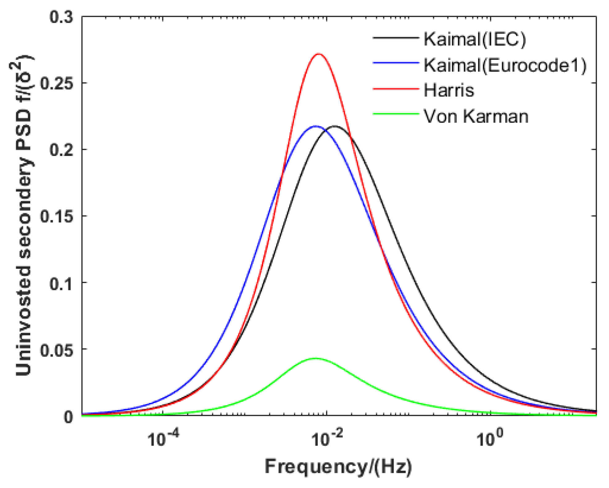
3.1. Power Density Spectrum and Coherence Function Selection

Kaimal spectrum is widely used to describe the spectral density during wind speed [21], and its simulation results are more conservative when applied to the fatigue load design of wind turbines. The function expression of Kaimal spectrum in IEC61400-1 4th Edition [18] is as below, $X_k=L_k/\overline{U}$ represents the ratio of the turbulence integral length to average wind speed ($k=1,2,3$ represents the longitudinal, transverse and vertical component spectra, respectively):

$$S\left(f\right)={\sigma }_k{}^2\frac{4X_k}{{(1+6f{X}_k)}^{5/3}}$$

(18)

IEC61400-1 uses an exponential form of coherence function, which is expressed as follows:

$$Coh\left(r,f\right)=exp[-12({(\frac{fr}{u})}^2+\left(0.12\frac{r}{L_k}{)}^2{)}^{0.5}\right]$$

(19)

In Equation (18), according to IEC61400-1, the parameters of the longitudinal component are calculated as follows:

(1)

Wind speed definition standard deviation ${\sigma }_1$:

$${\sigma }_1=I_{ref}\left(0.75\overline{U}+b\right); b=5.6m/s$$

(20)

where, $I_{ref}=0.14$, determined by 15 MW wind turbine design grade Class IB; $\overline{U}=10.59 m/s$.

(2)

Integral scale parameter $L_1$:

$$L_1=8.1{\Lambda }_1$$

(21)

The longitudinal integral scale parameters at the height of the hub $Z$ are:

$${\Lambda }_1=\{\begin{array}{c}0.7Z,\left(Z\le 60 m\right)\\ 42 m,\left(Z\ge 60 m\right)\end{array}$$

(22)

The horizontal and vertical components of turbulence spectrum parameters simulating a three-dimensional fluctuating wind speed are shown in

Table 4. Turbulence spectrum parameters of horizontal and vertical components.

Main Parameters	${\mathit{\sigma }}_{\mathit{k}}$	${\mathit{L}}_{\mathit{k}}$
the transverse (k = 2)	$0.8{\sigma }_1$	$2.7{\Lambda }_1$
the vertical (k = 3)	$0.5{\sigma }_1$	$0.66{\Lambda }_1$

.

3.2. Determine the Analog Frequency Range $[F_{max,}{F}_{min}]$

By setting the initial frequency $F_{min}\in \left[{10}^{-5},{10}^{-1}\right]$, setting the cut-off frequency $F_{max}\in \left[1,10\right]$ (step by ${10}^1$ units and $1$ unit respectively to form an $5\times 10$ analog frequency interval matrix), and performing integral operations one by one according to Equation (13), the ratio of the standard deviation of the truncated interval integral to the standard deviation of the fully defined interval integral is $\eta ={\sigma }_{theory}/\sigma$, the result of which is shown in Figure 3a. By combining this with the $3\sigma$ principle, it can be found that when the initial frequency $F_{min}<{10}^{-4}$ and cut-off frequency is given any value, the standard deviation ratio $\eta$ will always fall within a confidence interval of $+2\sigma$, as the cutoff frequency increases, $\eta$ infinity goes to $+3\sigma$, therefore, it achieves a value of $F_{min}={10}^{-4}$.

Under the same simulation conditions, the simulation frequency interval element from the matrix described above was substituted, one by one, into the uniform turbulent wind field simulation algorithm, for simulating fluctuating wind speed of time history in one-dimensional space (at hub height), accompanied with the standard deviation’s deviation and truncation deviation. The comparison between the two is shown in Figure 4b. The figure shows that when $F_{min}={10}^{-4}$, the simulation bias $\widehat{\epsilon }$ does not decrease significantly with the increase of the simulation frequency range, the truncated bias step rises when $F_{max}>6$, instead. To weaken the distortion of the analog signal, the cutoff frequency $F_{max}=5$ was selected to simulate the uniform turbulent wind field in one-dimensional space (at the height of the hub) and two-dimensional space (at the swept surface of the wind wheel), respectively, (the distribution of simulated points of these two types of spatial wind field simulation are shown in Figure 4a,b, as above) considering the truncation error and simulation error comprehensively, and the compensation coefficient was determined.

3.3. Compensation Coefficient $\beta$ Correction Method

According to Section 3.2, the time history simulation of the fluctuating wind speed in a turbulent wind field is performed under the condition that the simulated frequency range is determined as $[F_{\max , }{F}_{min}]=[{10}^{-4},5]$. The main parameters are shown in

Table 5. The compensation coefficient of relevant parameters.

Object Parameters	Numerical Value
fully defined standard deviation $\sigma$	2.2727
truncated standard deviation ${\sigma }_{theory}$	2.2476
the standard deviation of wind field simulation $\widehat{\sigma }$	2.4883
truncated standard deviation’s bias $\epsilon$	0.0110
simulated standard deviation’s bias $\widehat{\epsilon }$	0.0949

, and the distribution of the standard deviation error and compensation coefficient at each simulated height in space is obtained, as shown in the Figure 5.

The longitudinal Kaimal spectrum is modified by considering the compensation coefficient $\beta$:

$$S^0\left(f\right)=\frac{{\sigma }_1{}^2}{\beta }\frac{4X_1}{{(1+6f{X}_1)}^{5/3}}$$

(23)

where, $X_1=L_1/\overline{U}$.

After compensation and correction, the main parameters of one-dimensional space are shown in

Table 6. Parameters’ contrast between being corrected and uncorrected.

Mock Generated Objects		Uncorrected	Corrected
simulated standard deviation $\hat{\mathsf{\sigma }}$	Maximum	2.7103	2.4802
	Minimum	2.1604	1.9818
	Average	2.4883	2.2954
simulated standard deviation’s bias $\hat{\mathsf{\epsilon }}$	Maximum	0.1925	0.1280
	Minimum	0.0024	0.0031
	Average	0.1020	0.01
simulated turbulence intensity ${\widehat{\mathrm{I}}}_{\mathrm{T}}$		0.1755	0.1619

.

The modified simulated point fluctuating wind speed diagram is shown as Figure 6.

A comparison of the power spectral density at simulated points and power spectral density related to simulated wind speed before and after modification is shown in Figure 7. Among which, the line of the ‘Corrected Spectrum Simulated’ represents the power density spectrum of the fluctuating wind speeds that are generated by the corrected Kaimal spectrum; the line of the ‘Corrected Spectrum’ represents the corrected Kaimal power density spectrum itself; the line of the ‘Original Simulated Spectrum’ represents the power density spectrum of the fluctuating wind speed that are generated by the original Kaimal spectrum; the line of the ‘Original Spectrum’ represents the original Kaimal power density spectrum itself.

Comparison of the standard deviation, standard deviation’s bias, and turbulence intensity of the simulated wind speed before and after modification is shown in Figure 8. Among which, in Figure 8a,c,e, the line of the ‘Corrected Simulation’ represents the standard deviation/standard deviation’s deviation/turbulence intensity of the fluctuating wind speed that is simulated by corrected Kaimal spectrum and generated by 40 points in a one-dimensional simulated wind field; the line of the ‘Original Simulation’ represents the standard deviation/standard deviation’s deviation/turbulence intensity of the fluctuating wind speed that is simulated by the Kaimal spectrum and generated by 40 points in a one-dimensional simulated wind field; the line of the ‘Corrected mean value’ represents the mean value of the simulation results from the corrected Kaimal spectrum among 40 points in a one-dimensional simulated wind field; the line of the ‘Original mean value’ represents the mean value of the simulation results from the Kaimal spectrum among 40 points in a one-dimensional simulated wind field; in Figure 8e, the line named ‘Defined’ represents the defined turbulence intensity $I_T$; the line named ‘Referenced’ represents the reference turbulence intensity $I_{ref}$; in Figure 8b,d,f, the surface named ‘Corrected’ represents the standard deviation/standard deviation’s deviation/turbulence intensity of the fluctuating wind speed of the points varying along with the simulated heights generated by the corrected Kaimal spectrum in a two-dimensional wind field; the surface named ‘Uncorrected’ represents the standard deviation/standard deviation’s deviation/turbulence intensity of the fluctuating wind speed of the points varying along with the simulated heights generated by the Kaimal spectrum in a two-dimensional wind field; and the surface named ‘Defined’ represents the defined standard deviation/turbulence intensity of the fluctuating wind speed of the points varying along the simulated heights.

Concerning the longitudinal one-dimensional space spectrum correction method and the lateral spectrum and the vertical spectrum parameters in Table 4, 20 evenly distributed simulation points are set to verify whether the compensate correction method suggested is applicable for the lateral spectrum and the vertical spectrum. A one-dimensional simulation of three-dimensional wind speed is acquired, and the three-dimensional fluctuating wind velocity contour map and 3 d surface figure of simulation point 10 are shown in Figure 9.

The above results show that:

(1)

The standard deviation $\widehat{\epsilon }$ generated by the Kaimal spectrum simulation of a one-dimensional turbulent wind field decreases from 0.102 to 0.01, and the reduction is 9.2 times, and the error of truncation deviation $\epsilon$ is only 10%;

(2)

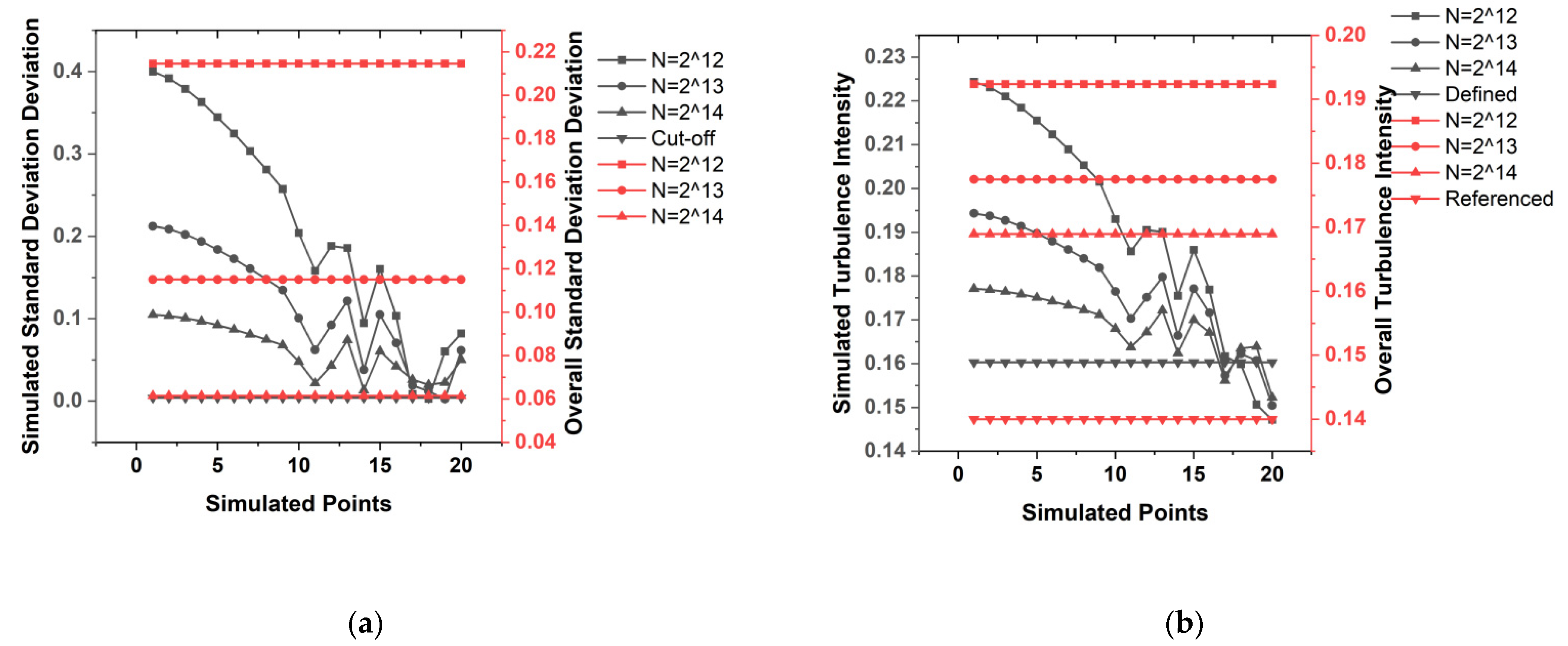
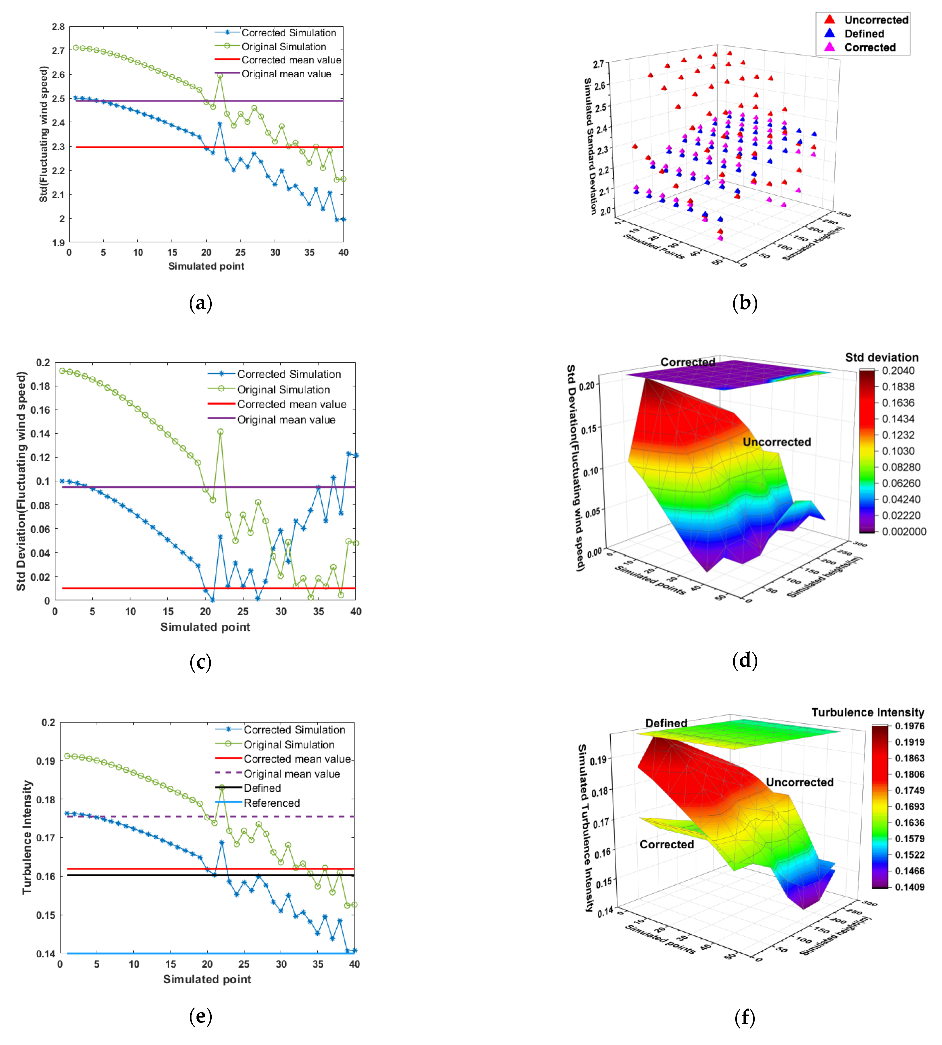
The numerical values of the Kaimal power density spectrum with a modified compensation coefficient $\beta$ simulating the overall turbulence intensity ${\widehat{I}}_T$ of the spatial turbulent wind field are closer to the defined turbulence intensity $I_T$, which is defined as the ratio of the fully defined standard deviation to the average wind speed $I_T=\sigma /\overline{U}$. In the one-dimensional wind field, the corrected Kaimal spectrum can provide more simulated points that are conservative, according to Figure 8a,c, and the mean value of standard deviation has declined by 0.2 point while the standard deviation’s deviation has dropped over 84.2%. Moreover, it can be drawn from Figure 8e that the turbulence intensity value of 45% (18/40) of the simulated points set in the simulation process finally reach the interval of [Referenced, Defined] after the spectrum is corrected, compared with that of the uncorrected spectrum simulation result, which has increased 35%. Therefore, the rate of efficient simulation points in the wind field has obtained a significant promotion. As can be seen from Figure 8e,f, the overall turbulence intensity of the compensated corrected turbulent wind field (referring to the “corrected mean value” line and “Defined” surface, respectively, in Figure 8) is very close to the turbulence intensity defined by the wind field;

(3)

The Kaimal power density spectrum simulation with the modified compensation coefficient $\beta$ generates a more simulated point of fluctuating wind speed turbulence intensity that is distributed within the IEC reference turbulence intensity and defined turbulence intensity range, which can be effectively used in load design evaluation;

(4)

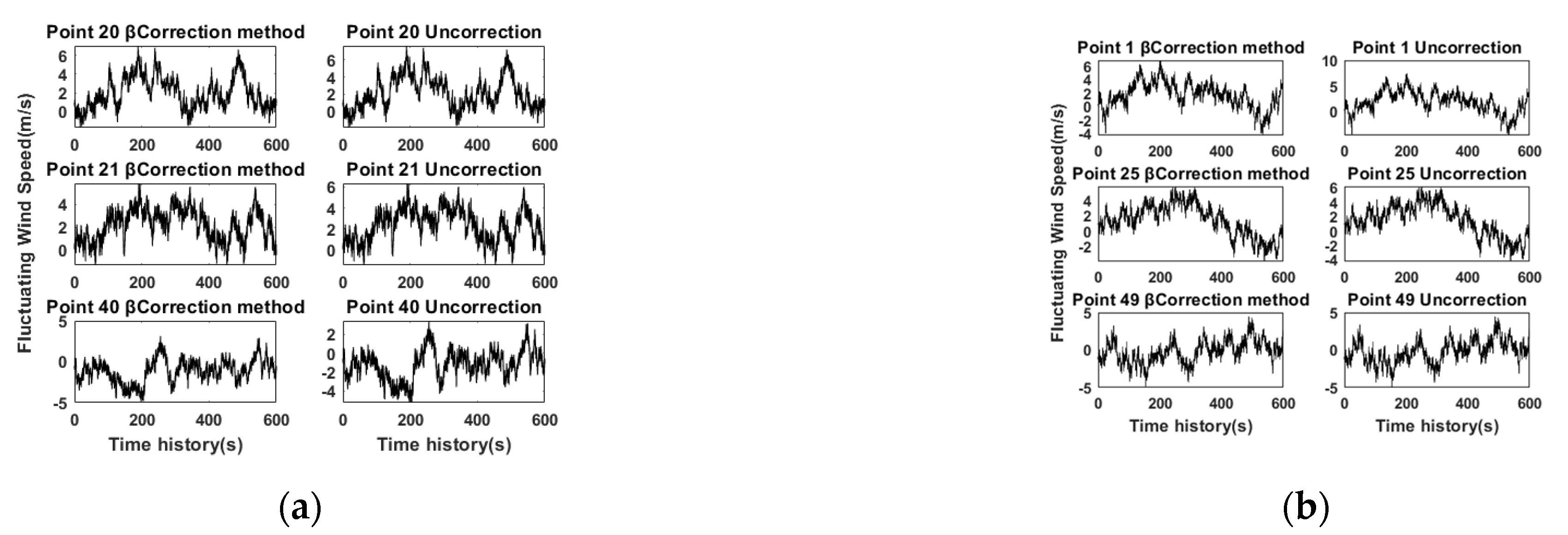
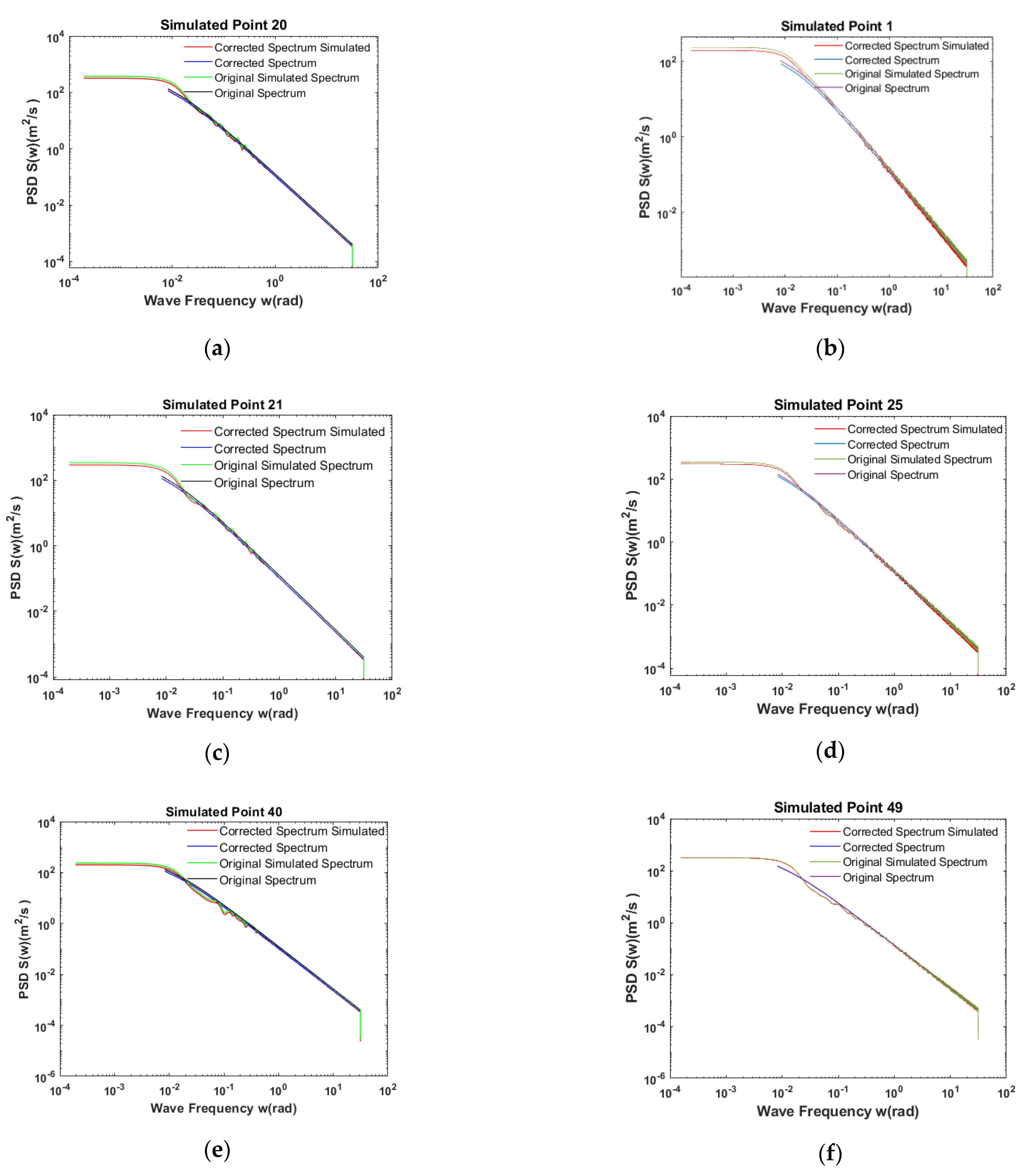
According to Figure 7, the line of the ‘Corrected Spectrum Simulated’ can always fit well with the line of the ‘Corrected Spectrum’, just like the line of the ‘Original Simulated Spectrum’ and the line of the ‘Original Spectrum’ does, which indicates that the fluctuating wind speed generated by the Kaimal power density spectrum simulation with the modified compensation coefficient $\beta$ can perfectly fit the modified self-power spectrum and meet the requirements of engineering applications.

4. Conclusions

(1)

The truncation standard deviation’s bias $\epsilon$ that is generated due to the simulated frequency range truncating from the fully defined range affects the simulated turbulent intensity ${\widehat{I}}_T$ of the fluctuating wind speed. Reducing the error between the truncation standard deviation ${\sigma }_{theory}$ and the defined standard deviation $\sigma$ can effectively reduce the effect and take the simulated turbulence intensity ${\widehat{I}}_T$ closer to the defined turbulence intensity $I_T$;

(2)

Under the same simulation conditions, the influence of the initial frequency $F_{min}$ on the truncation standard deviation’s bias $\epsilon$ is significantly greater than that of the cutoff frequency $F_{max}$. When $F_{min}<{10}^{-4}$, the ratio of truncation standard deviation ${\sigma }_{theory}$ to defined standard deviation $\sigma$ has fallen within the confidence interval of $2\sigma$. Under this value, the value range of cutoff frequency $F_{max}$ can be within [5,10], and the truncation deviation is small enough;

(3)

The turbulence intensity of the turbulent wind field simulated by the Kaimal spectrum of IEC61400-1 and IEC referenced the exponential coherent function is more conservative and more consistent with the defined turbulence intensity;

(4)

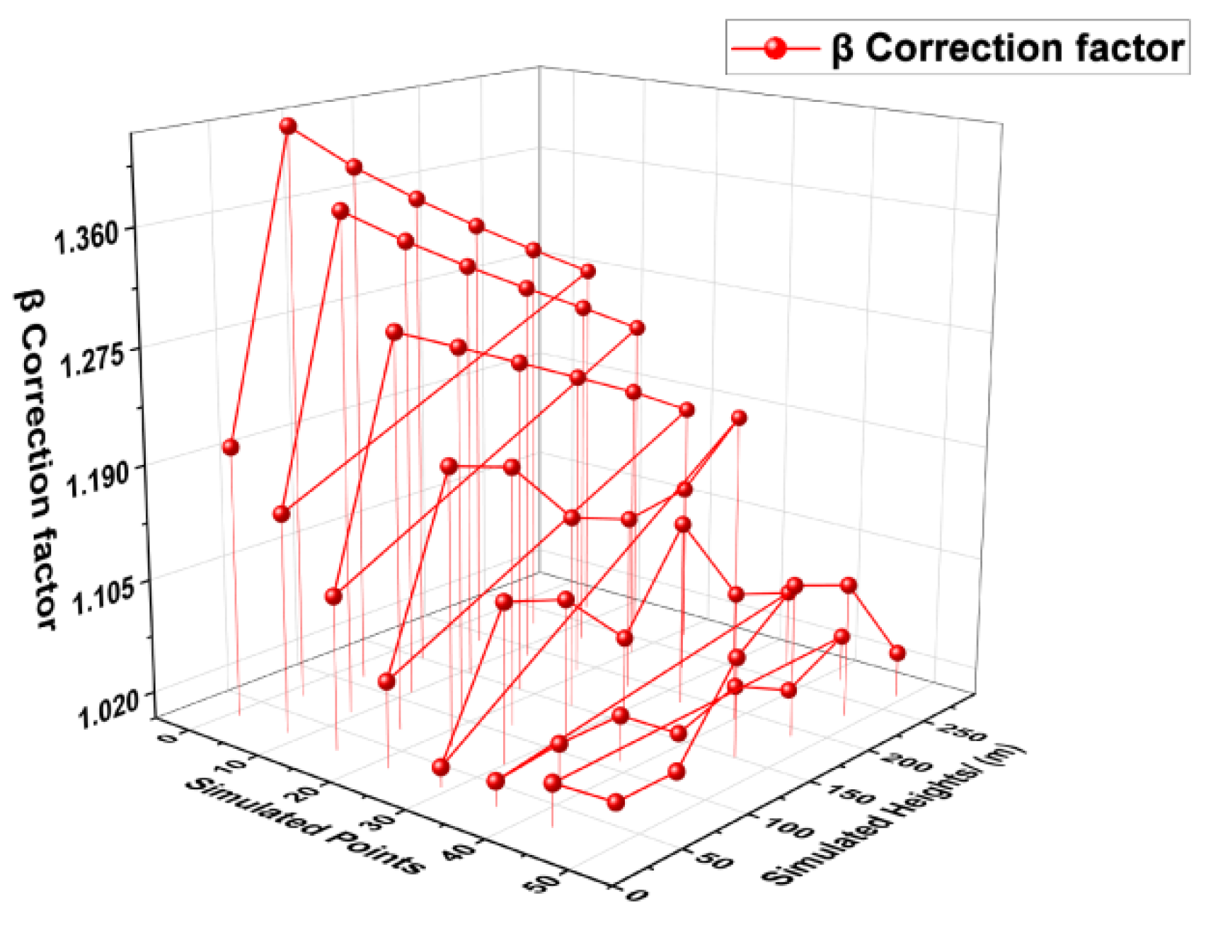
The calculation method of the compensation coefficient $\beta$ proposed in this paper is not that precise, for its value would change with the simulated height and distance. Nevertheless, the correction methodology can be employed to any wind speed PSD model for wind speed time-history simulation in uniform space.

References

- Bustamante, A.; Vera-Tudela, L.; Kuhn, M. Evaluation of wind farm effects on fatigue loads of an individual wind turbine at the EnBW Baltic 1 offshore wind farm. In Proceedings of the Wake Conference 2015, Visby, Sweden, 9–11 June 2015. [Google Scholar] [CrossRef] [Green Version]
- Chen, Y.; Zhang, J.; Wang, N. Wind turbine wind field models study numerical simulation of turbulence wind field with MATLAB. Acta Energiae Solaris Sinica 2006, 27, 954–960. [Google Scholar]
- Von Karman, T. Progress in the statistical theory of turbulence. Proc. Natl. Acad. Sci. USA 1948, 34, 530–539. [Google Scholar] [CrossRef] [PubMed] [Green Version]
- Harris, R.I. The nature of wind. In The Modern Design of Wind-Sensitive Structures; Construction Industry Research and Information Association: London, UK, 1971. [Google Scholar]
- Simiu, E. Wind spectrum dynamic along wind response. J. Struct. Div. 1974, 100, 203–209. [Google Scholar] [CrossRef]
- Kaimal, J.C.; Wyngaard, J.C.; Izumi, Y.; Coté, O.R. Spectral characteristics of surface-layer turbulence. Q. J. R. Meteorol. Soc. 1972, 98, 563–589. [Google Scholar] [CrossRef]
- Liang, J.; Chaudhuri, S.; Shinozuka, M. Simulation of nonstationary stochastic processes by spectral representation. J. Eng. Mech. 2007, 133, 616–627. [Google Scholar] [CrossRef]
- Shinozuka, M. Simulation of multivariate and multidimensional random process. J. Acoust. Soc. Am. 1971, 49, 357–368. [Google Scholar] [CrossRef]
- Ding, Q.; Zhu, L.; Xiang, H. An efficient ergodic simulation of multivariate stochastic process with spectral representation. Probabilistic Eng. Mech. 2011, 26, 350–356. [Google Scholar] [CrossRef]
- Tao, T.; Wang, H. Reduced simulation of the wind field based on Hermite interpolation. Eng. Mech. 2017, 34, 182–188. [Google Scholar] [CrossRef]
- Peng, L.; Huang, G.; Kareem, A.; Li, Y. An efficient space-time based simulation approach of wind velocity field with embedded conditional interpolation for unevenly spaced locations. Probabilistic Eng. Mech. 2016, 43, 156–168. [Google Scholar] [CrossRef] [Green Version]
- Chen, X.; Chen, J.; Li, J. Numerical simulation of fluctuating wind velocity time series of offshore wind turbine. Proc. CSEE 2008, 28, 111–116. [Google Scholar]
- Shen, G.H.; Huang, Q.Q.; Guo, Y.; Xing, Y.L.; Lou, W.J.; Sun, B.N. Simulation methods of fluctuating wind field and its application in wind-induced response of transmission lines. Acta Aerodyn. Sinica 2013, 31, 69–74. [Google Scholar] [CrossRef]
- Zhang, W.; Ma, C.; Sun, X.; Ju, X.L.; Liu, Y.C. Simulation of wind field with spacial correlation based on wavelet analysis method. Acta Aerodyn. Sinica 2008, 26, 425–429. [Google Scholar]
- Det Norske Veritas, Risø DTU National Laboratory. Guidelines for Design of Wind Turbines, 2nd ed.; China Machine Press: Beijing, China, 2011. [Google Scholar]
- Proakis, J.G.; Manolakis, D.G. Digital Signal Processing: Principle, Algorithms, and Applications; Electronic Industry Press: Beijing, China, 2014. [Google Scholar]
- Zhao, W.; Liao, M. A method for improving Kaimal spectrum and its algorithm implementation. Mech. Sci. Technol. Aerosp. Eng. 2013, 32, 1446–1450. [Google Scholar]
- IEC 61400-1. Wind Energy Generation Systems—Part 1: Design Requirements, 4th ed.; International Electrotechnical Commission: Geneva, Switzerland, 2019. [Google Scholar]
- Davenport, A.G. The spectrum of horizontal gustiness near the ground in high winds. Q. J. R. Meteorol. Soc. 1961, 87, 194–211. [Google Scholar] [CrossRef]
- IEA Task 37 2020 IEA GitHub Repository. Available online: https://github.com/IEAWindTask37/IEA-15-240-RWT (accessed on 11 August 2021).
- Hong, X.; Li, J. Stochastic Fourier Spectrum model and probabilistic information analysis for wind speed process. J. Wind Eng. Ind. Aerodyn. 2018, 1, 174. [Google Scholar] [CrossRef]