3D Stress Analysis of Multilayered Functionally Graded Plates and Shells under Moisture Conditions

Abstract

This paper presents the steady-state stress analysis of single-layered and multilayered plates and shells embedding Functionally Graded Material (FGM) layers under moisture conditions. This solution relies on an exact layer-wise approach; the formulation is unique despite the geometry. It studies spherical and cylindrical shells, cylinders, and plates in an orthogonal mixed curvilinear coordinate system ($\alpha$, $\beta$, z). The moisture conditions are defined at the external surfaces and evaluated in the thickness direction under steady-state conditions following three procedures. This solution handles the 3D Fick diffusion equation, the 1D Fick diffusion equation, and the a priori assumed linear profile. The paper discusses their assumptions and the different results they deliver. Once defined, the moisture content acts as an external load; this leads to a system of three non-homogeneous second-order differential equilibrium equations. The 3D problem is reduced to a system of partial differential equations in the thickness coordinate, solved via the exponential matrix method. It returns the displacements and their z-derivatives as a direct result. The paper validates the model by comparing the results with 3D analytical models proposed in the literature and numerical models. Then, new results are presented for one-layered and multilayered FGM plates, cylinders, and cylindrical and spherical shells, considering different moisture contents, thickness ratios, and material laws.

1. Introduction

The environmental conditions characterizing the service life of structural components can be adverse in many applications. The aerospace field gives several examples of changing environments, which results in temperature gradients and moisture concentration variability. It is crucial to consider such two factors and to include them in a proper structural analysis: the thermal and hygrometric fields induce an internal stress distribution, which changes as soon as the environmental conditions change. As with any stress field, it might induce failures on the structure [1], either on its own or because it sums up to that caused by classical mechanical loads. Composite, multilayered, and FGM-embedding structures require a special focus. Composite materials can also be degraded by moisture absorption and the following diffusion through the matrix [2]; multilayered structures highlight a strong heterogeneity in the hygro/thermal/mechanical properties; FGMs induce a further complication due to non-constant terms in governing equations. However, their boosted implementation in critical structural applications recently increased the attention of the researchers on these effects.

Laminated structures and composite materials suffer from a clear variation of the properties at the interfaces, which is the critical source of the delamination process [3]. Eliminating this discontinuity and substituting it with a smooth trend is the key achievement of Functionally Graded Materials (FGMs). They are advanced composite materials made by two or more different phases mixed with a continuous graded distribution. As a result, they are heterogeneous materials, delivering optimized responses for each application: the advancements in processing technologies made it possible to control a unidirectional and even multidirectional variation. Combinations of a metallic and a ceramic phase are classic examples of FGMs finding application in severe thermal environments: they overcome the differences in thermal properties of the two constituents and, at the same time, deliver a reduced thermal stress distribution. Stiffness coefficients, hardness, thermal conductivity, moisture diffusivity, and corrosion resistance are just some examples of the performance characteristics that can be combined and enhanced [4].

Several recent and relevant works focused on structures embedding FG layers underline their importance in practical applications. From an analytical perspective, Sobhani et al. recently proposed several analytical results in the frame of the vibration analysis of FG shells. First, the governing equations followed the First-order Shear Deformation Theory (FSDT); then, they used the Generalized Differential Quadrature Method (GDQM), a semi-analytical solution method, to solve the system of partial differential equations. They studied conical shells embedding hybrid matrix/fiber nanocomposites in [5]; the approach was then extended to paraboloidal and hyperboloidal shells embedding polymer matrix, carbon fiber, and graphene nanoplatelets in [6]. Using the same approach, they studied sandwich conical-cylindrical-conical shells [7]. The layers are reinforced with functionally graded carbon nanotubes and graphene nanoplatelets; they described the elastic coefficients following an Equivalent Single Layer approach. They also studied five different patterns of CNT fibers distribution inside of the matrix while defining the vibrational behavior of coupled conical-conical shells [8]. They used the five-parameter shell theory and solved the differential equations through GDQM. Three-phase nanocomposites were also studied in hemispherical-cylindrical shells exploiting a similar approach [9] and defining the governing equations through the first-order shear deformation theory. From a numerical perspective, Rezaiee-Pajand et al. studied sandwich beams embedding FGM in two ways: they applied the Ritz method and the principle of minimum total potential energy within the framework of Timoshenko and Reddy beam theories in [10] to assess the bending of beams with different cross sections; they also developed a four-node isoparametric beam element to study porous beams with FGM [11]. Concerning two-dimensional geometries, the same authors proposed the nonlinear analysis of FG shells in [12,13] by improving an isoparametric six-node TRIA element with strain interpolation functions; the mechanical properties grading followed a power low. They also proposed a three-node TRIA element [14] using a mixed strain finite element approach and demonstrated that it is possible to get the exact response of the beams with a low number of elements under large deformations.

The solutions available in the literature seem to be promising. However, the results of a hygrometric stress analysis depend not only on the capabilities of the elastic model implemented but also on how the moisture content field has been evaluated, given the external boundary conditions. The hygrometric field acts as a field load; its quantification necessarily influences the stress analysis results. Aerospace applications usually involve thin components. Consequently, evaluating the moisture content field translates into determining its profile along with the thickness direction, generally coinciding with the grading direction of the mechanical/hygrometric properties. Developing a mechanical/elastic model for a thin component can be done at different levels of detail: 3D or 2D approaches, coupled with an analytical or numerical method. However, this might not be sufficient in defining the refinement of a model when hygrometric stresses are concerned. Even an analytical, exact 3D model would give wrong results when fed from an inaccurate moisture content field. The molecular diffusion depends on the gradient of the concentration and is described by Fick’s law. A solid mathematical analogy between Fick’s law and the Fourier heat conduction equation strongly simplifies the analysis and the dissertation. An exact solution comes from resolving three-dimensionally the diffusion/conduction equations; however, simplified solutions might benefit from their unidirectional simplification or an assumed-linear profile. Those three situations require an external evaluation of the moisture content field before the mechanical analysis. An alternative consists in defining a coupled hygro-mechanical model, in which the moisture content field is a primary variable of the problem in analogy with the thermal field [15,16,17,18,19,20].

This paper discusses an hygro-elastic shell model, which relies on the exponential matrix method. This model does not limit to a specific geometry or lamination scheme; on the contrary, it handles plates, cylindrical, and spherical shells. Furthermore, it accepts one or more FGM layers on their own or coupled with homogeneous layers (sandwiches give an example). It extends the authors’ 3D exact thermo-elastic shell model discussed in [21] to hygro-elastic stress analysis. The problem is defined under steady-state conditions only; the solution requires the moisture content amplitudes at the top and bottom external surfaces to be specified. As a first step, the solution evaluates the moisture content profile through the thickness direction. The authors considered three possible options: the 3D Fick diffusion law, its 1D simplified version, and an a priori assumed linear trend. Despite this, the model handles the solution via a layer-wise approach and through the exponential matrix method. The present authors are not the only ones using the exponential matrix method for solving the differential equilibrium equations. Soldatos and Ye [22] already used it in analyzing the free vibrations of cylinders; Messina [23] applied it to study multilayered plates. The orthogonal mixed curvilinear coordinate system helped study spherical shells in [24] using three transverse stress and three displacement components as primary variables of the problem. The analytical procedure is in analogy with the free vibration analysis and the static analysis under mechanical load discussed by the first author in [25,26,27,28,29,30]. Those previous formulations already handled different materials and geometries but lacked loads other than the mechanical ones. In those simpler cases, a set of three homogeneous differential equations are at the basis of the problem. However, the hygrometric load adds an additional term that makes them not homogeneous. The exponential matrix method also handles this feature, as discussed in [21] for the thermoelastic stress analysis of shells with FGMs. The closed-form solution of the problem is possible given the harmonic forms imposed on the variables (displacements and hygrometric field) and the simply supported boundary conditions. Moreover, the whole formulation benefits an orthogonal mixed curvilinear coordinate system, following the suggestions in [31,32,33,34]. This strategy introduces a set of curvature terms, the elements through which the equations automatically adapt to the different geometries. Such terms are a function of the thickness coordinate, together with the elastic and hygrometric coefficients in FGM layers. Introducing a set of fictitious (mathematical) layers allows obtaining constant coefficients and using the method discussed in [35] to solve the problem.

The literature overview offers different analytical and numerical 2D models handling the hygrometric stress analysis; they specifically focus on multilayered structures. Far fewer discuss the problem of structures embedding FGMs. The literature overview will demonstrate that, to the authors’ knowledge, no analytical 3D shell model exists, in which the structures are different, provided that they have constant radii of curvature, and the moisture content evaluation follows three different approaches. Laoufi [36] studied rectangular plates embedding FGMs when subjected to different boundary conditions, including moisture content and temperature field. They developed an analytical method through the hyperbolic shear deformation plate model, which satisfied the stress boundary conditions and required no shear corrections. The volume fractions of the ceramic-metal constituents were used to define the materials grading in the thickness direction following a power law. The same power law was included in Inala’s work [37], devoted to studying how the hygrothermal environment affects the vibration characteristics of plates embedding FGMs. To do this, the author developed a finite element model of the structures under investigation. Dai [38] and his colleagues focused on circular plates with a variable thickness along with the radial direction. They derived nonlinear governing equations for temperature, moisture content, and displacement fields and solved them through the differential quadrature method. Zenkour also studied how the thermal and hygrometric fields affect the bending and the buckling of plates embedding FGMs [39]. In this case, also, the authors considered a material grading in the thickness direction of the structure. Their formulation relies on an exponential shear deformation theory and applies to plates resting on elastic foundations. Hamilton’s principle was used to derive the equilibrium equations, and Navier’s method to obtain the results. Boukelf also studied plates resting on elastic foundations, embedding FGMs [40]. The author developed a novel higher-order shear deformation theory model, deducing the problem equations through the virtual work principle. Hygro, thermal, and mechanical loads are all properties that can be handled. Analogously, Zidi [41] developed a further model for the same issue. In this case, the author used a four-variable refined plate theory. Analogous research has been proposed in [42] concerning functionally graded beams. The author deepened the influence of moisture content field and temperature on the bost-buckling response of beams. A nonlinear finite element solution was considered, in which the authors handled the kinematics of the bost-buckling through the Lagrangian approach.

More substantial is the literature discussing the moisture content effects on isotropic, orthotropic, and laminated structures. Chiba and Sugano [43] studied multilayered plates and proposed a two-dimensional analytical solution for hygrothermal effects on multilayered plates. The Classical Lamination Plate Theory and an analytical 3D plate model were compared in [44,45] while performing the hygro-thermal stress analysis. The CLT also received the attention of Kalil [46] when he investigated composite plates. Kollar [47] made an analytical investigation of composite cylindrical shells, while Shen [48] focused on buckling and post-buckling behaviors. The CLT was found to be inadequate in hygrothermal mechanical analysis by Lee and his colleagues [49]. There is no shortage of numerical models in this field; an example is given in [50], where plates with a central hole were studied. Multilayered structures under hygrometric fields have been the target of the finite element model by Khoshbakht et al. [51]; Kundu and Han studied buckling and vibration in multilayered shells with double curvature [52] through a finite element model grasping the hygrothermal effects. They extended this research to dynamic instability of doubly-curved shells embedding composite materials through a nonlinear finite element under orthogonal curvilinear coordinates [53]. Marques and Creus included the Fick diffusion law [54] into a FE shell model devoted to isotropic and multilayered structures under a hygrothermal environment. With the same aim, Naidu and Sinha [55] investigated cylindrical shell panels under large deflections through a higher-order shear deformation theory. Patel also proposed a higher-order FE for laminated parts [56]. Sereir et al. [57,58,59] considered the elastic properties variation in composite plates with the temperature and the moisture content and discussed a transient hygroscopic stress analysis. In [60,61,62,63], simplified solutions for hygro-thermal stresses analysis of composite plates considering the variation in elastic properties due to the hygrothermal environment are also considered. An analogous evaluation devoted to dynamic behavior has been proposed in [64,65]. Ghosh [66] used a FE model to investigate how a severe hygrothermal environment can affect the initiation and progress of damages in composites.

The literature survey highlighted that the hygromechanical stress analysis of structures embedding FGM layers still misses general and exact solutions as benchmarks in new solutions. Instead, the only analytical models work on defined and specific boundary conditions, laminations, and geometry. This paper intends to fill this gap by extending the authors’ previous work on multilayered structures to FGMs. The manuscript is organized as follows. Section 3 describes the hygro-elastic shell problem and its solution with the exponential matrix method. Section 2 explores the moisture diffusion problem with the three approaches introduced before. The Fick law of diffusion has the same mathematical formulation of the Fourier heat conduction equation; the moisture diffusion problem and the heat conduction problem are in analogy, indeed, as demonstrated in [67], and further confirmed by Tay and Goh [68,69]. Therefore, Section 2 quantifies the moisture content profiles. Solving the 3D Fick diffusion law is possible by exploiting the analogy with the heat conduction problem. Tungikar and Rao [35] give a methodology that can also be applied in this context; the unidimensional Fick diffusion law disregards the diffusion fluxes in directions other than the thickness coordinate and can be calculated in analogy. Section 4 gives two sets of results. The first set, labeled as Assessments, is introduced to validate the problem. In the absence of 3D exact solutions for hygro-elastic problems in shells with FGM layers, the section exploits existing results for thermal stress analysis. After validating the present model and an additional FE model, the section uses this last FE model to verify the results when the hygrometric load replaces the thermal one. The second set, labeled as Benchmarks, discusses new results, which introduce further comments on the effects of moisture content profiles, thickness ratio, material, and lamination scheme, together with the impact of the geometry. The main conclusions and the further development are then summarized in Section 5.

2. Fick Moisture Diffusion Equation

This model relies on a decoupled solution, which means that the moisture content is evaluated separately and enters the elastic part of the problem as a known term. The essential hypothesis to obtain exact closed-form solutions is that all the problem variables have a harmonic form. For what concerns the moisture content, this means

$$\begin{array}{cc}\hfill {\mathcal{M}}^k(\alpha ,\beta ,z)& =M^k\left(z\right)sin\left(\overline{\alpha }\alpha \right)sin\left(\overline{\beta }\beta \right),\hfill \end{array}$$

(1)

$M^k\left(z\right)$ indicates the moisture content amplitude. Referring to Figure 1 and Figure 2: m and n are the half-wave numbers in the two in-plane directions $\alpha$ and $\beta$, respectively. a and b are the shell dimensions referred to the mid-surface ${\Omega }_0$; they allow calculating the terms $\overline{\alpha }=\frac{m\pi }{a}$ and $\overline{\beta }=\frac{n\pi }{b}$. Note that the harmonic form of the moisture content reduces its assessment to its profile along with the thickness direction z. What happens in $\alpha$ and $\beta$ directions is already defined through the sinusoidal functions.

The hygrometric boundary conditions are the moisture content amplitudes at the bottom and the top of the shell, $M_b$, and $M_t$, respectively. Three approaches exist to evaluate the moisture content profile; this solution implements all three, allowing a homogeneous comparison among them and with other methods. The solution is accomplished in analogy with what the authors achieved in [21] concerning the temperature field. Indeed, the Fourier heat conduction equation, regulating the thermal phenomenon, features the same mathematical expression of the Fick diffusion law, which applies to the moisture diffusion problem. The three approaches are here listed:

• the moisture content profile is defined by solving the 3D Fick diffusion law; the hygro-elastic model considering it takes the name of 3D(${\mathcal{M}}_c$,3D);
• the moisture content profile is defined by solving the 1D version of the Fick diffusion law; the hygro-elastic model considering it takes the name of 3D(${\mathcal{M}}_c$,1D);
• the moisture content profile is “a-priori” assumed as linear along with the thickness direction; the hygro-elastic model considering it takes the name of 3D(${\mathcal{M}}_a$).

All the acronyms report the term 3D: it states that the elastic part of the shell model relies on a three-dimensional solution. Instead, the part of the acronym inside the parentheses defines how the moisture content profile has been quantified. “c” means calculated, either via the 3D or the 1D Fick diffusion laws; “a” means linear assumed.

2.1. 3D Fick Equation

By analogy with the heat flux $\mathit{q}$, suppose to define a moisture flux $\mathit{g}$. Then, the differential equation of moisture diffusion into a homogeneous solid, in the absence of chemical reactions and under steady-state conditions ($\frac{\partial \mathcal{M}}{\partial t}=0$) reads:

$$\nabla ·\mathit{g}(u_1,u_2,u_3)=0.$$

(2)

Equation (2) is written in a general orthogonal curvilinear coordinate system $(u_1,u_2,u_3)$; however, in these conditions, the divergence of the moisture flux takes the following expression:

$$\nabla ·\mathit{g}=\frac{1}{a}\left[\frac{\partial }{\partial u_1}\left(\frac{a}{a_1}{g}_1\right)+\frac{\partial }{\partial u_2}\left(\frac{a}{a_2}{g}_2\right)+\frac{\partial }{\partial u_3}\left(\frac{a}{a_3}{g}_3\right)\right],$$

(3)

$g_1,g_2,g_3$ express the components of the 3D flux in directions 1, 2, and 3; their explicit form is

$$g_i=-{\mathcal{D}}_i\frac{1}{a_i}\frac{\partial \mathcal{M}}{\partial u_i},$$

(4)

${\mathcal{D}}_i$ is the diffusion coefficient along with direction i; $a_1$, $a_2$, and $a_3$ are the so-called scale factors, with a the product of the three factors ($a=a_1{a}_2{a}_3$). The problem takes place in a mixed curvilinear orthogonal coordinate system ($\alpha ,\beta ,z$); Povstenko [32] discussed that, in this context, Equation (3) might be rewritten as follows:

$$\frac{1}{H_{\alpha }{H}_{\beta }}\left[\frac{\partial }{\partial \alpha }\left(\frac{H_{\alpha }{H}_{\beta }}{H_{\alpha }}{\mathcal{D}}_1\frac{1}{H_{\alpha }}\frac{\partial \mathcal{M}}{\partial \alpha }\right)+\frac{\partial }{\partial \beta }\left(\frac{H_{\alpha }{H}_{\beta }}{H_{\beta }}{\mathcal{D}}_2\frac{1}{H_{\beta }}\frac{\partial \mathcal{M}}{\partial \beta }\right)\right]+{\mathcal{D}}_3\frac{{\partial }^2\mathcal{M}}{\partial z^2}=0,$$

(5)

FGM layers distinguish from classical isotropic and orthotropic layers as the diffusion coefficients ${\mathcal{D}}_1\left(z\right)$, ${\mathcal{D}}_2\left(z\right)$, and ${\mathcal{D}}_3\left(z\right)$ are a function of the thickness coordinate z. Despite the lamination scheme, $H_{\alpha }\left(z\right)$ and $H_{\beta }\left(z\right)$ are two parametric coefficients, defined as follows:

$$\begin{array}{cc}\hfill H_{\alpha }\left(z\right)& =\left(1+\frac{z}{R_{\alpha }}\right)=H_{\alpha }\left(\tilde{z}\right)=\left(1+\frac{\tilde{z}-h/2}{R_{\alpha }}\right),\hfill \end{array}$$

(6)

$$\begin{array}{cc}\hfill H_{\beta }\left(z\right)& =\left(1+\frac{z}{R_{\beta }}\right)=H_{\beta }\left(\tilde{z}\right)=\left(1+\frac{\tilde{z}-h/2}{R_{\beta }}\right).\hfill \end{array}$$

(7)

When considering shells with constant radii of curvature, $R_{\alpha }$ and $R_{\beta }$, they are a linear function of the thickness coordinate z, which varies from $-h$/2 to +h/2 or $\tilde{z}$, which varies from 0 to h. h is the global thickness. The thickness coordinate z (or $\tilde{z}$) is rectilinear; for consistency, a further coefficient might be defined: $H_z=1$. Equation (5) points out two main blocks; the second block has a simpler formulation as the third coordinate z is rectilinear. Actually, this point is further confirmed by the work of Leissa [70], which showed that

$$\begin{array}{cc}\hfill & a_1=H_{\alpha },a_2=H_{\beta },a_3=H_z=1.\hfill \end{array}$$

(8)

The coefficients of Equation (5) are not constant even inside a k-th physical layer. This issue is due to the parametric coefficients $H_{\alpha }$ and $H_{\beta }$, a function of the thickness coordinate z, and to ${\mathcal{D}}_1$, ${\mathcal{D}}_2$, and ${\mathcal{D}}_3$ which are not constant in FGM layers. A possible solution consists in dividing each physical layer into sufficiently thin mathematical (fictitious) layers. There, calculating the parametric and the diffusion coefficients at its middle allows moving the differential operators to the moisture content only. Inside each mathematical layers it holds that

$${{\mathcal{D}}_1^{*}}^j\frac{{\partial }^2\mathcal{M}}{\partial {\alpha }^2}+{{\mathcal{D}}_2^{*}}^j\frac{{\partial }^2\mathcal{M}}{\partial {\beta }^2}+{{\mathcal{D}}_3^{*}}^j\frac{{\partial }^2\mathcal{M}}{\partial z^2}=0.$$

(9)

where

$$\begin{array}{cc}\hfill & {{\mathcal{D}}_1^{*}}^j=\frac{{\mathcal{D}}_1^j}{{H_{\alpha }^2}^j},{{\mathcal{D}}_2^{*}}^j=\frac{{\mathcal{D}}_2^j}{{H_{\beta }^2}^j},{{\mathcal{D}}_3^{*}}^j={\mathcal{D}}_3^j.\hfill \end{array}$$

(10)

Equation (9) is automatically satisfied by the harmonic expression of the moisture content $\mathcal{M}(\alpha ,\beta ,z)$ already discussed in Equation (1). Still, the form of the moisture content amplitude in the thickness direction $M\left(z\right)$ needs to be clarified. A tentative function is

$$M^j\left(z\right)=S_1^{j}cosh\left(s_1^{j}z\right)+S_2^{j}sinh\left(s_1^{j}z\right)$$

(11)

Each mathematical layer feature a coefficients $s^j$ and a pair of coefficients $M_0^j$. The first can be computed, introducing the harmonic form of moisture content, provided with the assumption of Equation (11) on its amplitude, in Equation (9):

$$s_{1,2}^j=\pm \sqrt[]{\frac{{{\mathcal{D}}_1^{*}}^j{\overline{\alpha }}^2+{{\mathcal{D}}_2^{*}}^j{\overline{\beta }}^2}{{{\mathcal{D}}_3^{*}}^j}},$$

(12)

and choosing the positive solution, referred to as $s_1^j$. Equation (11) shows that a pair of coefficients per mathematical layer j is needed, in addition to $s_1^j$. Each layer features its own set of coefficients, which means that still $2\times G$ unknowns are involved. However, at each interface between the fictitious layers, the following continuity conditions must hold:

$$M_b^{(j+1)}=M_t^j,$$

(13)

$${{\mathcal{D}}_3^{*}}^{j+1}{M}_{,z_b}^{(j+1)}={{\mathcal{D}}_3^{*}}^j{M}_{,z_t}^j.$$

(14)

The physical meaning of both the equations is obvious; Equation (13) states that the moisture content at the bottom of any ($j+1$)-th layer must equal that at the top of the j-th layer. Likewise, Equation (14) states that the moisture flux component in the thickness direction at the bottom of any ($j+1$)-th layer must equal that at the top of the j-th layer. The matrix form of Equations (13) and (14) allows compacting the analysis:

$${\left[\begin{array}{c}{S}_1\\ S_2\end{array}\right]}^{j+1}=\left[\begin{array}{cc}{V_M}_1^{j+1,j}& {V_M}_2^{j+1,j}\\ {V_M}_3^{j+1,j}& {V_M}_4^{j+1,j}\end{array}\right]{\left[\begin{array}{c}{S}_1\\ S_2\end{array}\right]}^j.$$

(15)

Both the continuity conditions hold at the interfaces between layers; consequently, $2\times (G-1)$ conditions can be imposed. The recursive use of Equation (15) allows linking the coefficients of the bottom layer ($j=1$) with those of the top ($j=G$); such an idea can be compacted by identifying the transfer matrices of Equation (15) with the name ${\mathit{V}}_M^{(j+1,j)}$.

$${\left[\begin{array}{c}{S}_1\\ S_2\end{array}\right]}^G={\mathit{V}}_M^{(G,G-1)}{\mathit{V}}_M^{(G-1,G-2)}...........{\mathit{V}}_M^{(3,2)}{\mathit{V}}_M^{(2,1)}{\left[\begin{array}{c}{S}_1\\ S_2\end{array}\right]}^1={\mathit{V}}_M^{(G,1)}{\left[\begin{array}{c}{S}_1\\ S_2\end{array}\right]}^1.$$

(16)

Two conditions are still missing to quantify all the $2\times G$ coefficients. However, simply imposing the moisture content at the top and the bottom of the structure gives the missing information. The coefficients for the external layers derive from this input and Equation (16). Once they are known, Equation (15) allows calculating all the remaining ones. Then, the moisture content profile is determined along with the thickness direction. The 3D hygro-elastic model including this hygrometric profile is referred to as 3D(${\mathcal{M}}_c$,3D).

2.2. 1D Fick Equation

The three-dimensional problem of defining the moisture content field can be simplified when the structure under investigation is thin enough; such condition is expressed through sufficiently high thickness ratios. By recalling Equation (4) and the harmonic form for the moisture content field, the three components of the moisture content flux inside a k-th layer are

$$\begin{array}{cc}\hfill & g_1^k={{\mathcal{D}}_1^{*}}^k\left(z\right)\overline{\alpha }{M}^k\left(z\right)cos\left(\overline{\alpha }\alpha \right)sin\left(\overline{\beta }\beta \right),\hfill \end{array}$$

(17)

$$\begin{array}{cc}\hfill & g_2^k={{\mathcal{D}}_2^{*}}^k\left(z\right)\overline{\beta }{M}^k\left(z\right)sin\left(\overline{\alpha }\alpha \right)cos\left(\overline{\beta }\beta \right),\hfill \end{array}$$

(18)

$$\begin{array}{cc}\hfill & g_3^k={{\mathcal{D}}_3^{*}}^k\left(z\right)M_{,z}^k\left(z\right)sin\left(\overline{\alpha }\alpha \right)sin\left(\overline{\beta }\beta \right).\hfill \end{array}$$

(19)

As already seen, the diffusion coefficients are, in general, a function of the thickness coordinate as they are not constant inside FGM layers. The relative weight of the moisture content fluxes $g_1$ and $g_2$ decreases if compared to $g_3$ the thinner is the shell. When this happens, the first two components can be disregarded; Equation (19) now becomes

$$g_3\left(z\right)=\left({\mathcal{D}}_3^{*}\frac{\partial M}{\partial z}\right)=const.$$

(20)

As already seen in the previous section, there is no practical difference between ${\mathcal{D}}_3^{*}$ and ${\mathcal{D}}_3$ because the third coordinate $3\equiv z$ is rectilinear, and its parametric coefficient $H_z$ equals 1. Equation (20) implies that $g_3\left(z\right)$ is actually constant along with z; it can be specialized for a generic j-th mathematical layer. The coefficient ${\mathcal{D}}_3^{*}$ does not change inside it; this implies that the derivative of the moisture content to z is constant: the moisture content is linear inside each mathematical layer. Consequently Equation (20) can be simplified and rewritten in an algebraic form:

$$g_3^j=-{{\mathcal{D}}_3^{*}}^j\frac{\partial M^j}{\partial z}=-\frac{{{\mathcal{D}}_3^{*}}^j}{h^j}(M_t^j-M_b^j).$$

(21)

For the term ${{\mathcal{D}}_3^{*}}^j/h^j$, it is possible to exploit the analogy with the electrical conductance, as already done in [21] where a sort of thermal conductance was defined: the layer diffuses more, becoming thinner, increasing ${\mathcal{D}}_3^{*}$. This analogy is beneficial, as it enables defining an equivalent moisture content diffusion resistance for the overall structure:

$$R_{z_{eq}}=\sum _{j=1}^G\frac{h^j}{{{\mathcal{D}}_3^{*}}^j}.$$

(22)

The moisture flux in the thickness direction can now be easily quantified, as the dissertation demonstrated it is constant and quantified the equivalent diffusion resistance. Defined $M_t$ the moisture content amplitude on the top external surface and $M_b$ that on the bottom, $g_3$ is

$$g_3=-\frac{1}{R_{z_{eq}}}(M_t-M_b)=const.$$

(23)

As $g_3$ is constant across all the layers, the moisture content at any interface (and even at any z coordinate) is easily obtained:

$$g_3^j=-{{\mathcal{D}}_3^{*}}^j\frac{(M_t^j-M_b^j)}{h^j}=g_3^{j+1}=-{{\mathcal{D}}_3^{*}}^{j+1}\frac{(M_t^{j+1}-M_b^{j+1})}{h^{j+1}}=g_3=const.,$$

(24)

The coefficient ${{\mathcal{D}}_3^{*}}^j$ changes in the thickness direction when FGM layers are considered in the stacking sequence. As a consequence, the moisture flux can keep constant only if the slope of the moisture content profile modifies accordingly. In this perspective, the effect of the material is considered (which means the stacking sequence and the FGM law), but the impact of the thickness is disregarded. The 3D hygro-elastic model including this hygrometric profile is referred to as 3D(${\mathcal{M}}_c$,1D).

2.3. Assumed Linear Moisture Content through the Thickness Direction

The analysis is further simplified if also the effect of the material is disregarded, in addition to that of the thickness. A common assumption in the literature is that the moisture content profile is linear throughout the thickness direction of the shell: it does not take into account any change in the hygroscopic properties of the layers, as well as the fluxes in $\alpha$ and $\beta$ directions. It is close to reality only when the shell is really thin and embeds a single layer or even different, but with homogeneous hygroscopic properties. The profile is immediately determined once the top and bottom external sovra-temperatures are set. The 3D hygroelastic model including this assumed hygrometric profile is referred to as 3D(${\mathcal{M}}_a$).

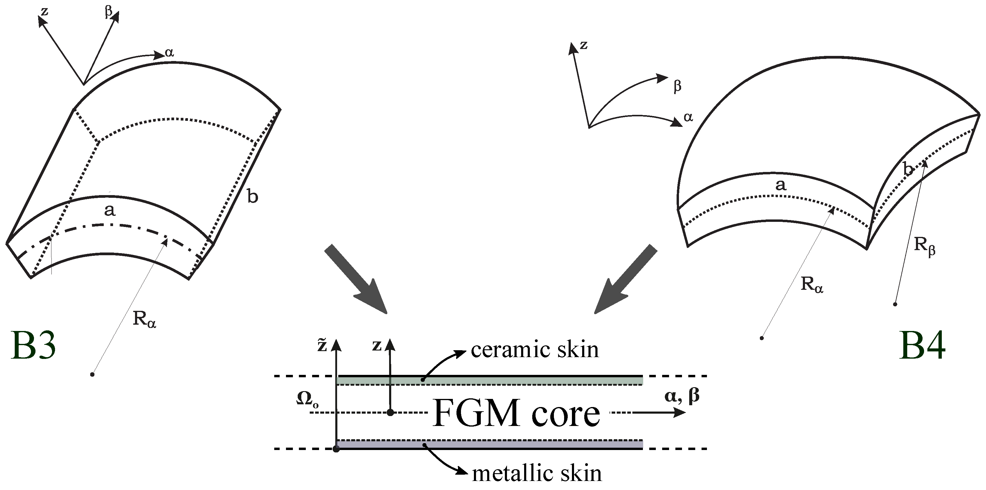
3. 3D Exact Shell Model for Hygro-Elastic Stress Analysis

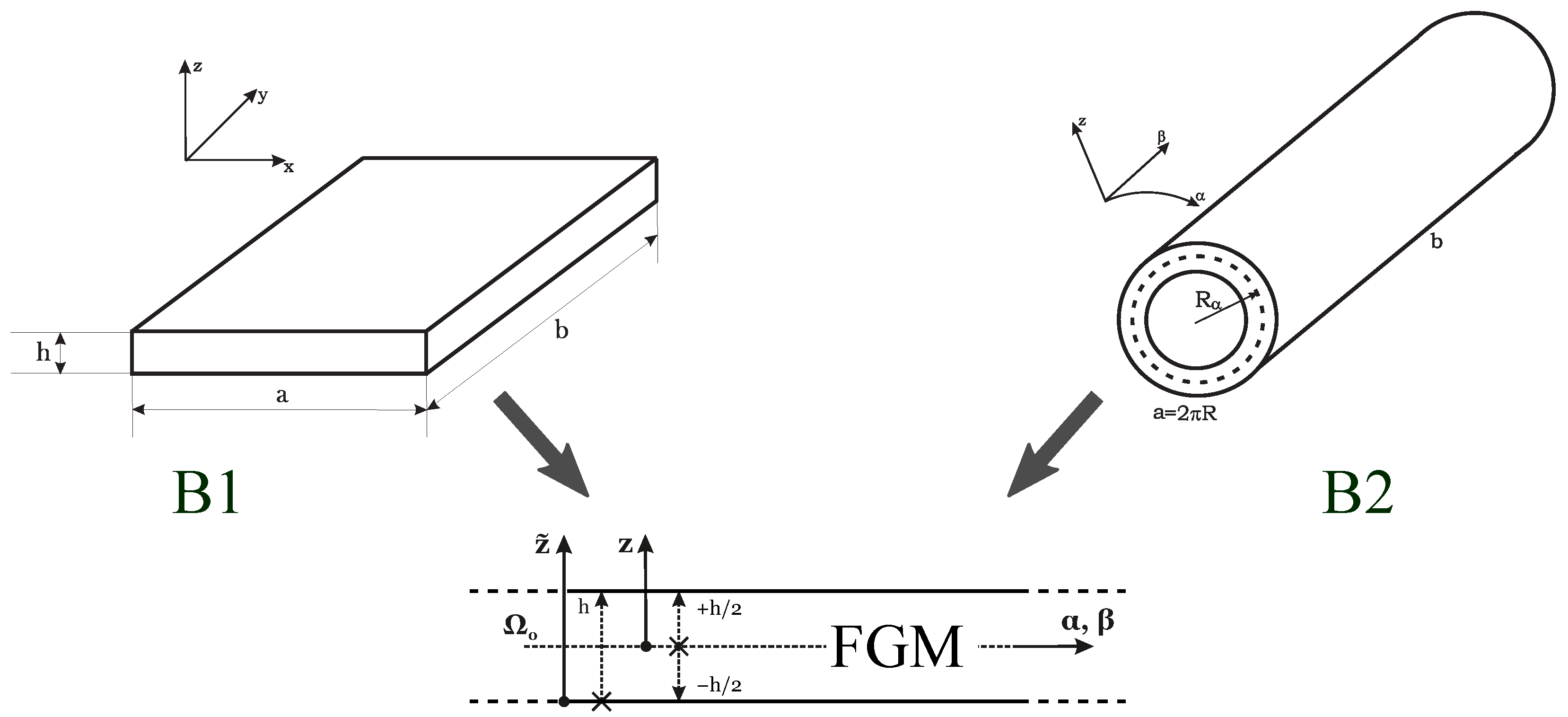
The 3D equilibrium equations for shells are written in the orthogonal mixed curvilinear coordinate system $(\alpha ,\beta ,z)$ shown in Figure 1 and Figure 2. These equations are modified using 3D constitutive equations for Functionally Graded Materials (FGMs) and general geometrical relations for shells in $(\alpha ,\beta ,z)$ coordinates. Therefore, the system includes three differential equations of second order in z, and the related coefficients are not constant because of the radii of curvature and elastic coefficients for FGMs. A reasonable number of mathematical layers is introduced to obtain constant-coefficient equations; redoubling the number of variables allows reducing the order of the differential equations. Simply-supported sides and harmonic variables allow the analytical calculation of the partial derivatives in $\alpha$ and $\beta$ directions. The final system, including the moisture content profile, has only first-order partial derivatives in z, and the exponential matrix method allows determining both general and particular solutions.

The investigated multilayered shells and plates subjected to a moisture content $\mathcal{M}(\alpha ,\beta ,z)$ at the external surfaces have k classical/composite layers and/or functionally graded material layers. Stains defined in an orthogonal mixed curvilinear reference system ($\alpha$,$\beta$,z) are the algebraic summation of mechanical elastic parts (subscript m) and hygroscopic parts (subscript $\mathcal{M}$). The $6\times 1$ vector (${ϵ}_{\alpha \alpha }^k,{ϵ}_{\beta \beta }^k,{ϵ}_{zz}^k,{\gamma }_{\beta z}^k,{\gamma }_{\alpha z}^k,{\gamma }_{\alpha \beta }^k$) for each k layer is defined as

$$\begin{array}{}\mathrm{(25)}& \begin{array}{cc}\hfill {ϵ}_{\alpha \alpha }^k& ={ϵ}_{\alpha \alpha m}^k-{ϵ}_{\alpha \alpha \mathcal{M}}^k=\frac{1}{H_{\alpha }\left(z\right)}\frac{\partial u^k}{\partial \alpha }+\frac{w^k}{H_{\alpha }\left(z\right)R_{\alpha }}-{\eta }_{\alpha }^k\left(z\right){\mathcal{M}}^k,\hfill \end{array}\mathrm{(26)}& \begin{array}{cc}\hfill {ϵ}_{\beta \beta }^k& ={ϵ}_{\beta \beta m}^k-{ϵ}_{\beta \beta \mathcal{M}}^k=\frac{1}{H_{\beta }\left(z\right)}\frac{\partial v^k}{\partial \beta }+\frac{w^k}{H_{\beta }\left(z\right)R_{\beta }}-{\eta }_{\beta }^k\left(z\right){\mathcal{M}}^k,\hfill \end{array}\mathrm{(27)}& \begin{array}{cc}\hfill {ϵ}_{zz}^k& ={ϵ}_{zzm}^k-{ϵ}_{zz\mathcal{M}}^k=\frac{\partial w^k}{\partial z}-{\eta }_z^k\left(z\right){\mathcal{M}}^k,\hfill \end{array}\mathrm{(28)}& \begin{array}{cc}\hfill {\gamma }_{\beta z}^k& ={\gamma }_{\beta zm}^k=\frac{1}{H_{\beta }\left(z\right)}\frac{\partial w^k}{\partial \beta }+\frac{\partial v^k}{\partial z}-\frac{v^k}{H_{\beta }\left(z\right)R_{\beta }},\hfill \end{array}\mathrm{(29)}& \begin{array}{cc}\hfill {\gamma }_{\alpha z}^k& ={\gamma }_{\alpha zm}^k=\frac{1}{H_{\alpha }\left(z\right)}\frac{\partial w^k}{\partial \alpha }+\frac{\partial u^k}{\partial z}-\frac{u^k}{H_{\alpha }\left(z\right)R_{\alpha }},\hfill \end{array}\mathrm{(30)}& \begin{array}{cc}\hfill {\gamma }_{\alpha \beta }^k& ={\gamma }_{\alpha \beta m}^k=\frac{1}{H_{\alpha }\left(z\right)}\frac{\partial v^k}{\partial \alpha }+\frac{1}{H_{\beta }\left(z\right)}\frac{\partial u^k}{\partial \beta },\hfill \end{array}\end{array}$$

In the hygro-elastic strains, the three displacement components $u^k$, $v^k$, and $w^k$ and the scalar moisture content ${\mathcal{M}}^k$ are defined in the reference system ($\alpha$, $\beta$, z). Moisture expansion coefficients ${\eta }_{\alpha }^k\left(z\right)$, ${\eta }_{\beta }^k\left(z\right)$ and ${\eta }_z^k\left(z\right)$ in the k physical layer could depend on the z coordinate in the case of Functionally Graded Material (FGM) layers; they are defined in the structural reference system ($\alpha$, $\beta$, z) starting from the moisture expansion coefficients ${\eta }_1^k\left(z\right)$, ${\eta }_2^k\left(z\right)$ and ${\eta }_3^k\left(z\right)$ in the material reference system (1, 2, 3). The partial derivatives are defined via the symbol ∂.

As anticipated, an essential hypothesis for exact closed-form solutions is the harmonic forms for all the variables: displacement components and moisture content. While the latter has already been discussed, for the displacement components it holds that

$$\begin{array}{cc}\hfill u^k(\alpha ,\beta ,z)& =U^k\left(z\right)cos\left(\overline{\alpha }\alpha \right)sin\left(\overline{\beta }\beta \right),\hfill \end{array}$$

(31)

$$\begin{array}{cc}\hfill v^k(\alpha ,\beta ,z)& =V^k\left(z\right)sin\left(\overline{\alpha }\alpha \right)cos\left(\overline{\beta }\beta \right),\hfill \end{array}$$

(32)

$$\begin{array}{cc}\hfill w^k(\alpha ,\beta ,z)& =W^k\left(z\right)sin\left(\overline{\alpha }\alpha \right)sin\left(\overline{\beta }\beta \right),\hfill \end{array}$$

(33)

displacement amplitudes are indicated as $(U^k\left(z\right),V^k\left(z\right),W^k\left(z\right))$. As already described, m and n are the half-wave numbers, a and b the mid-surface dimensions, and $\overline{\alpha }=\frac{m\pi }{a}$ and $\overline{\beta }=\frac{n\pi }{b}$.

The three-dimensional equilibrium equations for spherical shells having constant radii of curvature $R_{\alpha }=R_{\beta }$ and a total number $N_L$ of physical k (either classical or FGM) layers are

$$\begin{array}{cc}\hfill & H_{\beta }\left(z\right)\frac{\partial {\sigma }_{\alpha \alpha }^k}{\partial \alpha }+H_{\alpha }\left(z\right)\frac{\partial {\sigma }_{\alpha \beta }^k}{\partial \beta }+H_{\alpha }\left(z\right)H_{\beta }\left(z\right)\frac{\partial {\sigma }_{\alpha z}^k}{\partial z}+(\frac{2H_{\beta }\left(z\right)}{R_{\alpha }}+\frac{H_{\alpha }\left(z\right)}{R_{\beta }}){\sigma }_{\alpha z}^k=0,\hfill \end{array}$$

(34)

$$\begin{array}{cc}\hfill & H_{\beta }\left(z\right)\frac{\partial {\sigma }_{\alpha \beta }^k}{\partial \alpha }+H_{\alpha }\left(z\right)\frac{\partial {\sigma }_{\beta \beta }^k}{\partial \beta }+H_{\alpha }\left(z\right)H_{\beta }\left(z\right)\frac{\partial {\sigma }_{\beta z}^k}{\partial z}+(\frac{2H_{\alpha }\left(z\right)}{R_{\beta }}+\frac{H_{\beta }\left(z\right)}{R_{\alpha }}){\sigma }_{\beta z}^k=0,\hfill \end{array}$$

(35)

$$H_{\beta }\left(z\right)\frac{\partial {\sigma }_{\alpha z}^k}{\partial \alpha }+H_{\alpha }\left(z\right)\frac{\partial {\sigma }_{\beta z}^k}{\partial \beta }+H_{\alpha }\left(z\right)H_{\beta }\left(z\right)\frac{\partial {\sigma }_{zz}^k}{\partial z}-\frac{H_{\beta }\left(z\right)}{R_{\alpha }}{\sigma }_{\alpha \alpha }^k-\frac{H_{\alpha }\left(z\right)}{R_{\beta }}{\sigma }_{\beta \beta }^k+(\frac{H_{\beta }\left(z\right)}{R_{\alpha }}+\frac{H_{\alpha }\left(z\right)}{R_{\beta }}){\sigma }_{zz}^k=0.$$

(36)

Three-dimensional equilibrium equations for cylinders/cylindrical panels and plates are obtained from Equations (34)–(36) when one of the two radii of curvature is infinite and when both the radii of curvature are infinite, respectively.

The constitutive equations are developed by considering the algebraic summation of mechanical elastic strains and hygroscopic strains:

$${\sigma }^k={\mathit{C}}^k\left(z\right){ϵ}^k={\mathit{C}}^k\left(z\right)({ϵ}_m^k-{ϵ}_{\mathcal{M}}^k),$$

(37)

${\sigma }^k$ is the stress vector having a $6\times 1$ dimension, ${\mathit{C}}^k\left(z\right)$ is the $6\times 6$ elastic coefficient matrix and it could depend on the z coordinate in the case of a kth FGM layer. The strains are included in the constitutive equations by using the form shown in Equations (25)–(30). Closed-form solutions are possible when orthotropic angles are $0^{\circ }$ or ${90}^{\circ }$ to obtain $C_{16}^k\left(z\right)=C_{26}^k\left(z\right)=C_{36}^k\left(z\right)=C_{45}^k\left(z\right)=0$ in the structural reference system ($\alpha$, $\beta$, z). Therefore,

$${\mathbf{C}}^k\left(z\right)=\left[\begin{array}{cccccc}{C}_{11}^k\left(z\right)& C_{12}^k\left(z\right)& C_{13}^k\left(z\right)& 0& 0& 0\\ C_{12}^k\left(z\right)& C_{22}^k\left(z\right)& C_{23}^k\left(z\right)& 0& 0& 0\\ C_{13}^k\left(z\right)& C_{23}^k\left(z\right)& C_{33}^k\left(z\right)& 0& 0& 0\\ 0& 0& 0& C_{44}^k\left(z\right)& 0& 0\\ 0& 0& 0& 0& C_{55}^k\left(z\right)& 0\\ 0& 0& 0& 0& 0& C_{66}^k\left(z\right)\end{array}\right].$$

(38)

The explicit form of the constitutive equations develops thanks to the introduction of the geometrical Equations (25)–(30) into the constitutive Equation (37):

$$\begin{array}{}\mathrm{(39)}& \begin{array}{cc}\hfill {\sigma }_{\alpha \alpha }^k& =\frac{C_{11}^k\left(z\right)}{H_{\alpha }\left(z\right)}{u}_{,\alpha }^k+\frac{C_{11}^k\left(z\right)}{H_{\alpha }\left(z\right)R_{\alpha }}{w}^k+\frac{C_{12}^k\left(z\right)}{H_{\beta }\left(z\right)}{v}_{,\beta }^k+\frac{C_{12}^k\left(z\right)}{H_{\beta }\left(z\right)R_{\beta }}{w}^k+C_{13}^k\left(z\right)w_{,z}^k-{\xi }_{\alpha }^k\left(z\right){\mathcal{M}}^k,\hfill \end{array}\mathrm{(40)}& \begin{array}{cc}\hfill {\sigma }_{\beta \beta }^k& =\frac{C_{12}^k\left(z\right)}{H_{\alpha }\left(z\right)}{u}_{,\alpha }^k+\frac{C_{12}^k\left(z\right)}{H_{\alpha }\left(z\right)R_{\alpha }}{w}^k+\frac{C_{22}^k\left(z\right)}{H_{\beta }\left(z\right)}{v}_{,\beta }^k+\frac{C_{22}^k\left(z\right)}{H_{\beta }\left(z\right)R_{\beta }}{w}^k+C_{23}^k\left(z\right)w_{,z}^k-{\xi }_{\beta }^k\left(z\right){\mathcal{M}}^k,\hfill \end{array}\mathrm{(41)}& \begin{array}{cc}\hfill {\sigma }_{zz}^k& =\frac{C_{13}^k\left(z\right)}{H_{\alpha }\left(z\right)}{u}_{,\alpha }^k+\frac{C_{13}^k\left(z\right)}{H_{\alpha }\left(z\right)R_{\alpha }}{w}^k+\frac{C_{23}^k\left(z\right)}{H_{\beta }\left(z\right)}{v}_{,\beta }^k+\frac{C_{23}^k\left(z\right)}{H_{\beta }\left(z\right)R_{\beta }}{w}^k+C_{33}^k\left(z\right)w_{,z}^k-{\xi }_z^k\left(z\right){\mathcal{M}}^k,\hfill \end{array}\mathrm{(42)}& \begin{array}{cc}\hfill {\sigma }_{\beta z}^k& =\frac{C_{44}^k\left(z\right)}{H_{\beta }\left(z\right)}{w}_{,\beta }^k+C_{44}^k\left(z\right)v_{,z}^k-\frac{C_{44}^k\left(z\right)}{H_{\beta }\left(z\right)R_{\beta }}{v}^k,\hfill \end{array}\mathrm{(43)}& \begin{array}{cc}\hfill {\sigma }_{\alpha z}^k& =\frac{C_{55}^k\left(z\right)}{H_{\alpha }\left(z\right)}{w}_{,\alpha }^k+C_{55}^k\left(z\right)u_{,z}^k-\frac{C_{55}^k\left(z\right)}{H_{\alpha }\left(z\right)R_{\alpha }}{u}^k,\hfill \end{array}\mathrm{(44)}& \begin{array}{cc}\hfill {\sigma }_{\alpha \beta }^k& =\frac{C_{66}^k\left(z\right)}{H_{\alpha }\left(z\right)}{v}_{,\alpha }^k+\frac{C_{66}^k\left(z\right)}{H_{\beta }\left(z\right)}{u}_{,\beta }^k,\hfill \end{array}\end{array}$$

partial derivatives ($\frac{\partial }{\partial \alpha }$), ($\frac{\partial }{\partial \beta }$), and ($\frac{\partial }{\partial z}$) are indicated in Equations (39)–(44) through subscripts ($,\alpha$), ($,\beta$), and ($,z$), respectively. Terms ${\xi }_{\alpha }^k\left(z\right)$, ${\xi }_{\beta }^k\left(z\right)$, and ${\xi }_z^k\left(z\right)$ designate the hygro-mechanical coupling coefficients in the structural reference system ($\alpha$, $\beta$, z), and they could depend on z in the case of FGM layers:

$$\begin{array}{c}\hfill {\xi }_{\alpha }^k\left(z\right)=C_{11}^k\left(z\right){\eta }_{\alpha }^k\left(z\right)+C_{12}^k\left(z\right){\eta }_{\beta }^k\left(z\right)+C_{13}^k\left(z\right){\eta }_z^k\left(z\right),\end{array}$$

(45)

$$\begin{array}{c}\hfill {\xi }_{\beta }^k\left(z\right)=C_{12}^k\left(z\right){\eta }_{\alpha }^k\left(z\right)+C_{22}^k\left(z\right){\eta }_{\beta }^k\left(z\right)+C_{23}^k\left(z\right){\eta }_z^k\left(z\right),\end{array}$$

(46)

$$\begin{array}{c}\hfill {\xi }_z^k\left(z\right)=C_{13}^k\left(z\right){\eta }_{\alpha }^k\left(z\right)+C_{23}^k\left(z\right){\eta }_{\beta }^k\left(z\right)+C_{33}^k\left(z\right){\eta }_z^k\left(z\right).\end{array}$$

(47)

The final system is obtained thanks to the substitution of the harmonic form equations for displacements and moisture content Equations (1)–(31) and the modified constitutive relations Equations (39)–(44) into the three-dimensional equilibrium Equations (34)–(36) developed for spherical shells:

$$\begin{array}{}\mathrm{(48)}& \begin{array}{cc}\hfill & A_1^j{U}^j+A_2^j{V}^j+A_3^j{W}^j+A_4^j{U}_{,z}^j+A_5^j{W}_{,z}^j+A_6^j{U}_{,zz}^j+L_1^j{M}^j=0,\hfill \end{array}\mathrm{(49)}& \begin{array}{cc}\hfill & A_7^j{U}^j+A_8^j{V}^j+A_9^j{W}^j+A_{10}^j{V}_{,z}^j+A_{11}^j{W}_{,z}^j+A_{12}^j{V}_{,zz}^j+L_2^j{M}^j=0,\hfill \end{array}\mathrm{(50)}& \begin{array}{cc}\hfill & A_{13}^j{U}^j+A_{14}^j{V}^j+A_{15}^j{W}^j+A_{16}^j{U}_{,z}^j+A_{17}^j{V}_{,z}^j+A_{18}^j{W}_{,z}^j+A_{19}^j{W}_{,zz}^j+L_3^j{M}_{,z}^j+L_4^j{M}^j=0.\hfill \end{array}\end{array}$$

The above equations have no constant coefficients because the parametric coefficients $H_{\alpha }$ and $H_{\beta }$ depend on z in the case of shell geometries and/or elastic and hygrometric coefficients depend on z in FGM layers. For these reasons, each k physical layer is divided into a suitable number of mathematical layers indicated with a new index j which changes from 1 to the global number of mathematical layers G. In each j mathematical layer, the parametric coefficients $H_{\alpha }$ and $H_{\beta }$ and the variable elastic and hygrometric coefficients for FGM layers can be exactly defined by using the z coordinate in the middle of each j layer. Therefore, coefficients $A_s^j$ (s from 1 to 19) and $L_r^j$ (r from 1 to 4) become constant terms in the compact form of the system of differential equations in z defined in Equations (48)–(50).

Equations (48)–(50) indicate a system of three differential equations of second order in z. The unknowns are the displacement and moisture content amplitudes and the associated derivatives calculated to z. The derivatives in $\alpha$ and $\beta$ have already been calculated via the harmonic forms for displacements and moisture content previously introduced. In this system, decoupling the variables is possible: this means a separate quantification of the moisture content profile through the thickness direction z, addressed in an appropriate section. Therefore, it becomes a known term.

The consequence of these choices is that the system contains second-order differential equations only, in the displacement amplitudes $U^j$, $V^j$, $W^j$ and their derivatives in z. Redoubling the variables as proposed in [71,72] allows reducing the system into a first-order one in z. In each j layer, the $3\times 1$ vector of unknowns ($U^j$, $V^j$, $W^j$) becomes a $6\times 1$ unknown vector ($U^j$, $V^j$, $W^j$, $U^{j^{{}^{\prime }}}$, $V^{j^{{}^{\prime }}}$, $W^{j^{{}^{\prime }}}$); superscript ${}^{\prime }$ indicates derivatives performed to z (also written as $\frac{\partial }{\partial z}$). Terms $M^j$ and $M^{j^{\prime }}$ can be considered as known terms because they can be opportunely calculated, as will be demonstrated in the next section:

$$\begin{array}{cc}\hfill & \left[\begin{array}{cccccc}{A}_6^j& 0& 0& 0& 0& 0\\ 0& A_{12}^j& 0& 0& 0& 0\\ 0& 0& A_{19}^j& 0& 0& 0\\ 0& 0& 0& A_6^j& 0& 0\\ 0& 0& 0& 0& A_{12}^j& 0\\ 0& 0& 0& 0& 0& A_{19}^j\end{array}\right]{\left[\begin{array}{c}{U}^j\\ V^j\\ W^j\\ U^{j^{{}^{\prime }}}\\ V^{j^{{}^{\prime }}}\\ W^{j^{{}^{\prime }}}\end{array}\right]}^{{}^{\prime }}=\hfill \\ \hfill & \left[\begin{array}{cccccc}0& 0& 0& A_6^j& 0& 0\\ 0& 0& 0& 0& A_{12}^j& 0\\ 0& 0& 0& 0& 0& A_{19}^j\\ -A_1^j& -A_2^j& -A_3^j& -A_4^j& 0& -A_5^j\\ -A_7^j& -A_8^j& -A_9^j& 0& -A_{10}^j& -A_{11}^j\\ -A_{13}^j& -A_{14}^j& -A_{15}^j& -A_{16}^j& -A_{17}^j& -A_{18}^j\end{array}\right]\left[\begin{array}{c}{U}^j\\ V^j\\ W^j\\ U^{j^{{}^{\prime }}}\\ V^{j^{{}^{\prime }}}\\ W^{j^{{}^{\prime }}}\end{array}\right]+\left[\begin{array}{cccccc}0& 0& 0& 0& 0& 0\\ 0& 0& 0& 0& 0& 0\\ 0& 0& 0& 0& 0& 0\\ -L_1^j& 0& 0& 0& 0& 0\\ -L_2^j& 0& 0& 0& 0& 0\\ -L_4^j& -L_3^j& 0& 0& 0& 0\end{array}\right]\left[\begin{array}{c}{M}^j\\ M^{j^{{}^{\prime }}}\\ 0\\ 0\\ 0\\ 0\end{array}\right],\hfill \end{array}$$

(51)

By defining vectors ${\mathit{U}}^j={\left[U^j{V}^j{W}^j{U}^{j^{{}^{\prime }}}{V}^{j^{{}^{\prime }}}{W}^{j^{{}^{\prime }}}\right]}^T$, ${{\mathit{U}}^j}^{{}^{\prime }}=\frac{\partial {\mathit{U}}^j}{\partial z}$ and ${\mathit{M}}^j$$={\left[M^j{M}^{j^{{}^{\prime }}}0000\right]}^T$ (where T means the transpose of a vector), the following compact form is possible:

$${\mathit{D}}^j{{\mathit{U}}^j}^{{}^{\prime }}={\mathit{A}}^j{\mathit{U}}^j+{\mathit{L}}^j{\mathit{M}}^j,$$

(52)

the above equation, thanks to the definitions ${\mathit{A}}^{{*}^j}={\mathit{D}}^{j^{-1}}{\mathit{A}}^j$ and ${\mathit{L}}^{{*}^j}={\mathit{D}}^{j^{-1}}{\mathit{L}}^j$, can be rewritten as

$${{\mathit{U}}^j}^{{}^{\prime }}={\mathit{D}}^{j^{-1}}{\mathit{A}}^j{\mathit{U}}^j+{\mathit{D}}^{j^{-1}}{\mathit{L}}^j{\mathit{M}}^j,$$

(53)

$${{\mathit{U}}^j}^{{}^{\prime }}={\mathit{A}}^{{*}^j}{\mathit{U}}^j+{\mathit{L}}^{{*}^j}{\mathit{M}}^j.$$

(54)

The moisture content profile through the thickness direction z can be calculated using one of the three methods proposed in the previous section. This profile can be reconstructed using a linear approximation of the moisture content in each j mathematical layer. This reconstruction can be defined as

$$M^j\left({\tilde{z}}^j\right)=a_M^j{\tilde{z}}^j+b_M^j,$$

(55)

in a jth mathematical layer, $a_M^j$ and $b_M^j$ are two constant coefficients. The first represents the slope of the moisture content profile inside a mathematical layer; the second the moisture content at the bottom. ${\tilde{z}}^j$ is a local thickness coordinate for each j mathematical layer, and it changes from 0 at the bottom of the considered j mathematical layer to the top value $h^j$ of the same mathematical layer.

The system of first-order differential equations in $\tilde{z}$ or z shown in Equation (54) is not homogeneous because the hygroscopic term ${\mathit{L}}^{{*}^j}{\mathit{M}}^j$ depends on ${\tilde{z}}^j$ or $z^j$. In the case of a generic system of non-homogeneous first-order differential equations having an unknown $G\times 1$ vector $\mathit{x}$, a $G\times G$ |$\mathit{A}$ matrix containing constant coefficients, and a known function vector $\mathit{f}\left(t\right)={[f_1\left(t\right)...f_G\left(t\right)]}^T$,we can write

$$\frac{\mathrm{d}\mathit{x}}{\mathrm{d}t}=\mathit{A}\mathit{x}+\mathit{f}\left(t\right),$$

(56)

a possible solution of the Equation (56) can be obtained via the exponential matrix method:

$$\mathit{x}\left(t\right)={\mathrm{e}}^{\mathit{A}(t-t_0)}{\mathit{x}}_0+{\int }_{t_0}^t{\mathrm{e}}^{\mathit{A}(t-s)}\mathit{f}\left(s\right)ds.$$

(57)

The known term in Equation (54) can be given in the following complete form:

$${\mathit{M}}^{{*}^j}={\mathit{L}}^{{*}^j}{\mathit{M}}^j=\left[\begin{array}{cccccc}0& 0& 0& 0& 0& 0\\ 0& 0& 0& 0& 0& 0\\ 0& 0& 0& 0& 0& 0\\ -L_1^{{*}^j}& 0& 0& 0& 0& 0\\ -L_2^{{*}^j}& 0& 0& 0& 0& 0\\ -L_4^{{*}^j}& -L_3^{{*}^j}& 0& 0& 0& 0\end{array}\right]\left[\begin{array}{c}{a}_M^j{\tilde{z}}^j+b_M^j\\ a_M^j\\ 0\\ 0\\ 0\\ 0\end{array}\right]=\left[\begin{array}{c}0\\ 0\\ 0\\ -L_1^{{*}^j}(a_M^j{\tilde{z}}^j+b_M^j)\\ -L_2^{{*}^j}(a_M^j{\tilde{z}}^j+b_M^j)\\ -L_4^{{*}^j}(a_M^j{\tilde{z}}^j+b_M^j)-L_3^{{*}^j}{a}_M^j\end{array}\right].$$

(58)

Therefore, Equation (54) can be rewritten as

$${{\mathit{U}}^j}^{{}^{\prime }}={\mathit{A}}^{{*}^j}{\mathit{U}}^j+{\mathit{M}}^{{*}^j},$$

(59)

${\mathit{M}}^{{*}^j}$ includes only linear and known functions in ${\tilde{z}}^j$ coordinate. The Equation (59) can be solved through the exponential matrix method:

$${\mathit{U}}^j\left({\tilde{z}}^j\right)={\mathrm{e}}^{\left({\mathit{A}}^{{*}^j}{\tilde{z}}^j\right)}{\mathit{U}}^j\left(0\right)+{\int }_0^{{\tilde{z}}^j}{\mathrm{e}}^{\left({\mathit{A}}^{{*}^j}({\tilde{z}}^j-s)\right)}{\mathit{M}}^{{*}^j}\left(s\right)ds.$$

(60)

${\mathit{A}}^{{**}^j}={\mathrm{e}}^{\left({\mathit{A}}^{{*}^j}{h}^j\right)}$ and ${\mathit{L}}^{{**}^j}={\int }_0^{h^j}{\mathrm{e}}^{\left({\mathit{A}}^{{*}^j}(h^j-s)\right)}{\mathit{M}}^{{*}^j}\left(s\right)ds$ must be opportunely defined for each j layer having thickness $h^j$. In this way, the displacement vector at the top of each j mathematical layer is calculated. Both terms are defined via the exponential matrix opportunely expanded and evaluated in each j mathematical layer with thickness $h^j$:

$${\mathit{A}}^{{**}^j}={\mathrm{e}}^{\left({\mathit{A}}^{{*}^j}{h}^j\right)}=\mathit{I}+{\mathit{A}}^{{*}^j}{h}^j+\frac{{{\mathit{A}}^{{*}^j}}^2}{2!}{h^j}^2+\frac{{{\mathit{A}}^{{*}^j}}^3}{3!}{h^j}^3+\cdots +\frac{{{\mathit{A}}^{{*}^j}}^N}{N!}{h^j}^N,$$

(61)

$$\begin{array}{cc}\hfill {\mathit{L}}^{{**}^j}=& {\int }_0^{h^j}{\mathrm{e}}^{\left({\mathit{A}}^{{*}^j}(h^j-s)\right)}{\mathit{M}}^{{*}^j}\left(s\right)ds={\int }_0^{h^j}(\mathit{I}+{\mathit{A}}^{{*}^j}(h^j-s)+\frac{{{\mathit{A}}^{{*}^j}}^2}{2!}{(h^j-s)}^2+\frac{{{\mathit{A}}^{{*}^j}}^3}{3!}{(h^j-s)}^3+\hfill \\ & \cdots +\frac{{{\mathit{A}}^{{*}^j}}^N}{N!}{(h^j-s)}^N){\mathit{M}}^{{*}^j}\left(s\right)ds,\hfill \end{array}$$

(62)

where $\mathit{I}$ is the $6\times 6$ identity matrix, and the integral given in Equation (60) can be calculated in each j layer having thickness $h^j$ by using the exponential matrix and the same order N already shown in Equation (61). By using Equations (61) and (62), Equation (60) is modified as

$${\mathit{U}}^j\left(h^j\right)={\mathit{A}}^{{**}^j}{\mathit{U}}^j\left(0\right)+{\mathit{L}}^{{**}^j},$$

(63)

where ${\mathit{U}}_t^j$ indicates ${\mathit{U}}^j\left(h^j\right)$ and it is defined at the top t of each j layer, and ${\mathit{U}}_b^j$ indicates ${\mathit{U}}^j\left(0\right)$ and it is defined at the bottom of each j layer. In this way, Equation (63) is defined as

$${\mathit{U}}_t^j={\mathit{A}}^{{**}^j}{\mathit{U}}_b^j+{\mathit{L}}^{{**}^j}.$$

(64)

Using Equation (64) allows to connect displacements and their derivatives in z defined at the top of the j mathematical layer with the same variables defined at the bottom of the same j layer.

The general three-dimensional shell model is developed using a layer-wise approach. Inter-laminar continuity conditions in displacements and transverse stresses must be defined at each interface between the two adjacent mathematical layers. The inter-laminar continuity conditions for displacements come through congruence hypotheses:

$$u_b^j=u_t^{j-1},v_b^j=v_t^{j-1},w_b^j=w_t^{j-1}.$$

(65)

The inter-laminar continuity conditions for transverse shear and normal transverse stresses are defined employing equilibrium hypotheses:

$${\sigma }_{z{z}_b}^j={\sigma }_{z{z}_t}^{j-1},{\sigma }_{\alpha z_b}^j={\sigma }_{\alpha z_t}^{j-1},{\sigma }_{\beta z_b}^j={\sigma }_{\beta z_t}^{j-1}.$$

(66)

The formulation of this solution requires rewriting the inter-laminar continuity conditions, Equations (65) and (66), in a displacement form. Achieving this task is possible by recalling the constitutive Equations (39)–(44) and the harmonic form of the variables of the problem, Equations (1) and (31)–(33). This procedure allows writing the inter-laminar continuity condition in the amplitude displacements and their derivatives to the thickness coordinate. Then, compacting the notation is possible, recalling the vectors ${\mathit{U}}^j$ and ${\mathit{M}}^j$, and introducing a pair of transfer matrices. The procedure is similar to that employed in [25]; exception made for an additional coefficient multiplying the moisture content amplitude:

$${\left[\begin{array}{c}U\\ V\\ W\\ U^{{}^{\prime }}\\ V^{{}^{\prime }}\\ W^{{}^{\prime }}\end{array}\right]}_b^j={\left[\begin{array}{cccccc}1& 0& 0& 0& 0& 0\\ 0& 1& 0& 0& 0& 0\\ 0& 0& 1& 0& 0& 0\\ T_1& 0& T_2& T_3& 0& 0\\ 0& T_4& T_5& 0& T_6& 0\\ T_7& T_8& T_9& 0& 0& T_{10}\end{array}\right]}^{j-1,j}{\left[\begin{array}{c}U\\ V\\ W\\ U^{{}^{\prime }}\\ V^{{}^{\prime }}\\ W^{{}^{\prime }}\end{array}\right]}_t^{j-1}+{\left[\begin{array}{cccccc}0& 0& 0& 0& 0& 0\\ 0& 0& 0& 0& 0& 0\\ 0& 0& 0& 0& 0& 0\\ 0& 0& 0& 0& 0& 0\\ 0& 0& 0& 0& 0& 0\\ T_{11}& 0& 0& 0& 0& 0\end{array}\right]}^{j-1,j}{\left[\begin{array}{c}M\\ M^{{}^{\prime }}\\ 0\\ 0\\ 0\\ 0\end{array}\right]}_t^{j-1}.$$

(67)

The first three rows of Equation (67) denote the displacement continuity equations; the last three are the continuity conditions for stresses. The compact form of Equation (67) follows:

$${\mathit{U}}_b^j={\mathit{T}}_U^{j-1,j}{\mathit{U}}_t^{j-1}+{\mathit{T}}_M^{j-1,j}{\mathit{M}}_t^{j-1}.$$

(68)

Equation (68) expresses the link between the displacements and their z derivatives, calculated at the bottom of the jth layer, with their corresponding values plus the moisture content (and its z derivative), at the top of the ($j-1$)th layer.

The harmonic form implemented in all the variables of the problem automatically satisfies the simply supported boundary conditions, here reported for exhaustiveness:

$$\begin{array}{cc}\hfill & w=v=0,{\sigma }_{\alpha \alpha }=0\mathrm{for}\alpha =0,a,\hfill \end{array}$$

(69)

$$\begin{array}{cc}\hfill & w=u=0,{\sigma }_{\beta \beta }=0\mathrm{for}\beta =0,b\hfill \end{array}$$

(70)

This solution extends the model already seen in [25] for the static analysis of shells subjected to static loads. In that context, mechanical loads can act on the external top and bottom surfaces, with components defined in the three directions $\alpha$, $\beta$, and z. They are grouped into vectors $\mathit{P}={\left(P_{\alpha }{P}_{\beta }{P}_z\right)}^T$; the superscript G means the one acting on the top surface; the one with superscript 1 identifies the one acting on the lower one. The effect of the external loads affects the displacements:

$$\begin{array}{cc}\hfill & {\mathit{B}}_t^G{\mathit{U}}_t^G={\mathit{P}}_t^G,\hfill \end{array}$$

(71)

$$\begin{array}{cc}\hfill & {\mathit{B}}_b^1{\mathit{U}}_b^1={\mathit{P}}_b^1,\hfill \end{array}$$

(72)

more details are available in [25]. The hygro-elastic analysis does not involve anything different; once applied, the moisture content induces an equivalent load, which sums up the (possible) mechanical load. The matrices $\mathit{B}$ convert the mechanical and/or hygrometric loads into displacements. ${\mathit{B}}_t^G$, in Equation (71) handles the top (t) of the last layer (G); ${\mathit{B}}_b^1$, in Equation (72), the bottom (b) of the first layer (1).

The algebraic system of Equations (71) and (72) can be reformulated into a matrix form, rewriting the displacements ${\mathit{U}}_t^G={\mathit{U}}^G\left(h^G\right)$ as a function of ${\mathit{U}}_b^1={\mathit{U}}^1\left(0\right)$. This rewriting is possible through a recursive substitution of Equation (68) into Equation (64), linking the displacements at the top of the last layer (and their z derivatives) to those at the bottom of the first layer:

$$\begin{array}{cc}\hfill {\mathit{U}}_t^G=& \left({{\mathit{A}}^{**}}^G{\mathit{T}}_U^{G-1,G}{{\mathit{A}}^{**}}^{G-1}{\mathit{T}}_U^{G-2,G-1}......{{\mathit{A}}^{**}}^2{\mathit{T}}_U^{1,2}{{\mathit{A}}^{**}}^1\right){\mathit{U}}_b^1+\hfill \\ \hfill & ({{\mathit{A}}^{**}}^G{\mathit{T}}_U^{G-1,G}{{\mathit{A}}^{**}}^{G-1}......{{\mathit{A}}^{**}}^2{\mathit{T}}_U^{1,2}{{\mathit{L}}^{**}}^1+\hfill \\ \hfill & {{\mathit{A}}^{**}}^G{\mathit{T}}_U^{G-1,G}{{\mathit{A}}^{**}}^{G-1}......{{\mathit{A}}^{**}}^3{\mathit{T}}_U^{2,3}{{\mathit{L}}^{**}}^2+\hfill \\ \hfill & ⋮\hfill \\ \hfill & {{\mathit{A}}^{**}}^G{\mathit{T}}_U^{G-1,G}{{\mathit{L}}^{**}}^{G-1}+\hfill \\ \hfill & {{\mathit{L}}^{**}}^G+\hfill \\ \hfill & {{\mathit{A}}^{**}}^G{\mathit{T}}_U^{G-1,G}{{\mathit{A}}^{**}}^G......{{\mathit{A}}^{**}}^2{\mathit{T}}_M^{1,2}{\mathit{M}}_t^1+\hfill \\ \hfill & {{\mathit{A}}^{**}}^G{\mathit{T}}_U^{G-1,G}{{\mathit{A}}^{**}}^G......{{\mathit{A}}^{**}}^3{\mathit{T}}_M^{2,3}{\mathit{M}}_t^2+\hfill \\ \hfill & ⋮\hfill \\ \hfill & {{\mathit{A}}^{**}}^G{\mathit{T}}_U^{G-1,G}{{\mathit{A}}^{**}}^{G-1}{\mathit{T}}_M^{G-2,G-1}{\mathit{M}}_t^{G-2}+\hfill \\ \hfill & {{\mathit{A}}^{**}}^G{\mathit{T}}_M^{G-1,G}{\mathit{M}}_t^{G-1}).\hfill \end{array}$$

(73)

Equation (73) consists of two main blocks. The first has as a common multiplication factor the bottom displacements of the first layer ${\mathit{U}}_b^1$; the content in the brackets is a $6\times 6$ matrix, which is identical to that defined ${\mathit{H}}_m$ for classical elastic analysis in [25]. The hygrometric field brings with it additional terms included in the second block. The terms ${{\mathit{L}}^{**}}^j$ explicitly include the hygrometric profile; they are G as each mathematical layer features its own profile. The terms ${\mathit{M}}_t^j$ set the moisture content at each interface; consequently, they are $G-1$. This block is a known and constant term; it takes the form of a $6\times 1$ vector, from now on referred to as ${\mathit{H}}_M$. Therefore, the compact expression of Equation (73) takes the following form:

$${\mathit{U}}_t^G={\mathit{H}}_m{\mathit{U}}_b^1+{\mathit{H}}_M.$$

(74)

Given this result, Equation (71) can be rewritten in terms of ${\mathit{U}}_b^1$:

$${\mathit{B}}_t^G{\mathit{H}}_m{\mathit{U}}_b^1=-{\mathit{B}}_t^G{\mathit{H}}_M.$$

(75)

Equations (72) and (75) now share the same unknown; they can be put to system as follows:

$$\mathit{E}{\mathit{U}}_b^1={\mathit{P}}_M,$$

(76)

where

$$\mathit{E}=\left[\begin{array}{c}{\mathit{B}}_t^G{\mathit{H}}_m\\ {\mathit{B}}_b^1\end{array}\right]$$

(77)

and

$${\mathit{P}}_M=\left[\begin{array}{c}-{\mathit{B}}_t^G{\mathit{H}}_M\\ \mathit{0}\end{array}\right].$$

(78)

One of the main advantages of this solution is that the dimensions of the matrix $\mathit{E}$ keep low, $6\times 6$, despite the number G of mathematical layers and the layer-wise approach to the problem. Furthermore, $\mathit{E}$ is the same as that needed for the classical elastic analysis (see in [25]). The vector ${\mathit{P}}_M$ adds the hygrometric load as an equivalent mechanical action and sums up the (possible) mechanical load $\mathit{P}$. Solving the system allows getting the bottom displacement components (and their z derivatives); Equations (64) and (68) allow then calculating their values at any coordinate in the thickness direction.

4. Results

This section is of fundamental importance. First of all, it defines the properties of the Functionally Graded (FM) layers, presenting the mechanical and hygrometric properties of their constituents and the law defining their variation in composition. Then, it features two subsections. The first one validates this exact 3D solution for shells embedding layers made of FGM. Validations of new solutions are often conducted comparing the new outputs with those already available in the literature. Besides verifying the accuracy of this solution, this phase helps define how many mathematical layers should be used to consider with confidence the effects of the curvature and those of the FGM law and the order of expansion to use in the exponential matrix calculation. Strengthened by those results, the second subsection presents a set of new results. The effect of the moisture content field is studied on different geometries, featuring different stacking sequences, thickness ratios, and moisture content boundary conditions.

In all the assessments and benchmarks, the FGM layers rely on two constituents: a metal and ceramic. The metal is Monel, 70Ni30Cu, a nickel-based alloy; the ceramic is Zirconia. An estimate of the mechanical properties is given in terms of the bulk modulus K and the shear modulus $\mu$ of the two materials; the moisture expansion coefficients $\eta$ and the moisture diffusion coefficients $\mathcal{D}$ are given explicitly:

$$\begin{array}{cc}\hfill & K_m=227.24\mathrm{GPa},{\mu }_m=65.55\mathrm{GPa},{\eta }_m=2\times {10}^{-3}\frac{1}{\%},{\mathcal{D}}_m={10}^{-9}\frac{\mathrm{kg}}{\mathrm{ms}},\hfill \end{array}$$

(79)

$$\begin{array}{cc}\hfill & K_c=125.83\mathrm{GPa},{\mu }_c=58.077\mathrm{GPa},{\eta }_c=1\times {10}^{-3}\frac{1}{\%},{\mathcal{D}}_c={10}^{-10}\frac{\mathrm{kg}}{\mathrm{ms}},\hfill \end{array}$$

(80)

The metal and the ceramic phases are denoted by the subscripts m and c. The estimate of the thermal properties is also given, as they will be necessary in the assessment phase:

$$\begin{array}{cc}\hfill & {\gamma }_m=15\times {10}^{-6}\frac{1}{K},{\kappa }_m=25\frac{\mathrm{W}}{\mathrm{mK}}\hfill \end{array}$$

(81)

$$\begin{array}{cc}\hfill & {\gamma }_c=10\times {10}^{-6}\frac{1}{K},{\kappa }_c=2.09\frac{\mathrm{W}}{\mathrm{mK}}\hfill \end{array}$$

(82)

$\gamma$ denotes the thermal expansion coefficient, while $\kappa$ the conductivity coefficient. This work assumes that the volume fraction of the ceramic phase follows a power law of order p. Introducing the thickness of the FG layer $h_{{}_{FG}}$ and a local thickness coordinate ${\tilde{z}}_{{}_{FG}}$ inside it (0 at its bottom, h at its top), the FG law takes the following expression:

$$V_c={({\tilde{z}}_{{}_{FG}}/h_{{}_{FG}})}^p$$

(83)

At the bottom of the FG layer, where ${\tilde{z}}_{{}_{FG}}=0$, Equation (83) implies $V_c=0$, meaning that it is made of metal only. At the top of the FG layer, where ${\tilde{z}}_{{}_{FG}}=h_{{}_{FG}}$, Equation (83) implies $V_c=1$, meaning that it is made of ceramic only. The bulk and the shear moduli of the FG layer evolve along with the thickness direction following the Mori–Tanaka estimates:

$$\frac{K-K_m}{K_c-K_m}=\frac{V_c}{1+(1-V_c)\frac{K_c-K_m}{K_m+\frac{4}{3}{\mu }_m}},\frac{\mu -{\mu }_m}{{\mu }_c-{\mu }_m}=\frac{V_c}{1+(1-V_c)\frac{{\mu }_c-{\mu }_m}{{\mu }_m+f_m}},f_m=\frac{{\mu }_m(9K_m+8{\mu }_m)}{6(K_m+2{\mu }_m)}$$

(84)

The same applies to the effective moisture expansion and moisture diffusion coefficients, by analogy with the estimates of Hatta and Taya for the corresponding thermal properties:

$$\frac{\mathcal{D}-{\mathcal{D}}_m}{{\mathcal{D}}_c-{\mathcal{D}}_m}=\frac{V_c}{1+(1-V_c)\frac{{\mathcal{D}}_c-{\mathcal{D}}_m}{3{\mathcal{D}}_m}},\frac{\eta -{\eta }_m}{{\eta }_c-{\eta }_m}=\frac{\frac{1}{K}-\frac{1}{K_m}}{\frac{1}{K_c}-\frac{1}{K_m}}$$

(85)

The estimates reported in Equation (85) are also valid for the thermal properties, following the parallel of the moisture diffusion coefficient $\mathcal{D}$ with the thermal conductivity coefficient $\kappa$, and that of the moisture expansion coefficient $\eta$ with the the thermal expansion coefficient $\gamma$.

4.1. Assessments

The present solution handles several geometries and different load cases. As discussed, it can study plates, cylinders, cylindrical and spherical shells under mechanical, thermal, and hygrometric load. Furthermore, it is not limited to isotropic monolayer structures, but it also handles orthotropic and multi-layered lamination schemes, and it can go up to layers embedding FGM. However, confident use of the model is possible only after validated against established solutions already offered in the literature. The authors did not find hygro-elastic results from exact 3D solutions in the literature which were applied to FGMs. For this reason, the validation process of the model is built by separately validating its different sections against the results provided by other researchers, exploiting the parallel of the moisture content field and the thermal field, and complementing this process with the assistance of 3D FE (Finite Element) models. A static 3D FE model is solved through the Nastran solver SOL101. IsoMesh meshed the geometry of each plate with 3D HEX8 elements; the mesh did not change with the thickness ratio and included 25 elements in the thickness direction and 30 in both the in-plane ones. Solid elements were necessary to define the mechanical properties evolution in the thickness direction and build significant thermal, hygrometric, and mechanical variables profiles. Depending on the geometry, the coordinate system of the model has one, two, or none curvilinear coordinate. For consistency with the analytical model, the displacement-related boundary conditions are defined on the lateral surfaces of the structure following the harmonic form hypotheses: a pair of displacement coordinates is set 0 on each surface. First, the harmonic thermal/hygrometric field is introduced in an equation, following Equation (1). It is applied to the top and bottom surfaces of the structure; the preprocessor automatically calculates the field values at each node of the external surfaces through their coordinates. The first run solves the thermal part of the problem and returns the temperature (or moisture content) at each node. This field is then applied to a further (and identical) FE model, which solves the elastic part. The thermal, hygrometric, and mechanical properties of the FGM layer are given imagining to split the structures into a number of fictitious layers coinciding with the number of elements in the thickness direction. The properties of each fictitious layer are calculated at its midpoint, following Equations (83)–(85). Needless to say, they are not exact solutions, but they can guide in benchmarking the proposed model.

The first assessment considers a simply-supported one-layered FGM square plate. It investigates different thickness ratios ($a/h=4$, 10, 50) in plates with in-plane dimensions of $a=b=100$ m. The FGM layer relies on a metallic constituent, and a ceramic one, whose mechanical, thermal, and hygrometric properties are defined at the beginning of Section 4. The volume fraction power law considers $p=2$ as the exponent. An external sovra-temperature field acts on the top (${\theta }_t=+1$ K) and bottom (${\theta }_b=0$ K) surfaces. The thermal field has a harmonic form, with half-wave numbers $m=n=1$. The reference solution is the asymptotic method of Reddy and Cheng [73], which considers a 3D temperature profile along with thickness direction.

Table 1. First assessment. One-layered FGM square plate ($a/b=1$), featuring different thickness ratios. The volume fraction power law considers $p=2$ as the exponent. An external sovra-temperature field acts on the top (${\theta }_t=+1$ K) and bottom (${\theta }_b=0$ K) surfaces; $m=n=1$. The reference solution is the asymptotic method of Reddy and Cheng [73], considering a 3D temperature profile along with thickness direction. A 3D FE model is also assessed. The results of the present solution are obtained with $N=3$ and for a varying number of mathematical layers NL.

	Present Solution						3D FEM	Ref. 3D [73]
	NL →	10	50	100	200	300
$a/h=4$
$\tilde{w}$ at $z=h$	3D(${\theta }_a$)	4.2943	4.2842	4.2838	4.2837	4.2836	3.067	3.043
	3D(${\theta }_c,1D$)	3.3331	3.2130	3.2083	3.2071	3.2068
	3D(${\theta }_c,3D$)	3.1791	3.0482	3.0431	3.0418	3.0415
${\tilde{\sigma }}_{\alpha \alpha }$ at $z=0$	3D(${\theta }_a$)	288.99	290.12	290.21	290.23	290.24	−75.57	−73.53
	3D(${\theta }_c,1D$)	−27.47	−22.16	−21.92	−21.85	−21.84
	3D(${\theta }_c,3D$)	−81.37	−73.99	−73.67	−73.58	−73.57
$a/h=10$
$\tilde{u}$ at $z=h/2$	3D(${\theta }_a$)	−1.3433	−1.3417	−1.3417	−1.3417	−1.3417	−0.7910	−0.7862
	3D(${\theta }_c,1D$)	−0.8287	−0.8026	−0.8016	−0.8014	−0.8014
	3D(${\theta }_c,3D$)	−0.8134	−0.7871	−0.7861	−0.7859	−0.7858
${\tilde{\sigma }}_{\alpha \alpha }$ at $z=h$	3D(${\theta }_a$)	−599.6	−490.7	−476.4	−469.2	−466.8	−1058	−1006
	3D(${\theta }_c,1D$)	−1102	−1021	−1006	−999.3	−996.7
	3D(${\theta }_c,3D$)	−1117	−1036	−1021	−1014	−1011
$a/h=50$
$\tilde{w}$ at $z=h/2$	3D(${\theta }_a$)	35.97	35.81	35.80	35.80	35.80	28.57	28.45
	3D(${\theta }_c,1D$)	29.64	28.50	28.46	28.45	28.45
	3D(${\theta }_c,3D$)	29.64	28.50	28.45	28.44	28.44
${\tilde{\sigma }}_{\alpha \alpha }$ at $z=h/2$	3D(${\theta }_a$)	−759.3	−730.7	−726.8	−724.9	−724.2	−250.4	−251.2
	3D(${\theta }_c,1D$)	−269.9	−255.3	−253.5	−252.5	−252.2
	3D(${\theta }_c,3D$)	−269.3	−254.7	−252.9	−252.0	−251.7

proposes a pair of results for each thickness ratio at different coordinates along with direction z in terms of a displacement, w or u, and an in-plane shear component, ${\sigma }_{\alpha \alpha }$. The results show that the 3D shell model always coincides with Reddy and Cheng’s asymptotic method, despite the thickness ratio and the considered variable, when the number of mathematical layers is sufficiently high. $NL=300$, coupled with an order of expansion $N=3$ for the exponential matrix, always delivers the correct results. Therefore, this assessment verified that the 3D shell model correctly handles the thermomechanical analysis of FGM plates. Furthermore, it simultaneously assessed the 3D FE model, which will be helpful in the following assessment to validate the hygromechanical analysis.

The second assessment is meant to validate the hygroelastic part of the 3D solution for plates embedding an FGM layer. To this end, it considers the previous test case as a reference and removes the thermal field in favor of a hygrometric one. Consequently, it focuses on a simply-supported one-layered FGM square plate; the in-plane dimensions are $a=b=100$ m, the thickness varies to obtain different thickness ratios ($a/h=4$, 10, 50). The FGM layer relies on the same metallic and ceramic constituents, whose volume fraction follows the same power-law with $p=2$. An external hygrometric field acts on the top ($M_t=1.0\%$) and bottom ($M_b=0.5\%$) surfaces; it has a harmonic form, with half-wave numbers $m=n=1$. The reference results are obtained through the same 3D FE model of the previous assessment, in which the hygrometric field replaces the thermal one. Its previous validation allows considering it as a reliable source for reference results.

Table 2. Second assessment. One-layered FGM square plate ($a/b=1$), featuring different thickness ratios. The geometry, materials, and FGM power law are the same as the first assessment. The thermal load is substituted by an external moisture content acting on the top ($M_t=1.0\%$) and bottom ($M_b=0.5\%$) surfaces; $m=n=1$. The reference solution is the 3D FE model, already validated in the previous assessment. The results of the present solution are obtained with $N=3$ and for a varying number of mathematical layers NL.

	Present Solution						3D FEM
	NL →	10	50	100	200	300
$a/h=4$
$\tilde{w}$ at $z=h$	3D(${\mathcal{M}}_a$)	227.5	225.7	225.6	225.6	225.6	143.3
	3D(${\mathcal{M}}_c,1D$)	177.9	171.1	170.8	170.7	170.7
	3D(${\mathcal{M}}_c,3D$)	151.0	141.9	141.6	141.5	141.5
${\tilde{\sigma }}_{\alpha \alpha }$ at $z=0$	3D(${\mathcal{M}}_a$)	−32,309	−32,391	−32,383	−32,380	−32,380	−751,662
	3D(${\mathcal{M}}_c,1D$)	−53,262	−53,245	−53,234	−53,230	−53,230
	3D(${\mathcal{M}}_c,3D$)	−75,532	−75,561	−75,551	−75,548	−75,548
$a/h=10$
$\tilde{u}$ at $z=h/2$	3D(${\mathcal{M}}_a$)	−262.4	−262.1	−262.1	−262.1	−262.1	−226.0
	3D(${\mathcal{M}}_c,1D$)	−231.9	−230.5	−230.4	−230.4	−230.4
	3D(${\mathcal{M}}_c,3D$)	−227.3	−225.8	−225.7	−225.7	−225.7
${\tilde{\sigma }}_{\alpha \alpha }$ at $z=h$	3D(${\mathcal{M}}_a$)	−55,689	−35,256	−32,575	−31,224	−30,772	−63,825
	3D(${\mathcal{M}}_c,1D$)	−83,669	−64,410	−61,712	−60,336	−59,873
	3D(${\mathcal{M}}_c,3D$)	−87,250	−68,062	−65,359	−63,979	−63,515
$a/h=50$
$\tilde{u}$ at $z=0$	3D(${\mathcal{M}}_a$)	−257.3	−258.1	−258.1	−258.1	−258.1	−236.8
	3D(${\mathcal{M}}_c,1D$)	−236.0	−237.0	−237.0	−237.0	−237.0
	3D(${\mathcal{M}}_c,3D$)	−235.9	−236.8	−236.8	−236.9	−236.9
${\tilde{\sigma }}_{\alpha \alpha }$ at $z=h/2$	3D(${\mathcal{M}}_a$)	−145,561	−137,645	−136,589	−136,056	−135,878	−105,149
	3D(${\mathcal{M}}_c,1D$)	−114,235	−107,530	−106,648	−106,203	−106,054
	3D(${\mathcal{M}}_c,3D$)	−114,035	−107,338	−106,457	−106,013	−105,865

proposes a pair of results for each thickness ratio at different coordinates along with direction z in terms of a displacement, w or u, and an in-plane shear component, ${\sigma }_{\alpha \alpha }$. Consistent with the previous test case, the results show that the 3D shell model always gives comparable results with the 3D FE model, despite the thickness ratio and the considered variable, when the number of mathematical layers is sufficiently high. $NL=300$, coupled with an order of expansion $N=3$ for the exponential matrix, always delivers the correct results. Therefore, this assessment confirmed the capabilities of the 3D shell model in handling the hygromechanical analysis of FGM plates.

The third assessment considers a simply-supported one-layered FGM cylindrical shell. Again, the dimensions of the reference surface are fixed, as in the previous cases; they are $a=1$ m and $b=\frac{\pi }{3}{R}_{\beta }$, with $R_{\beta }=10$ m. This test case also considers different thickness ratios $R_{\beta }=50$, 1000) to evaluate their influence on the performance of the solution. The constituents of the FGM layer are the same as those defined at the beginning of Section 4 and considered in the previous assessments. The power law is also the same, with $p=2$. The top and bottom external surfaces are subjected to an external sovra-temperature field with amplitudes ${\theta }_t=+1$ K and ${\theta }_b=0$ K. The half-wave numbers of the thermal field are $m=n=1$. The reference solution is a refined 2D layer-wise solution based on the Unified Formulation [74], which considers a 3D temperature profile along with thickness direction.

Table 3. Third assessment. One-layered FGM cylindrical shell ($R_{\beta }=10$ m), featuring different thickness ratios. The volume fraction power law considers $p=2$ as the exponent. An external sovra-temperature field acts on the top (${\theta }_t=+1$ K) and bottom (${\theta }_b=0$ K) surfaces; $m=n=1$. The reference solution is a refined 2D layer-wise solution based on the Unified Formulation [74], considering a 3D temperature profile along with thickness direction. A 3D FE model is also assessed. The results of the present solution are obtained with $N=3$ and for a varying number of mathematical layers NL.

	Present Solution						3D FEM	Ref. [74]
	NL →	10	50	100	200	300
$R_{\beta }/h=50$
$\tilde{w}$ at $z=h$	3D(${\theta }_a$)	9.8080	9.7773	9.7762	9.7759	9.7759	7.2722	7.1337
	3D(${\theta }_c,1D$)	7.5570	7.2809	7.2703	7.2676	7.2671
	3D(${\theta }_c,3D$)	7.4312	7.1467	7.1358	7.1330	7.1325
$\tilde{w}$ at $z=h/2$	3D(${\theta }_a$)	8.6672	8.6375	8.6365	8.6362	8.6362	6.5284	6.4131
	3D(${\theta }_c,1D$)	6.7886	6.5371	6.5274	6.5250	6.5245
	3D(${\theta }_c,3D$)	6.6843	6.4250	6.4150	6.4125	6.4120
$\tilde{w}$ at $z=0$	3D(${\theta }_a$)	8.1689	8.1401	8.1391	8.1388	8.1388	6.2996	6.1942
	3D(${\theta }_c,1D$)	6.5471	6.3026	6.2932	6.2908	6.2903
	3D(${\theta }_c,3D$)	6.4582	6.2058	6.1960	6.1936	6.1931
$\tilde{u}$ at $z=h$	3D(${\theta }_a$)	−5.3944	−5.3825	−5.3821	−5.3820	−5.3820	−3.6252	−3.5466
	3D(${\theta }_c,1D$)	−3.7791	−3.6488	−3.6438	−3.6426	−3.6423
	3D(${\theta }_c,3D$)	−3.6863	−3.5527	−3.5476	−3.5463	−3.5461
$\tilde{u}$ at $z=h/2$	3D(${\theta }_a$)	−2.5669	−2.5643	−2.5642	−2.5642	−2.5642	−1.4900	−1.4532
	3D(${\theta }_c,1D$)	−1.5635	−1.5150	−1.5131	−1.5127	−1.5126
	3D(${\theta }_c,3D$)	−1.5046	−1.4554	−1.4536	−1.4531	−1.4530
$\tilde{u}$ at $z=0$	3D(${\theta }_a$)	0.0300	0.0239	0.0237	0.0236	0.0236	0.4816	0.4833
	3D(${\theta }_c,1D$)	0.4850	0.4578	0.4567	0.4564	0.4564
	3D(${\theta }_c,3D$)	0.5136	0.4846	0.4835	0.4832	0.4831
$R_{\beta }/h=1000$
$\tilde{w}$ at $z=h$	3D(${\theta }_a$)	69.477	69.348	69.344	69.343	69.342	44.402	43.590
	3D(${\theta }_c,1D$)	45.154	43.661	43.604	43.589	43.587
	3D(${\theta }_c,3D$)	45.150	43.657	43.600	43.586	43.583
$\tilde{w}$ at $z=h/2$	3D(${\theta }_a$)	69.424	69.294	69.290	69.289	69.289	44.364	43.553
	3D(${\theta }_c,1D$)	45.116	43.624	43.567	43.553	43.550
	3D(${\theta }_c,3D$)	45.113	43.620	43.563	43.549	43.546
$\tilde{w}$ at $z=0$	3D(${\theta }_a$)	69.417	69.287	69.283	69.282	69.282	44.365	43.554
	3D(${\theta }_c,1D$)	45.117	43.625	43.568	43.554	43.551
	3D(${\theta }_c,3D$)	45.114	43.621	43.564	43.550	43.547
$\tilde{u}$ at $z=h$	3D(${\theta }_a$)	−2.994	−2.991	−2.990	−1.990	−2.990	−1.8211	−1.7868
	3D(${\theta }_c,1D$)	−1.848	−1.789	−1.787	−1.786	−1.786
	3D(${\theta }_c,3D$)	−1.847	−1.789	−1.787	−1.786	−1.786
$\tilde{u}$ at $z=h/2$	3D(${\theta }_a$)	−1.903	−1.901	−1.901	−1.901	−1.901	−1.1238	−1.1021
	3D(${\theta }_c,1D$)	−1.138	−1.103	−1.102	−1.102	−1.102
	3D(${\theta }_c,3D$)	−1.138	−1.103	−1.102	−1.102	−1.102
$\tilde{u}$ at $z=0$	3D(${\theta }_a$)	−0.8129	−0.8132	−0.8132	−0.8132	−0.8132	−0.4269	−0.4178
	3D(${\theta }_c,1D$)	−0.4298	−0.4183	−0.4179	−0.4177	−0.4177
	3D(${\theta }_c,3D$)	−0.4297	−0.4182	−0.4178	−0.4177	−0.4177

proposes six results for each thickness ratio: the transverse displacement w and an in-plane displacement, evaluated at three different coordinates along with direction z. The table also assesses a 3D FE model, solved through the Nastran solver, which helps evaluate the hygroelastic analysis of the following assessment. IsoMesh meshed the geometry of each shell with 3D HEX8 elements; the mesh did not change with the thickness ratio and included 25 elements in the thickness direction and 30 in both the in-plane ones. Solid elements were necessary to define the mechanical properties evolution in the thickness direction and build significant thermal and mechanical variables profiles. The results show that the 3D shell model always coincides with the quasi-3D method [74], despite the thickness ratio and the considered variable, when the number of mathematical layers is sufficiently high. $NL=300$, coupled with an order of expansion $N=3$ for the exponential matrix, always delivers the correct results. Therefore, this assessment verified that the 3D shell model correctly handles the thermomechanical analysis of FGM shells. Furthermore, it simultaneously assessed the 3D FE model, which will be helpful in the following assessment to validate the hygromechanical analysis.

The fourth assessment is meant to validate the hygro-elastic part of the 3D solution for shells embedding an FGM layer. To this end, it considers the previous test case as a reference and removes the thermal field in favor of a hygrometric one. Consequently, it focuses on a simply-supported one-layered FGM square shell. The dimensions of the reference surface are $a=1$ m and $b=\frac{\pi }{3}{R}_{\beta }$, with $R_{\beta }=10$ m, the thickness varies to obtain different thickness ratios ($R_{\beta }=50$, 100). The FGM layer relies on the same metallic and ceramic constituents of the previous test cases, whose volume fraction follows the same power-law with $p=2$. An external hygrometric field acts on the top ($M_t=1.0\%$) and bottom ($M_b=0.5\%$) surfaces; it has a harmonic form, with half-wave numbers $m=n=1$. The reference results are obtained through the same 3D FE model of the previous assessment, in which the hygrometric field replaces the thermal one. Its previous validation allows considering it as a reliable source for reference results.

Table 4. Fourth assessment. One-layered FGM cylindrical shell ($R_{\beta }=10$ m) featuring different thickness ratios. The geometry, materials, and FGM power law are the same as the third assessment. The thermal load is substituted by an external moisture content acting on the top ($M_t=1.0\%$) and bottom ($M_b=0.5\%$) surfaces; $m=n=1$. The reference solution is the 3D FE model, already validated in the previous assessment. The results of the present solution are obtained with $N=3$ and for a varying number of mathematical layers NL.

	Present Solution						3D FEM
	NL →	10	50	100	200	300
$R_{\beta }/h=50$
$\tilde{w}$ at $z=h$	3D(${\mathcal{M}}_a$)	557.35	551.43	551.22	551.17	551.16	411.97
	3D(${\mathcal{M}}_c,1D$)	440.34	423.22	422.60	422.44	422.41
	3D(${\mathcal{M}}_c,3D$)	417.06	398.20	397.51	397.34	397.31
$\tilde{w}$ at $z=h/2$	3D(${\mathcal{M}}_a$)	399.25	393.43	393.22	393.16	393.15	279.92
	3D(${\mathcal{M}}_c,1D$)	303.27	287.38	286.80	286.66	286.63
	3D(${\mathcal{M}}_c,3D$)	285.49	268.05	267.42	267.26	267.23
$\tilde{w}$ at $z=0$	3D(${\mathcal{M}}_a$)	228.40	222.78	222.58	222.53	222.52	131.17
	3D(${\mathcal{M}}_c,1D$)	148.66	133.28	132.72	132.58	132.55
	3D(${\mathcal{M}}_c,3D$)	136.53	119.68	119.07	118.91	118.88
$\tilde{u}$ at $z=h$	3D(${\mathcal{M}}_a$)	−654.1	−651.9	−651.8	−651.8	−651.8	−538.01
	3D(${\mathcal{M}}_c,1D$)	−563.3	−555.6	−555.3	−555.2	−555.2
	3D(${\mathcal{M}}_c,3D$)	−539.7	−531.1	−530.8	−530.7	−530.7
$\tilde{u}$ at $z=h/2$	3D(${\mathcal{M}}_a$)	−515.9	−515.5	−515.5	−515.5	−515.5	−435.01
	3D(${\mathcal{M}}_c,1D$)	−456.3	−453.7	−453.6	−453.6	−453.6
	3D(${\mathcal{M}}_c,3D$)	−438.5	−435.4	−435.3	−435.3	−435.3
$\tilde{u}$ at $z=0$	3D(${\mathcal{M}}_a$)	−424.7	−426.0	−426.0	−426.1	−426.1	−380.50
	3D(${\mathcal{M}}_c,1D$)	−392.8	−394.8	−394.9	−394.9	−394.9
	3D(${\mathcal{M}}_c,3D$)	−379.6	−381.7	−381.8	−381.8	−381.8
$R_{\beta }/h=1000$
$\tilde{w}$ at $z=h$	3D(${\mathcal{M}}_a$)	11,564	11,545	11,544	11,544	11,544	10,128
	3D(${\mathcal{M}}_c,1D$)	10,150	10,065	10,062	10,061	10,061
	3D(${\mathcal{M}}_c,3D$)	10,149	10,064	10,061	10,060	10,060
$\tilde{w}$ at $z=h/2$	3D(${\mathcal{M}}_a$)	11,558	11,539	11,538	11,538	11,538	10,123
	3D(${\mathcal{M}}_c,1D$)	10,145	10,060	10,057	10,056	10,056
	3D(${\mathcal{M}}_c,3D$)	10,144	10,059	10,056	10,055	10,055
$\tilde{w}$ at $z=0$	3D(${\mathcal{M}}_a$)	11,551	11,532	11,531	11,531	11,531	10,117
	3D(${\mathcal{M}}_c,1D$)	10,139	10,054	10,051	10,050	10,050
	3D(${\mathcal{M}}_c,3D$)	10,138	10,053	10,050	10,049	10,049
$\tilde{u}$ at $z=h$	3D(${\mathcal{M}}_a$)	−589.0	−588.5	−588.5	−588.5	−588.5	−520.37
	3D(${\mathcal{M}}_c,1D$)	−521.1	−518.0	−517.9	−517.8	−517.8
	3D(${\mathcal{M}}_c,3D$)	−521.1	−517.9	−517.8	−517.8	−517.8
$\tilde{u}$ at $z=h/2$	3D(${\mathcal{M}}_a$)	−407.4	−407.2	−407.2	−407.2	−407.2	−361.32
	3D(${\mathcal{M}}_c,1D$)	−361.8	−359.9	−359.9	−359.9	−359.8
	3D(${\mathcal{M}}_c,3D$)	−361.7	−359.9	−359.8	−359.8	−359.8
$\tilde{u}$ at $z=0$	3D(${\mathcal{M}}_a$)	−225.9	−226.0	−226.0	−226.0	−226.0	−202.42
	3D(${\mathcal{M}}_c,1D$)	−202.5	−202.0	−202.0	−202.0	−202.0
	3D(${\mathcal{M}}_c,3D$)	−202.5	−202.0	−201.9	−201.9	−201.9

proposes six results for each thickness ratio: the transverse displacement w and an in-plane displacement, evaluated at three different coordinates along with direction z. Consistent with the previous test case, the results show that the 3D shell model always gives comparable results with the 3D FE model, despite the thickness ratio and the considered variable, when the number of mathematical layers is sufficiently high. $NL=300$, coupled with an order of expansion $N=3$ for the exponential matrix, always delivers the correct results. Therefore, this assessment confirmed the capabilities of the 3D shell model in handling the hygromechanical analysis of FGM shells.

4.2. New Benchmarks

This section proposes a set of four benchmarks; those new results examine simply supported structures that undergo different moisture content profiles in steady-state conditions. They follow the harmonic form previously defined, precondition to get an exact solution to the problem. The assessments of the previous subsection validated the results of this new 3D shell model when applied to FGM layers: the results converge and are exact when the order of expansion $N=3$ for the exponential matrix is coupled with a minimum number of $M=300$ mathematical layer for the through the thickness mechanical properties and curvature approximation. The results of all the following benchmarks consider $N=3$ and $M=300$ as an a priori prerequisite for results accuracy.

The first benchmark studies a square plate with a single FGM layer and simply-supported sides. The plate has $a=b=10$ m as in-plane dimensions but comes with several and different thicknesses, which allow the effect of this geometrical parameter to be evaluated. In fact, the thickness ratio goes from $a/h=2$ to $a/h=100$, thus ranging from very thick to very thin plates. In this benchmark, the volume fraction $V_c$ of the ceramic phase evolves linearly: $p=1$ is set in the material law defined through Equation (83). This relation also implies a fully ceramic top surface and a fully metallic bottom one. The moisture content is imposed on the top and the bottom external surfaces; it has a harmonic form on both with amplitudes ${\mathcal{M}}_t=1.0\%$ and ${\mathcal{M}}_b=0.0\%$, on top and bottom, respectively. 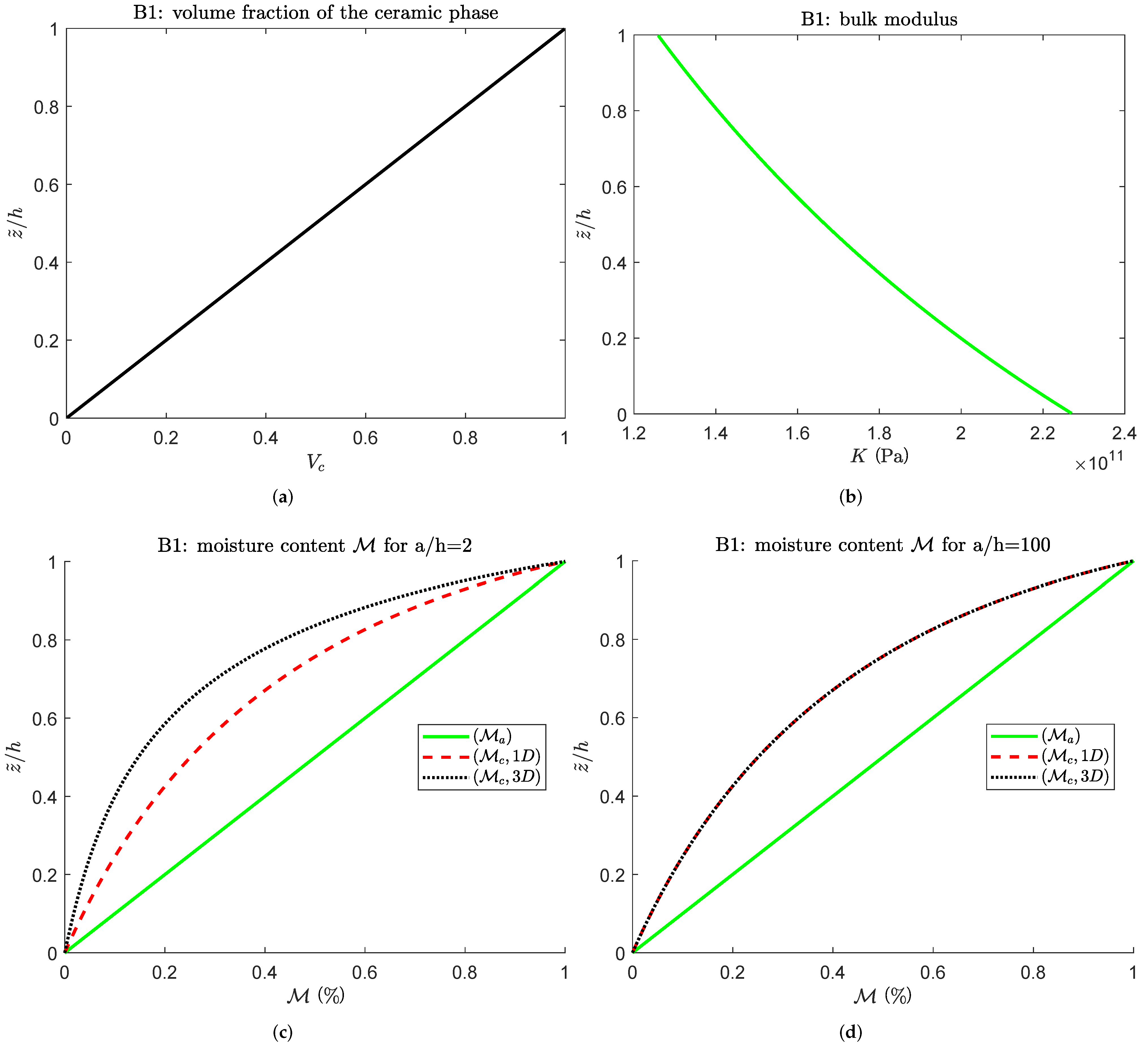The harmonic form of the moisture content has $m=n=1$ as half-wave numbers in $\alpha$ and $\beta$ directions, respectively. The elastic and hygroscopic properties of the metallic and ceramic phases are the same as those introduced at the beginning of this section. The FGM nature of the layer makes its mechanical properties evolve through the thickness direction; Figure 3a,b, respectively, shows how the volume fraction $V_c$ and the bulk modulus K evolve with respect to non-dimensional thickness coordinate $\tilde{z}/h$. Note that K is not linear as $V_c$ due to Equation (85).

Table 5. First benchmark: square plate with a single FGM layer subject to an external moisture content applied to the top and bottom surfaces. The results of all the 3D models consider $N=3$ and $NL=300$.

$\mathit{a}/\mathit{h}$	2	4	10	50	100
$\mathcal{M}$ at $(\alpha =a/2,\beta =b/2;\tilde{z}=4h/5)[-]$
3D(${\mathcal{M}}_a$)	0.8000	0.8000	0.8000	0.8000	0.8000
3D(${\mathcal{M}}_c,1D$)	0.5595	0.5595	0.5595	0.5595	0.5595
3D(${\mathcal{M}}_c,3D$)	0.4351	0.5197	0.5525	0.5592	0.5594
v at $(\alpha =a/2,\beta =0;\tilde{z}=4h/5)$ [mm]
3D(${\mathcal{M}}_a$)	−2.094	−2.089	−2.087	−2.086	−2.086
3D(${\mathcal{M}}_c,1D$)	−1.454	−1.461	−1.462	−1.462	−1.462
3D(${\mathcal{M}}_c,3D$)	−1.148	−1.362	−1.445	−1.462	−1.462
w at $(\alpha =a/2,\beta =b/2;\tilde{z}=h/2)$ [mm]
3D(${\mathcal{M}}_a$)	1.226	2.661	6.791	34.07	68.16
3D(${\mathcal{M}}_c,1D$)	1.103	2.405	6.144	30.83	61.68
3D(${\mathcal{M}}_c,3D$)	1.008	2.336	6.113	30.83	61.67
${\sigma }_{zz}$ at $(\alpha =a/2,\beta =b/2;\tilde{z}=h/5)$ [kPa]
3D(${\mathcal{M}}_a$)	−5915	−982.6	−127.7	−4.879	−1.218
3D(${\mathcal{M}}_c,1D$)	−1197	44.77	26.65	1.217	0.3054
3D(${\mathcal{M}}_c,3D$)	515.5	173.0	30.09	1.222	0.3057
${\sigma }_{\alpha \alpha }$ at $(\alpha =a/2,\beta =b/2;\tilde{z}=h)$ [MPa]
3D(${\mathcal{M}}_a$)	−7.939	−34.86	−43.94	−45.68	−45.73
3D(${\mathcal{M}}_c,1D$)	−63.24	−3.08	−89.55	−90.74	−90.78
3D(${\mathcal{M}}_c,3D$)	−90.78	−90.95	−90.83	−90.79	−90.79
${\gamma }_{\beta z}$ at $(\alpha =a/2,\beta =0;\tilde{z}=h/3)$ [${10}^{-6}$]
3D(${\mathcal{M}}_a$)	−173.7	−57.29	−18.35	−3.489	−1.741
3D(${\mathcal{M}}_c,1D$)	−39.06	3.440	4.709	1.072	0.5379
3D(${\mathcal{M}}_c,3D$)	19.67	12.49	5.321	1.076	0.5384

and Figure 4 report an extract of the main results. The results in tabular form give the amplitude of some variables of the problem; they reflect the three different ways of evaluating the moisture content. 3D(${\mathcal{M}}_a$) implies the assumed linear moisture content profile; 3D(${\mathcal{M}}_c,1D$) relies on the 1D version of the Fick moisture diffusion equation; finally, 3D(${\mathcal{M}}_c,3D$) relies on a 3D solution of the moisture diffusion problem. The prefix 3D underlines that the elastic part of the solution is three-dimensional in all three models. Such an analysis allows grasping the differences between the three approaches. The 3D(${\mathcal{M}}_c,3D$) shell model considers both the mechanical/hygrometric properties evolution through z and the three-dimensional nature of the problem. As discussed in the previous section, it always delivers an accurate result. Table 5 underlines that the 3D(${\mathcal{M}}_c,1D$) model results get closer to those of the 3D(${\mathcal{M}}_c,3D$) model as the thickness decreases. It considers how the mechanical/hygrometric properties evolve through z but disregards the moisture diffusion through alpha and beta direction, which have a negligible weight in thin structures. The results of the 3D(${\mathcal{M}}_a$) model are always unreliable, as they are built on a moisture content profile that is far from the actual scenario in a layer embedding an FGM. Figure 3c,d further facilitates understanding these concepts; it compares the three moisture content profiles for a thick and a thin plate. In thick structures, the difference between the three profiles is very pronounced: the three-dimensionality of the problem and the mechanical/hygrometric properties variability in the thickness direction make the 3D profile differ from the linear assumption. Even the 1D profile differs from the linearity: the hygrometric properties vary through z, reflecting on the moisture content at different thickness coordinates. These concepts also apply to thin structures; however, the three-dimensionality of the problem is insignificant, and the 3D and 1D profiles coincide. 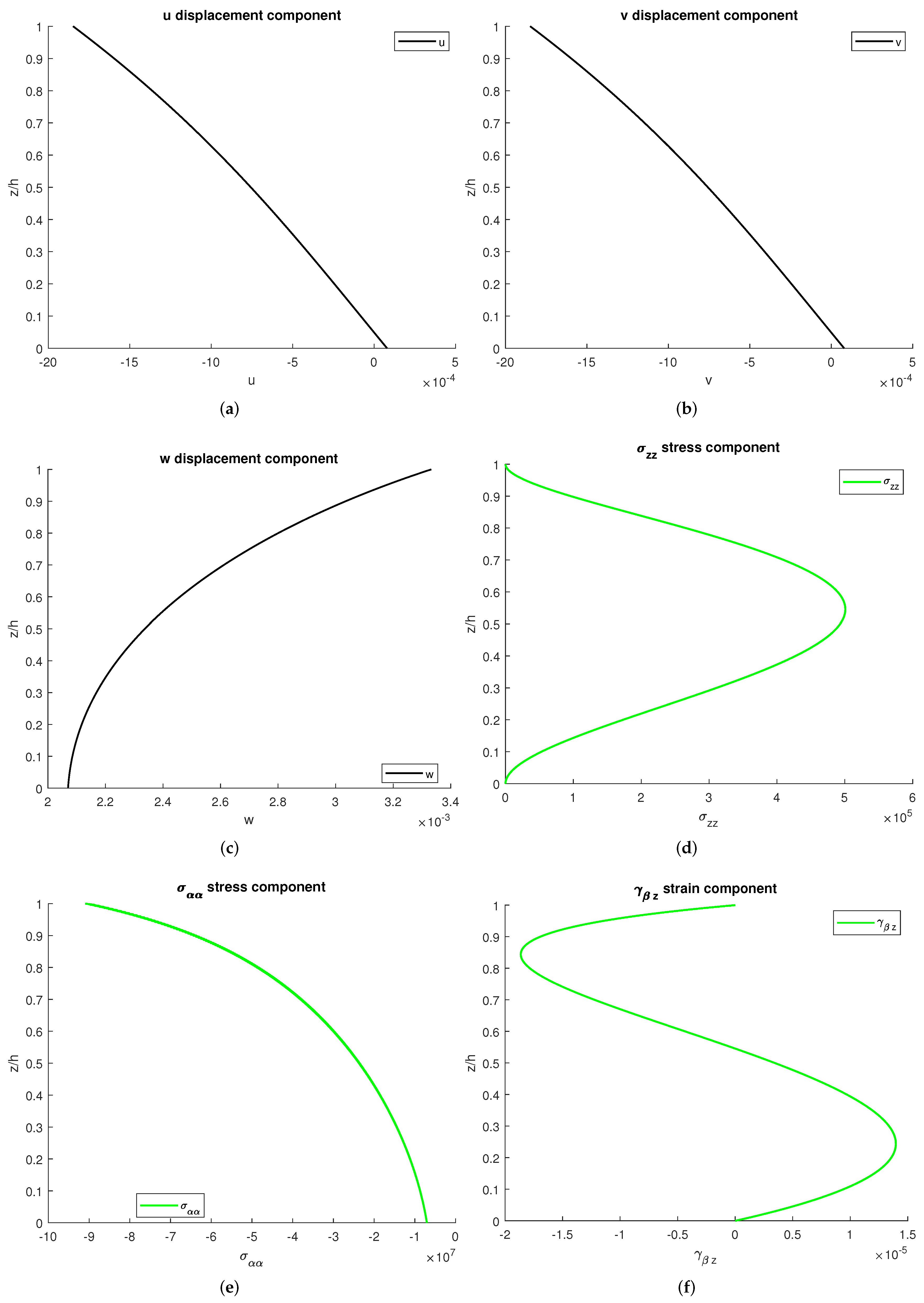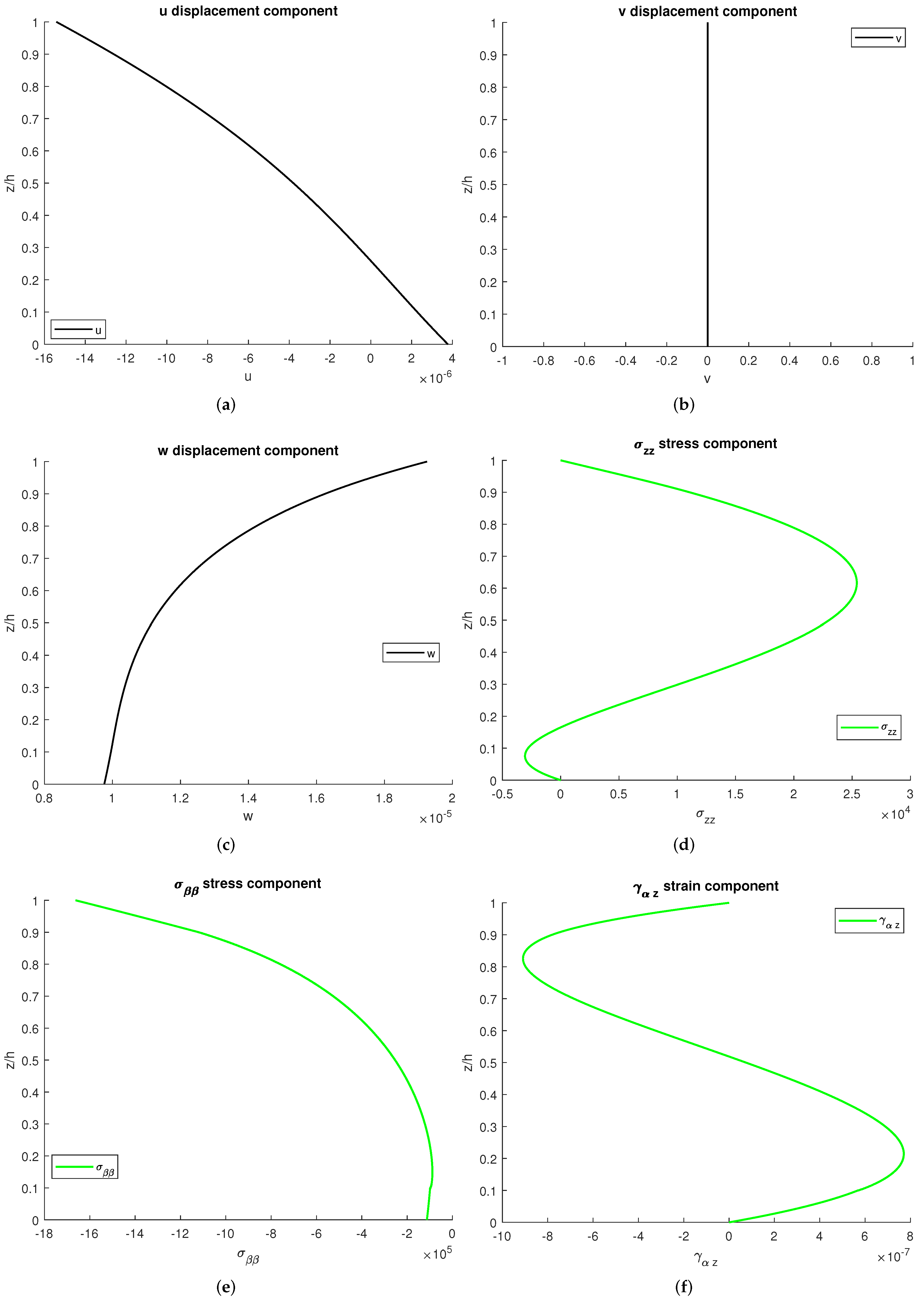Figure 4 shows the complete profile of the tree displacement components, two stresses, and a strain. Note that all the quantities evolve with continuity, which is essential as it demonstrates both the graded elastic/hygrometric properties and the correct introduction of the continuity conditions. The transverse stress ${\sigma }_{zz}$ and the transverse shear strain ${\gamma }_{\beta z}$ satisfy the external mechanical boundary conditions: it equals 0 at both the top and the bottom surfaces as no external load acts on them.

The second benchmark focuses on a closed cylinder, featuring a single FGM layer and simply-supported sides. The dimensions of the reference mid-surface, $a=2\pi R_{\alpha }$ and $b=30$ m, are a function of the radii of curvature of the shell, one of which is infinite: $R_{\alpha }=10$ m and $R_{\beta }=\infty$. Different thicknesses have been considered; the thickness ratio $R_{\alpha }/h$ is expressed with respect to $R_{\alpha }$ and ranges from 2 to 100 also in this second case study. The material volume fraction of the ceramic phase is a quadratic function of the thickness coordinate; the material law defined through Equation (83) consider $p=2$. Given that a single layer is considered, the cylinder is metallic in the inner surface and ceramic in the outer. The moisture content is imposed on the outer external surface, ${\mathcal{M}}_t=1.0\%$, and on the inner one, ${\mathcal{M}}_b=0.0\%$. The half wave numbers of both the harmonic forms are the same, $m=2$ and $n=1$. The elastic and hygroscopic properties of both the phases introduced previously also apply here. 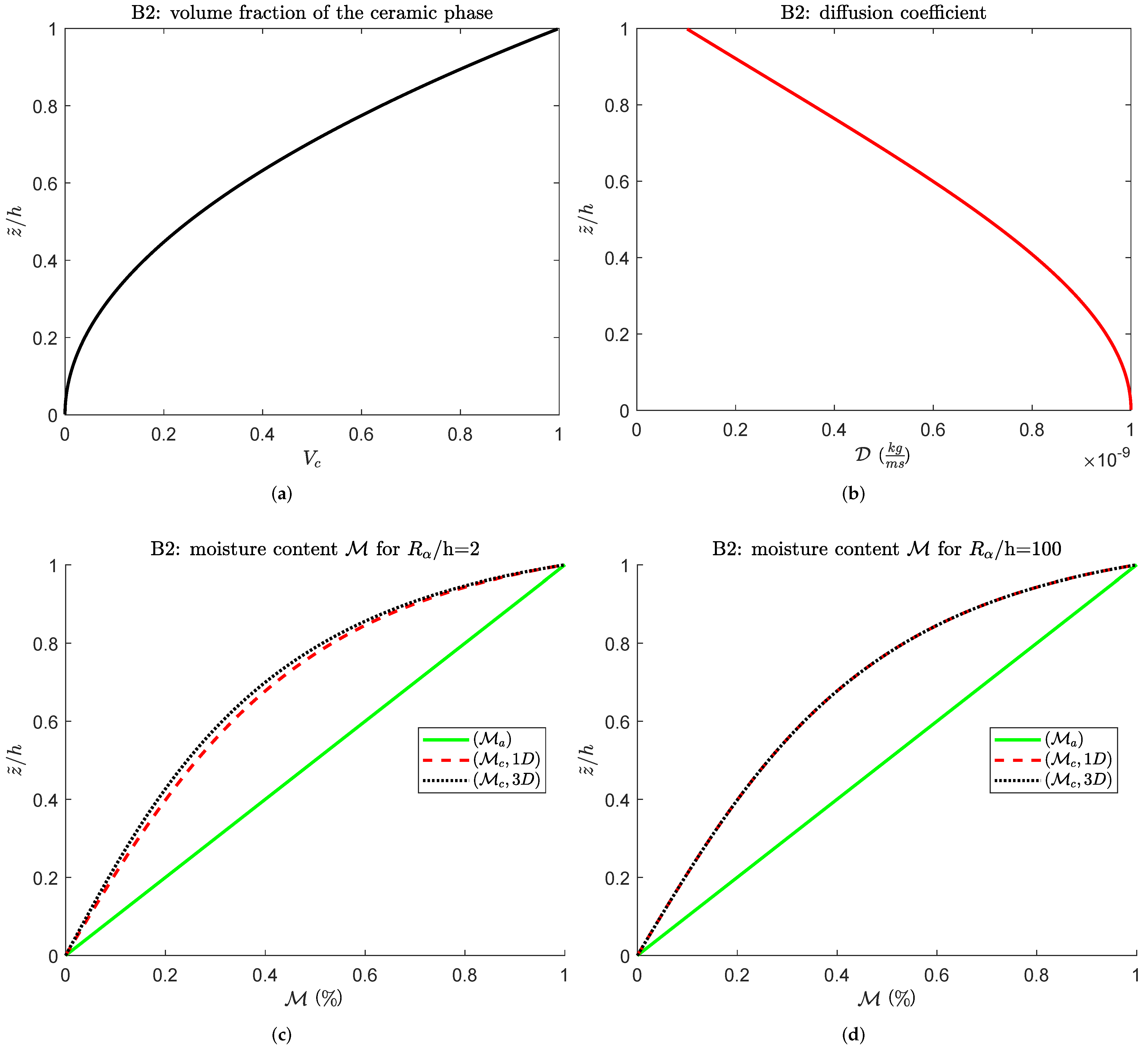Figure 5a,b, respectively, shows the volume fraction $V_c$ and moisture diffusion coefficient $\mathcal{D}$ vs. the non-dimensional thickness coordinate $\tilde{z}/h$. $V_c$ follows a power-law of order $p=2$, $\mathcal{D}$ follows Equation (85).

Table 6. Second benchmark: closed cylinder with a single FGM layer subject to an external moisture content applied to the top and bottom surfaces. The results of all the 3D models consider $N=3$ and $NL=300$.

${\mathit{R}}_{\mathit{\alpha }}/\mathit{h}$	2	4	10	50	100
$\mathcal{M}$ at $(\alpha =a/2,\beta =b/2;\tilde{z}=h/2)[-]$
3D(${\mathcal{M}}_a$)	0.5000	0.5000	0.5000	0.5000	0.5000
3D(${\mathcal{M}}_c,1D$)	0.2627	0.2627	0.2627	0.2627	0.2627
3D(${\mathcal{M}}_c,3D$)	0.2439	0.2577	0.2619	0.2626	0.2627
u at $(\alpha =0,\beta =b/2;\tilde{z}=h/3)$ [mm]
3D(${\mathcal{M}}_a$)	8.248	7.982	7.370	6.902	6.844
3D(${\mathcal{M}}_c,1D$)	5.538	5.125	4.582	4.210	4.161
3D(${\mathcal{M}}_c,3D$)	5.332	5.067	4.573	4.210	4.161
w at $(\alpha =a/2,\beta =b/2;\tilde{z}=h/2)$ [mm]
3D(${\mathcal{M}}_a$)	14.95	15.14	14.72	14.32	14.27
3D(${\mathcal{M}}_c,1D$)	9.600	9.488	9.056	8.714	8.667
3D(${\mathcal{M}}_c,3D$)	9.187	9.371	9.037	8.713	8.666
${\sigma }_{zz}$ at $(\alpha =a/2,\beta =b/2;\tilde{z}=2h/3)$ [MPa]
3D(${\mathcal{M}}_a$)	4.442	4.370	2.346	0.5349	0.2716
3D(${\mathcal{M}}_c,1D$)	7.308	5.035	2.383	0.5161	0.2605
3D(${\mathcal{M}}_c,3D$)	7.578	5.055	2.384	0.5161	0.2605
${\sigma }_{\beta \beta }$ at $(\alpha =a/2,\beta =b/2;\tilde{z}=h)$ [MPa]
3D(${\mathcal{M}}_a$)	37.63	−6.103	−36.31	−52.37	−54.33
3D(${\mathcal{M}}_c,1D$)	−53.79	−85.52	−106.3	−116.9	−118.2
3D(${\mathcal{M}}_c,3D$)	−60.83	−87.15	−106.5	−116.9	−118.2
${\gamma }_{\alpha \beta }$ at $(\alpha =0,\beta =0;\tilde{z}=0)$ $\left[{10}^{-6}\right]$
3D(${\mathcal{M}}_a$)	516.7	292.5	119.2	23.61	11.78
3D(${\mathcal{M}}_c,1D$)	390.8	209.0	82.62	16.12	8.025
3D(${\mathcal{M}}_c,3D$)	381.8	207.4	82.50	16.11	8.205

and Figure 6 summarize an extract of the main results. This second benchmark also reports three different sets of results: the elastic model is the same (prefix 3D), but the moisture content profile follows the different approaches. This leads to models 3D(${\mathcal{M}}_a$), in which the moisture content is a priori assumed, and 3D(${\mathcal{M}}_c,1D$)–3D(${\mathcal{M}}_c,3D$), in which the profile is calculated following a monodimensional or three-dimensional approach. This analysis allows highlighting the distinctions between the three methods. The last one is the only model in which no assumptions are made concerning the three-dimensionality of the problem as the moisture content amplitude derives from Fick’s law of diffusion. The results coming from 3D(${\mathcal{M}}_a$) are always wrong because the moisture content evaluation is inaccurate. The differences between 3D(${\mathcal{M}}_c,1D$) and 3D(${\mathcal{M}}_c,3D$) are less pronounced if compared with the previous benchmark and decrease with the thickness. The differences in the three moisture content profiles are shown in Figure 5c,d for two different cylinders: a thick and a thin one. The discrepancies between the calculated and assumed fields are really pronounced; the 1D and 3D computed profiles do not significantly differ, which is even more true as the thickness ratio increases. 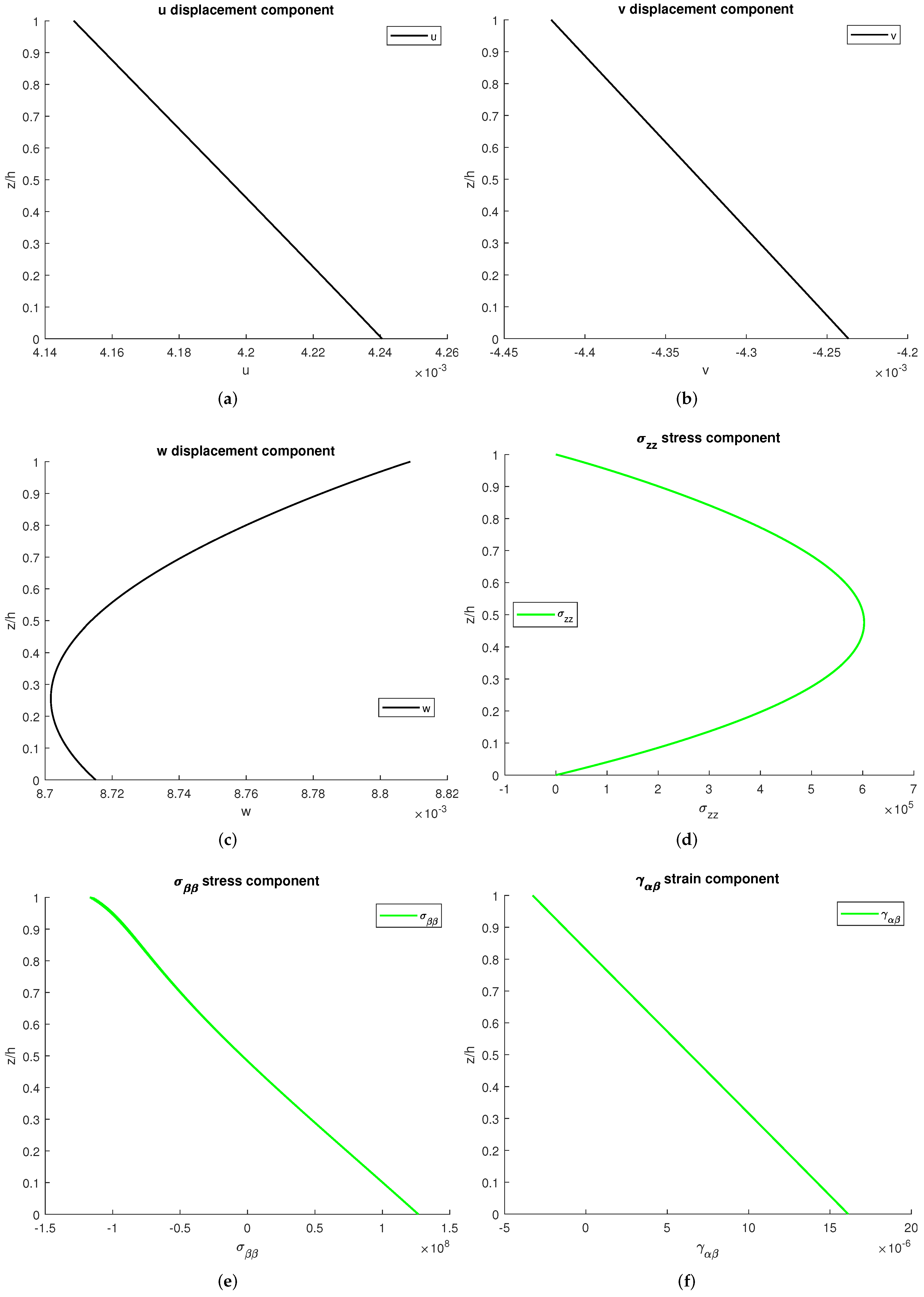Figure 6 shows the profiles of the tree displacement components: two stresses and a strain. There is continuity in all the plots: this qualifies the correct introduction of the continuity conditions and elastic/hygrometric properties grading. No external mechanical loads are applied, and this is coherent with the transverse stress values at the bottom and top surfaces, 0.

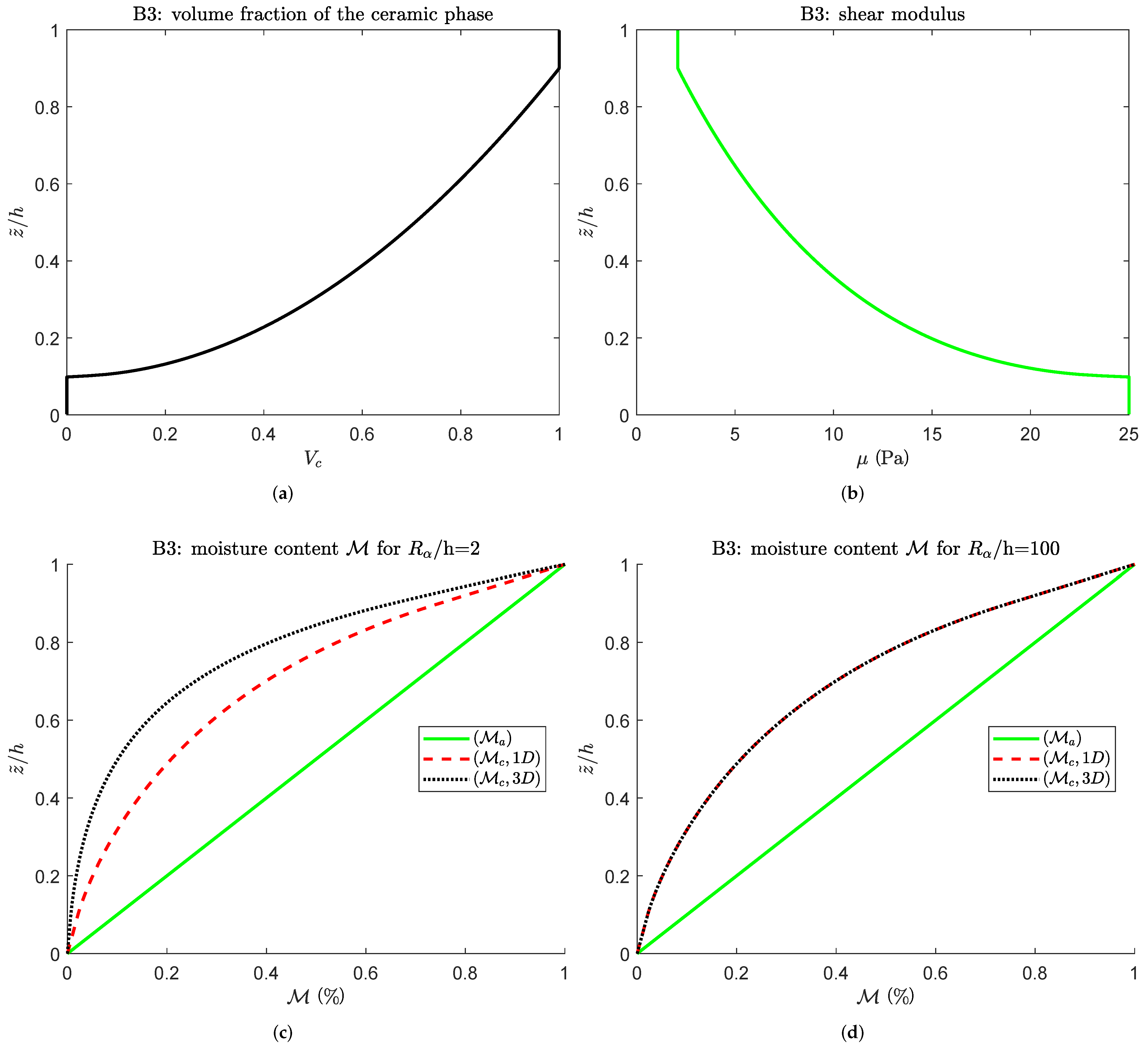
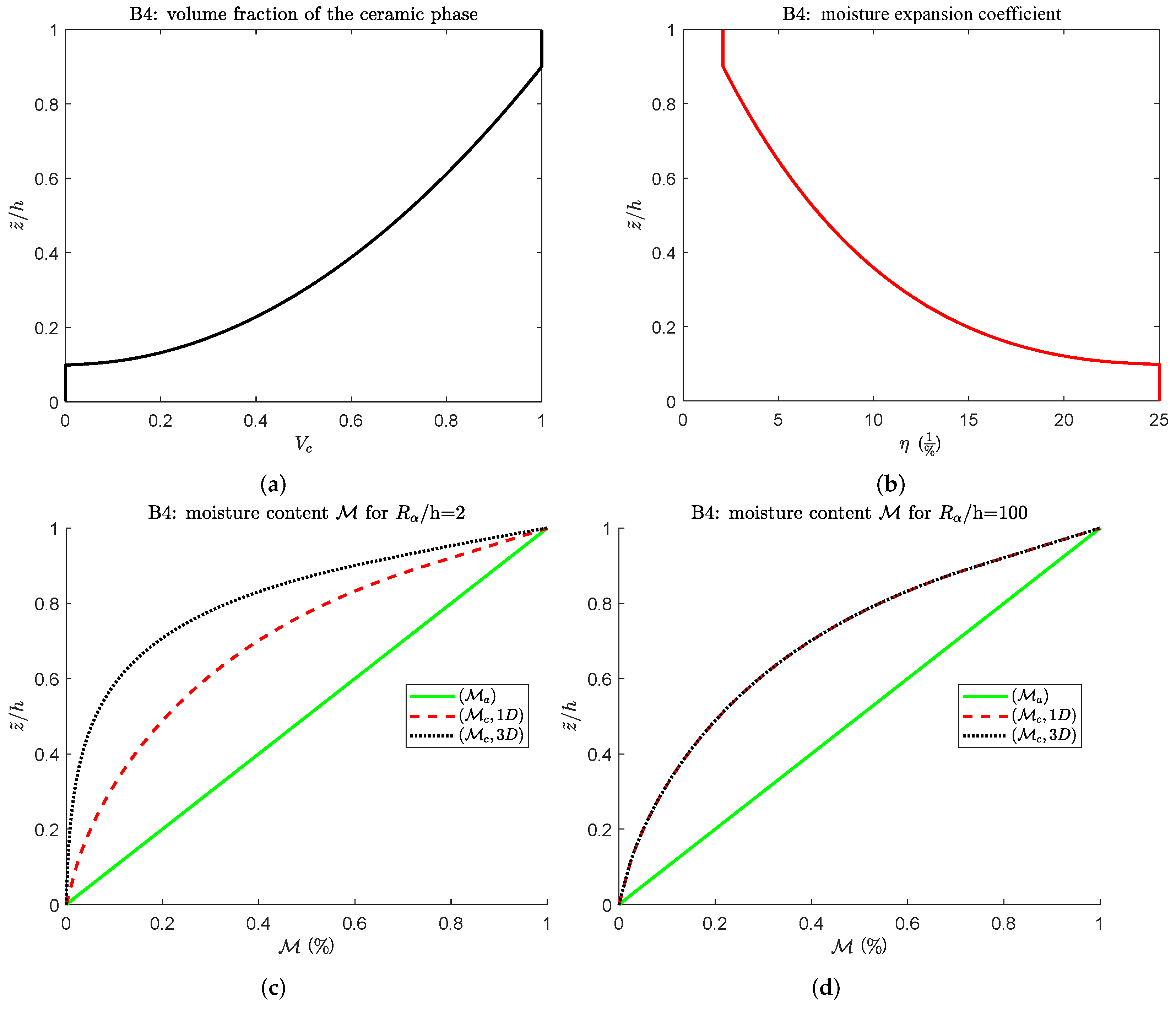
The third benchmark considers a cylindrical sandwich shell panel with an FGM core and simply-supported edges. The top and the bottom skin are in line with the FGM law: the top skin is ceramic as the top surface of the core is; at the same time, the bottom skin is metallic as the bottom surface of the core is. $p=0.5$ is the coefficient for the volume fraction law across the FGM core, which defines how the elastic and hygrometric properties evolve in the thickness direction. The elastic and hygroscopic properties of both the phases already introduced in the assessments also apply here. The radii of curvature are coherent with those proposed in the previous benchmark, $R_{\alpha }=10$ m and $R_{\beta }=\infty$. The dimension of the reference mid-surface in $\alpha$ direction is a function of the radius of curvature $R_{\alpha }$ and equals $a=\frac{\pi }{3}{R}_{\alpha }$; the dimension in the remaining direction $\beta$ is fixed and equals $b=30$. $m=2$ and $n=0$ have been chosen as half-wave numbers for the harmonic form of the moisture content imposed at the bottom and the top of the shell. The amplitude of the external fields discussed so far are as follows: the moisture content amplitude is ${\mathcal{M}}_t=1.0\%$ on the top and ${\mathcal{M}}_b=0.0\%$ on the bottom. This third case study also considers different thickness ratios to evaluate the effects of this parameter; as in the previous case, it is expressed with respect to $R_{\alpha }$ and ranges from 2 to 100. The volume fraction $V_c$ of the ceramic phase runs from 0 to 1 inside the core; it equals 0 inside the bottom skin as it is fully metallic, 1 inside the top coat as it is fully ceramic. 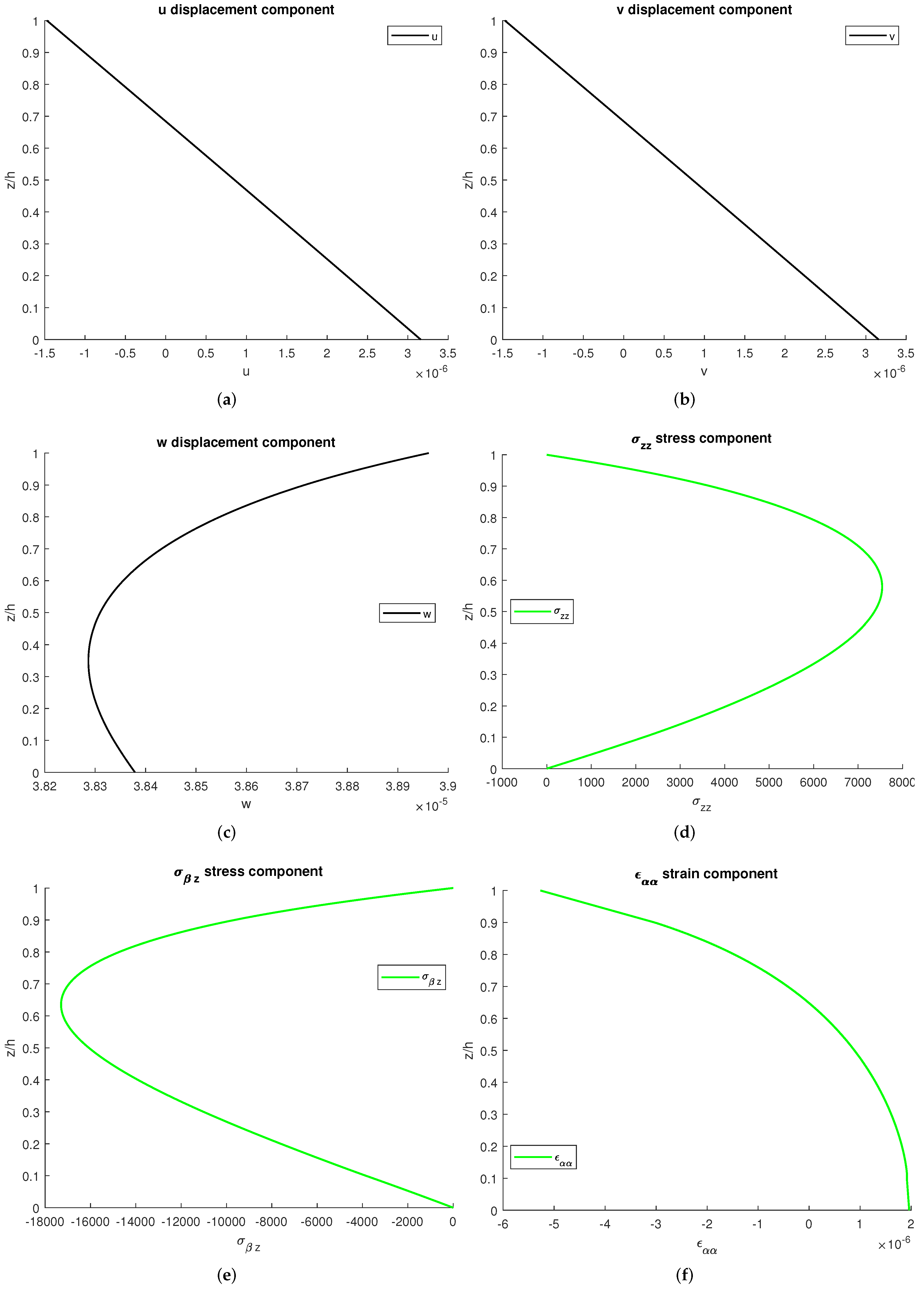This is visible in Figure 7a,b, showing the volume fraction and the shear modulus along with the thickness coordinate z; the shear modulus of the top skin coincides with that of the ceramic; the shear modulus of the bottom skin coincides with that of the metal. The amplitudes of some variables are reported for all the thickness ratios and at different thickness coordinates in

Table 7. Third benchmark: cylindrical sandwich shell panel with an FGM core subject to an external moisture content applied to the top and bottom surfaces. The results of all the 3D models consider $N=3$ and $NL=300$.

${\mathit{R}}_{\mathit{\alpha }}/\mathit{h}$	2	4	10	50	100
$\mathcal{M}$ at $(\alpha =a/2,\beta =b/2;\tilde{z}=h/2)[-]$
3D(${\mathcal{M}}_a$)	0.5000	0.5000	0.5000	0.5000	0.5000
3D(${\mathcal{M}}_c,1D$)	0.2087	0.2087	0.2087	0.2087	0.2087
3D(${\mathcal{M}}_c,3D$)	0.1014	0.1672	0.2008	0.2083	0.2086
u at $(\alpha =a/2,\beta =0;\tilde{z}=3h/4)$ [${10}^{-3}$ mm]
3D(${\mathcal{M}}_a$)	−16.26	−15.23	−11.79	11.86	41.40
3D(${\mathcal{M}}_c,1D$)	−10.53	−9.736	−6.559	15.20	42.34
3D(${\mathcal{M}}_c,3D$)	−7.942	−8.844	−6.416	15.20	42.34
w at $(\alpha =a/2,\beta =b/2;\tilde{z}=h/2)$ [${10}^{-5}$ mm]
3D(${\mathcal{M}}_a$)	0.5350	1.184	3.310	17.49	35.22
3D(${\mathcal{M}}_c,1D$)	0.5000	1.152	3.125	16.16	32.44
3D(${\mathcal{M}}_c,3D$)	0.4660	1.116	3.102	16.16	32.44
${\sigma }_{zz}$ at $(\alpha =a/2,\beta =b/2;\tilde{z}=h/4)$ [kPa]
3D(${\mathcal{M}}_a$)	−108.2	−7.415	0.3735	0.2473	0.1354
3D(${\mathcal{M}}_c,1D$)	0.6797	5.001	−1.110	−0.5867	−0.3135
3D(${\mathcal{M}}_c,3D$)	30.91	6.099	−1.162	−0.5875	−0.3136
${\sigma }_{\beta \beta }$ at $(\alpha =0,\beta =0;\tilde{z}=0)$ [kPa]
3D(${\mathcal{M}}_a$)	298.9	142.1	87.89	81.26	81.57
3D(${\mathcal{M}}_c,1D$)	−3.571	−92.06	−116.7	−116.9	−116.3
3D(${\mathcal{M}}_c,3D$)	−77.09	−112.7	−120.0	−117.0	−116.3
${\gamma }_{\alpha z}$ at $(\alpha =a/2,\beta =0;\tilde{z}=h/3)$ $\left[{10}^{-8}\right]$
3D(${\mathcal{M}}_a$)	−191.6	−51.36	−11.08	−1.956	−0.9857
3D(${\mathcal{M}}_c,1D$)	0.9706	46.64	26.65	5.584	2.790
3D(${\mathcal{M}}_c,3D$)	81.83	61.98	27.77	5.593	2.791

; Figure 8 explores six variables and shows their trend through z. The Figures rely on the 3D calculated moisture content profile; the table also reports the results obtained through ${\mathcal{M}}_a$ and ${\mathcal{M}}_c,1D$. The differences between the three models can be already seen at the moisture content level and directly reflect the mechanical quantities. Figure 7c,d compares the three moisture content profiles for a thick and a thin cylindrical shell panel and confirms that the differences are sharp not only at a specific thickness coordinate, but throughout all the thickness. The 3D(${\mathcal{M}}_c,1D$) model results get closer to those of the 3D(${\mathcal{M}}_c,3D$) model as the thickness decreases, and this is clear from the results of Table 7. Figure 8 gives the profile of the tree displacement components, two stresses, and a strain. As in the previous cases, all the quantities evolve with continuity: the mechanical properties are introduced into the model with continuity. The transverse stress ${\sigma }_{zz}$ satisfies the external mechanical boundary conditions: it equals 0 at both the top and the bottom surfaces as no external load acts on them.

The fourth and last benchmark proposes a sandwich spherical shell panel, which embeds an FGM core and features simply supported edges. The lamination scheme is analogous to that discussed in the third benchmark: the bottom skin is metallic, and the top ceramic. Then, the volume fraction of the ceramic phase evolves inside the core through the thickness direction following an exponential law with $p=0.5$ as chosen coefficients. The hygrometric and elastic properties of the sandwich skin are the same proposed in the previous benchmark and assessments for the metallic and ceramic phases, respectively; those of the core follow the volume fraction law. The exponential trend of the volume fraction $V_c$ vs. the non-dimensional thickness coordinate $\tilde{z}/h$ can be seen in Figure 9a; for completeness, the evolution of the moisture expansion coefficient $\eta$ through the thickness direction is also given in Figure 10. The spherical shell panel is the only structure among those studied in which both the radii of curvature are non-infinite; furthermore, they take the same value, which equals $R_{\alpha }=R_{\beta }=10$ m. Furthermore, the dimensions of the reference mid-surface are the same in $\alpha$, and $\beta$ directions as both are a function of the radii of curvature; it holds $a=\frac{\pi }{3}{R}_{\alpha }$ and $b=\frac{\pi }{3}{R}_{\beta }$. Those dimensions are fixed; however, a wide range of thinner/thicker shells is considered by choosing different thickness ratios: $R_{\alpha }/h$ ranges from 2 to 100. The amplitude of the moisture content is imposed on the top and the bottom surfaces; it equals ${\mathcal{M}}_t=1.0\%$ and ${\mathcal{M}}_b=0.0\%$, respectively. As discussed, the external fields are required to have a harmonic form in order for the problem to be exactly solved; $m=2$ and $n=2$ are the half-wave numbers considered in this last case study.

Table 8. Fourth benchmark, sandwich spherical shell panel with an FGM core subject to an external moisture content applied to the top and bottom surfaces. The results of all the 3D models consider $N=3$ and $NL=300$.

${\mathit{R}}_{\mathit{\alpha }}/\mathit{h}$	2	4	10	50	100
$\mathcal{M}$ at $(\alpha =a/2,\beta =b/2;\tilde{z}=h/2)[-]$
3D(${\mathcal{M}}_a$)	0.5000	0.5000	0.5000	0.5000	0.5000
3D(${\mathcal{M}}_c,1D$)	0.2087	0.2087	0.2087	0.2087	0.2087
3D(${\mathcal{M}}_c,3D$)	0.0612	0.1376	0.1933	0.2080	0.2085
v at $(\alpha =a/2,\beta =0;\tilde{z}=h/3)$ [${10}^{-3}$ mm]
3D(${\mathcal{M}}_a$)	−3.894	−2.822	−1.076	1.741	1.182
3D(${\mathcal{M}}_c,1D$)	−1.004	−0.628	0.4564	1.626	1.003
3D(${\mathcal{M}}_c,3D$)	0.2033	−0.1980	0.5091	1.625	1.003
w at $(\alpha =a/2,\beta =b/2;\tilde{z}=h/2)$ [${10}^{-3}$ mm]
3D(${\mathcal{M}}_a$)	4.294	9.003	24.12	59.21	58.93
3D(${\mathcal{M}}_c,1D$)	3.366	7.349	18.73	38.36	36.02
3D(${\mathcal{M}}_c,3D$)	2.910	6.711	18.31	38.31	36.00
${\sigma }_{zz}$ at $(\alpha =a/2,\beta =b/2;\tilde{z}=h/3)$ [kPa]
3D(${\mathcal{M}}_a$)	−337.9	−31.28	−0.2497	6.395	4.422
3D(${\mathcal{M}}_c,1D$)	−32.33	35.10	10.25	5.996	3.714
3D(${\mathcal{M}}_c,3D$)	85.74	45.62	10.43	5.991	3.713
${\sigma }_{\beta z}$ at $(\alpha =a/2,\beta =0;\tilde{z}=2h/3)$ [kPa]
3D(${\mathcal{M}}_a$)	240.7	125.3	61.39	−8.396	−9.287
3D(${\mathcal{M}}_c,1D$)	83.57	25.04	7.627	−17.21	−12.08
3D(${\mathcal{M}}_c,3D$)	13.41	3.374	5.225	−17.22	−12.08
${ϵ}_{\alpha \alpha }$ at $(\alpha =a/2,\beta =b/2;\tilde{z}=h)$ [${10}^{-6}$]
3D(${\mathcal{M}}_a$)	0.5547	−0.8651	−1.008	−2.249	−3.381
3D(${\mathcal{M}}_c,1D$)	−1.988	−3.376	−3.732	−5.260	−6.114
3D(${\mathcal{M}}_c,3D$)	−3.912	−4.182	−3.909	−5.268	−6.116

and Figure 9 and Figure 10 summarize an extract of the main results. This fourth benchmark also reports three different sets of results: the elastic model is the same (prefix 3D), but the moisture content profile follows the different approaches. This analysis highlights the distinctions between the three methods. The 3D one is the only model in which no assumptions are made concerning the three-dimensionality of the problem as the moisture content amplitude derives from Fick’s law of diffusion. The results coming from 3D(${\mathcal{M}}_a$) are always wrong because the moisture content evaluation is inaccurate. Considerable differences are present between the calculated and assumed fields. The moisture content profiles of Figure 9c,d once again demonstrate that the 1D and 3D moisture fields get closer in thin structures; despite the thickness, they always differ from the assumed profile, which completely disregards the physics of the problem. This reflects on the results in terms of displacements, strains, and stresses: the differences are high, and 3D(${\mathcal{M}}_a$) does not provide a reasonable estimate. 3D(${\mathcal{M}}_c,1D$) provides acceptable results, but only when the shell is sufficiently thin. As in the previous cases, three displacement components, two stresses, and a strain are shown in their entirety along with the thickness direction. Figure 10 further qualifies the correct introduction of the continuity conditions, elastic/hygrometric properties grading, and mechanical boundary conditions. The transverse stresses ${\sigma }_{\beta z}$ and ${\sigma }_{zz}$ satisfy the external mechanical boundary conditions: they equal 0 at both the top and the bottom surfaces as no external load acts on them. All the quantities are continuous throughout the thickness; this qualifies the division into fictitious layers: they are thin enough to describe the mechanical properties evolution with continuity.

5. Conclusions

The authors proposed a closed-form 3D shell solution that handles the hygro-elastic stress analysis of plates, cylinders, cylindrical shells, and spherical shells while embedding Functionally Graded Material (FGM) layers. First, the author imposed the external moisture content on the top and the bottom surfaces. The moisture conditions act in steady state as an external load; calculating the moisture content profile is a prerequisite. The authors showed that three approaches might be used to determine the moisture content profile along the thickness direction and coupled them with a consolidated elastic solution. The results demonstrated the importance of a correct moisture content profile evaluation in the thickness direction. The 3D Fick’s law of diffusion is the only way to obtain exact results when the structures embed FG layers; it is also necessary when the structures are sufficiently thick. On the other hand, the 1D Fick’s law of diffusion comes closer to it only when structures are thin; as a rule of thumb, the results of the two models are almost coinciding only from a thickness ratio of 50. The problem relies on a set of differential equations in the thickness direction. The authors demonstrated that the exponential matrix method is a reliable way to solve it, provided that the structures are divided into a sufficiently high number of mathematical layers. This layer-wise approach is critical to get a reliable description of the material properties grading; as a rule of thumb, 300 mathematical layers always deliver the correct results. This achievement is general and does not depend on the geometry, FGM law, and lamination sequence/scheme.

References

1. Zenkour, A.M. Hygro-thermo-mechanical effects on FGM plates resting on elastic foundations. Compos. Struct. 2010, 93, 234–238. [Google Scholar] [CrossRef]
2. Tabrez, S.; Mitra, M.; Gopalakrishnan, S. Modeling of degraded composite beam due to moisture absorption for wave based detection. CMES Comput. Model. Eng. Sci. 2007, 22, 77–90. [Google Scholar]
3. Swaminathan, K.; Sangeetha, D.M. Thermal analysis of FGM plates: A critical review of various modeling techniques and solution methods. Compos. Struct. 2017, 160, 43–60. [Google Scholar] [CrossRef]
4. Allahyarzadeh, M.; Aliofkhazraei, M.; Rouhaghdam, A.S.; Torabinejad, V. Gradient electrodeposition of Ni-Cu-W (alumina) nanocomposite coating. Mater. Des. 2016, 107, 74–81. [Google Scholar] [CrossRef]
5. Rezaiee-Pajand, M.; Sobhani, E.; Masoodi, A.R. Free vibration analysis of functionally graded hybrid matrix/fiber nanocomposite conical shells using multiscale method. Aerosp. Sci. Technol. 2020, 105, 105998. [Google Scholar] [CrossRef]
6. Sobhani, E.; Masoodi, A.R. Natural frequency responses of hybrid polymer/carbon fiber/FG-GNP nanocomposites paraboloidal and hyperboloidal shells based on multiscale approaches. Aerosp. Sci. Technol. 2021, 119, 107111. [Google Scholar] [CrossRef]
7. Sobhani, E.; Masoodi, A.R.; Ahmadi-Pari, A.R. Vibration of FG-CNT and FG-GNP sandwich composite coupled Conical-Cylindrical-Conical shell. Compos. Struct. 2021, 273, 114281. [Google Scholar] [CrossRef]
8. Rezaiee-Pajand, M.; Sobhani, E.; Masoodi, A.R. Semi-analytical vibrational analysis of functionally graded carbon nanotubes coupled conical-conical shells. Thin Walled Struct. 2021, 159, 107272. [Google Scholar] [CrossRef]
9. Sobhani, E.; Moradi-Dastjerdi, R.; Behdinan, K.; Masoodi, A.R.; Ahmadi-Pari, A.R. Multifunctional trace of various reinforcements on vibrations of three-phase nanocomposite combined hemispherical-cylindrical shells. Compos. Struct. 2022, 279, 114798. [Google Scholar] [CrossRef]
10. Rezaiee-Pajand, M.; Masoodi, A.R.; Mokhtari, M. Static analysis of functionally graded non-prismatic sandwich beams. Adv. Comput. Des. 2018, 3, 165–190. [Google Scholar]
11. Rezaiee-Pajand, M.; Rajabzadeh-Safaei, N.; Masoodi, A.R. An efficient curved beam element for thermo-mechanical nonlinear analysis of functionally graded porous beams. Structures 2020, 28, 1035–1049. [Google Scholar] [CrossRef]
12. Rezaiee-Pajand, M.; Masoodi, A.R.; Arabi, E. Geometrically nonlinear analysis of FG doubly-curved and hyperbolical shells via laminated by new element. Steel Compos. Struct. 2018, 28, 389–401. [Google Scholar]
13. Rezaiee-Pajand, M.; Arabi, E.; Masoodi, A.R. Nonlinear analysis of FG-sandwich plates and shells. Aerosp. Sci. Technol. 2019, 87, 178–189. [Google Scholar] [CrossRef]
14. Rezaiee-Pajand, M.; Masoodi, A.R. Analyzing FG shells with large deformations and finite rotations. World J. Eng. 2019, 5, 636–647. [Google Scholar] [CrossRef]
15. Das, N.C.; Das, S.N.; Das, B. Eigenvalue approach to thermoelasticity. J. Therm. Stress. 1983, 6, 35–43. [Google Scholar] [CrossRef]
16. Altay, G.A.; Dokmeci, M.C. Fundamental variational equations of discontinuous thermopiezoelectric fields. Int. J. Eng. Sci. 1996, 34, 769–782. [Google Scholar] [CrossRef]
17. Altay, G.A.; Dokmeci, M.C. Some variational principles for linear coupled thermoelasticity. Int. J. Solids Struct. 1996, 33, 3937–3948. [Google Scholar] [CrossRef]
18. Kosnski, W.; Frischmuth, K. Thermomechanical coupled waves in a nonlinear medium. Wave Motion 2001, 34, 131–141. [Google Scholar] [CrossRef]
19. Altay, G.A.; Dokmeci, M.C. Coupled thermoelastic shell equations with second sound for high-frequency vibrations of temperature-dependent materials. Int. J. Solids Struct. 2001, 38, 2737–2768. [Google Scholar] [CrossRef]
20. Cannarozzi, A.A.; Ubertini, F. A mixed variational method for linear coupled thermoelastic analysis. Int. J. Solids Struct. 2001, 38, 717–739. [Google Scholar] [CrossRef]
21. Brischetto, S.; Torre, R. 3D shell model for the thermo-mechanical analysis of FGM structures via imposed and calculated temperature profiles. Aerosp. Sci. Technol. 2019, 85, 125–149. [Google Scholar] [CrossRef]
22. Soldatos, K.P.; Ye, J. Axisymmetric static and dynamic analysis of laminated hollow cylinders composed of monoclinic elastic layers. J. Sound Vib. 1995, 184, 245–259. [Google Scholar] [CrossRef]
23. Messina, A. Three Dimensional Free Vibration Analysis of Cross-Ply Laminated Plates through 2D and Exact Models. In Proceedings of the 3rd International Conference on Integrity, Reliability and Failure, Porto, Portugal, 20–24 July 2009; pp. 20–24. [Google Scholar]
24. Fan, J.; Zhang, J. Analytical solutions for thick, doubly curved, laminated shells. J. Eng. Mech. 1992, 118, 1338–1356. [Google Scholar] [CrossRef]
25. Brischetto, S. Exact three-dimensional static analysis of single- and multi-layered plates and shells. Compos. Part B 2017, 119, 230–252. [Google Scholar] [CrossRef]
26. Brischetto, S. A closed-form 3D shell solution for multilayered structures subjected to different load combinations. Aerosp. Sci. Technol. 2017, 70, 29–46. [Google Scholar] [CrossRef]
27. Brischetto, S.; Torre, R. Convergence investigation for the exponential matrix and mathematical layers in the static analysis of multilayered composite structures. J. Compos. Sci. 2017, 1, 19. [Google Scholar] [CrossRef] [Green Version]
28. Brischetto, S.; Torre, R. A 3D layer-wise model for the correct imposition of transverse shear/normal load conditions in FGM shells. Int. J. Mech. Sci. 2018, 136, 50–66. [Google Scholar] [CrossRef]
29. Brischetto, S. A general exact elastic shell solution for bending analysis of functionally graded structures. Compos. Struct. 2017, 175, 70–85. [Google Scholar] [CrossRef]
30. Brischetto, S. Curvature approximation effects in the free vibration analysis of functionally graded shells. Int. J. Appl. Mech. 2016, 8, 1650079. [Google Scholar] [CrossRef]
31. Ozisik, M.N. Heat Conduction; John Wiley & Sons, Inc.: New York, NY, USA, 1993. [Google Scholar]
32. Povstenko, Y. Fractional Thermoelasticity; Springer: Berlin/Heidelberg, Germany, 2015. [Google Scholar]
33. Moon, P.; Spencer, D.E. Field Theory Handbook. Including Coordinate Systems, Differential Equations and Their Solutions; Springer: Berlin/Heidelberg, Germany, 1988. [Google Scholar]
34. Mikhailov, M.D.; Ozisik, M.N. Unified Analysis and Solutions of Heat and Mass Diffusion; Dover Publications Inc.: New York, NY, USA, 1984. [Google Scholar]
35. Tungikar, V.; Rao, B.K.M. Three dimensional exact solution of thermal stresses in rectangular composite laminates. Compos. Struct. 1994, 27, 419–439. [Google Scholar] [CrossRef]
36. Laoufi, I.; Ameur, M.; Zidi, M.; Abbes, A.B.E.; Boushala, A.A. Mechanical and hygrothermal behaviour of functionally graded plates using a hyperbolic shear deformation theory. Steel Compos. Struct. 2016, 20, 889–911. [Google Scholar] [CrossRef]
37. Inala, R. Influence of Hygrothermal Environment and FG Material on Natural Frequency and Parametric Instability of Plates. Mech. Adv. Compos. Struct. 2020, 7, 89–101. [Google Scholar]
38. Dai, T.; Dai, H.; Li, J.; He, Q. Hygrothermal mechanical behavior of a FG circular plate with variable thickness. Chin. J. Theor. Appl. Mech. 2019, 51, 512–523. [Google Scholar]
39. Zenkour, A.M.; Radwan, A.F. Bending and buckling analysis of FGM plates resting on elastic foundations in hygrothermal environment. Arch. Civ. Mech. Eng. 2020, 20, 234–238. [Google Scholar] [CrossRef]
40. Boukhelf, F. Hygro-thermo-mechanical bending analysis of FGM plates using a new HSDT. Smart Struct. Syst. 2018, 21, 75–97. [Google Scholar]
41. Zidi, M.; Tounisi, A.; Houari, M.S.A.; Bedia, E.A.; Beg, O.A. Bending analysis of FGM plates under hygro-thermo-mechanical loading using a four variable refined plate theory. Aerosp. Sci. Technol. 2014, 34, 512–523. [Google Scholar] [CrossRef]
42. Akbas, S.D. Hygro-thermal post-buckling analysis of a functionally graded beam. Coupled Syst. Mech. Int. J. 2019, 8, 459–471. [Google Scholar]
43. Chiba, R.; Sugano, Y. Transient hygrothermoelastic analysis of layered plates with one-dimensional temperature and moisture variations through the thickness. Compos. Struct. 2011, 93, 2260–2268. [Google Scholar] [CrossRef] [Green Version]
44. Gigliotti, M.; Jacquemin, F.; Molimard, J.; Vautrin, A. Modelling and experimental characterisation of hygrothermoelastic stress in polymer matrix composites. Macromol. Symp. 2007, 257, 199–210. [Google Scholar] [CrossRef]
45. Gigliotti, M.; Jacquemin, F.; Vautrin, A. Assessment of approximate models to evaluate transient and cyclical hygrothermoelastic stress in composite plates. Int. J. Solids Struct. 2007, 44, 733–759. [Google Scholar] [CrossRef]
46. Khalil, M.; Bakhiet, E.; El-Zoghby, A. Optimum design of laminated composites subjected to hygrothermal residual stresses. Proc. Inst. Mech. Eng. Part L J. Mater. Des. Appl. 2001, 215, 175–186. [Google Scholar] [CrossRef]
47. Kollár, L.P.; Patterson, J.M. Composite cylindrical segments subjected to hygrothermal and mechanical loads. Int. J. Solids Struct. 1993, 30, 2525–2545. [Google Scholar] [CrossRef]
48. Shen, H.-S. The effects of hygrothermal conditions on the postbuckling of shear deformable laminated cylindrical shells. Int. J. Solids Struct. 2001, 38, 6357–6380. [Google Scholar] [CrossRef]
49. Lee, S.Y.; Chou, C.J.; Jang, J.L.; Lin, J.S. Hygrothermal effects on the linear and nonlinear analysis of symmetric angle-ply laminated plates. Compos. Struct. 1992, 21, 41–48. [Google Scholar] [CrossRef]
50. Hufenbach, W.; Kroll, L. Stress analysis of notched anisotropic finite plates under mechanical and hygrothermal loads. Arch. Appl. Mech. 1999, 69, 145–159. [Google Scholar] [CrossRef]
51. Khoshbakht, M.; Lin, M.W.; Berman, J.B. Analysis of moisture-induced stresses in an FRP composites reinforced masonry structure. Finite Elem. Anal. Des. 2006, 42, 414–429. [Google Scholar] [CrossRef]
52. Kundu, C.K.; Han, J.-H. Vibration characteristics and snapping behaviour of hygro-thermo-elastic composite doubly curved shells. Compos. Struct. 2009, 91, 306–317. [Google Scholar] [CrossRef]
53. Kundu, C.K.; Han, J.-H. Nonlinear buckling analysis of hygrothermoelastic composite shell panels using finite element method. Compos. Part B 2009, 40, 313–328. [Google Scholar] [CrossRef]
54. Marques, S.P.C.; Creus, G.J. Geometrically nonlinear finite element analysis of viscoelastic composite materials under mechanical and hygrothermal loads. Comput. Struct. 1994, 53, 449–456. [Google Scholar] [CrossRef]
55. Naidu, N.V.S.; Sinha, P.K. Nonlinear finite element analysis of laminated composite shells in hygrothermal environments. Compos. Struct. 2005, 69, 387–395. [Google Scholar] [CrossRef]
56. Patel, B.P.; Ganapathi, M.; Makhecha, D.P. Hygrothermal effects on the structural behaviour of thick composite laminates using higher-order theory. Compos. Struct. 2002, 56, 25–34. [Google Scholar] [CrossRef]
57. Sereir, Z.; Adda-Bedia, E.A.; Tounsi, A. Effect of temperature on the hygrothermal behaviour of unidirectional laminated plates with asymmetrical environmental conditions. Compos. Struct. 2006, 72, 383–392. [Google Scholar] [CrossRef]
58. Sereir, Z.; Tounsi, A.; Adda-Bedia, E.A. Effect of the cyclic environmental conditions on the hygrothermal behavior of the symmetric hybrid composites. Mech. Adv. Mater. Struct. 2006, 13, 237–248. [Google Scholar] [CrossRef]
59. Sereir, Z.; Adda-Bedia, E.A.; Boualem, N. The evolution of transverse stresses in hybrid composites under hygrothermal loading. Mater. Des. 2001, 32, 3120–3126. [Google Scholar] [CrossRef]
60. Ram, K.S.S.; Sinha, P.K. Hygrothermal effects on the bending characteristics of laminated composite plates. Comput. Struct. 1991, 40, 1009–1015. [Google Scholar] [CrossRef]
61. Ram, K.S.S.; Sinha, P.K. Hygrothermal bending of laminated composite plates with a cutout. Comput. Struct. 1992, 43, 1105–1115. [Google Scholar] [CrossRef]
62. Benkhedda, A.; Tounsi, A.; Adda-Bedia, E.A. Effect of temperature and humidity on transient hygrothermal stresses during moisture desorption in laminated composite plates. Compos. Struct. 2008, 82, 629–635. [Google Scholar] [CrossRef]
63. Lo, S.H.; Zhen, W.; Cheung, Y.K.; Wanji, C. Hygrothermal effects on multilayered composite plates using a refined higher order theory. Compos. Struct. 2010, 92, 633–646. [Google Scholar] [CrossRef]
64. Parhi, P.K.; Bhattacharyya, S.K.; Sinha, P.K. Hygrothermal effects on the dynamic behavior of multiple delaminated composite plates and shells. J. Sound Vib. 2001, 248, 195–214. [Google Scholar] [CrossRef]
65. Raja, S.; Sinha, P.K.; Prathap, G.; Dwarakanathan, D. Influence of active stiffening on dynamic behaviour of piezo-hygro-thermo-elastic composite plates and shells. J. Sound Vib. 2004, 278, 257–283. [Google Scholar] [CrossRef]
66. Ghosh, A. Hygrothermal effects on the initiation and propagation of damage in composite shells. Aircr. Eng. Aerosp. Technol. Int. J. 2008, 4, 386–399. [Google Scholar] [CrossRef]
67. Szekeres, A. Analogy between heat and moisture thermo-hygro-mechanical tailoring of composites by taking into account the second sound phenomenon. Comput. Struct. 2000, 76, 145–152. [Google Scholar] [CrossRef]
68. Tay, A.A.O.; Goh, K.Y. A Study of Delamination Growth in the Die-Attach Layer of Plastic IC Packages under Hygrothermal Loading During Solder Reflow. In Proceedings of the 49th Electronic Components and Technology Conference, San Diego, CA, USA, 1–4 June 1999; pp. 694–701. [Google Scholar]
69. Tay, A.A.O.; Goh, K.Y. A study of delamination growth in the die-attach layer of plastic IC packages under hygrothermal loading during solder reflow. IEEE Trans. Device Mater. Reliab. 2003, 3, 144–151. [Google Scholar] [CrossRef]
70. Leissa, A.W. Vibration of Shells; NASA SP-288: Washington, DC, USA, 1973. [Google Scholar]
71. Boyce, W.E.; DiPrima, R.C. Elementary Differential Equations and Boundary Value Problems; John Wiley & Sons Ltd.: New York, NY, USA, 2001. [Google Scholar]
72. Open Document. Systems of Differential Equations. Available online: http://www.math.utah.edu/gustafso/ (accessed on 30 May 2013).
73. Reddy, J.N.; Cheng, Z.-Q. Three-dimensional thermomechanical deformations of functionally graded rectangular plates. Eur. J. Mech.-A/Solids 2001, 20, 841–855. [Google Scholar] [CrossRef]
74. Cinefra, M.; Carrera, E.; Brischetto, S.; Belouettar, S. Thermo-mechanical analysis of functionally graded shells. J. Therm. Stress. 2010, 33, 942–963. [Google Scholar] [CrossRef]
Figure 1. Geometrical data and coordinate system for plates and cylinders. The figure also shows the stacking sequence used in Benchmarks 1 and 2.
Applsci 12 00512 g001
Figure 2. Geometrical data and coordinate system for cylindrical and spherical shell panels. The figure also shows the stacking sequence used in Benchmarks 3 and 4.
Applsci 12 00512 g002
Figure 3. First benchmark: one-layered FGM ( p = 1 ) square plate with an imposed moisture content on the top and bottom surfaces. The figures show the volume fraction of the ceramic phase, the bulk modulus, and the moisture content profiles for a thick and a thin structure through their thickness. (a) Volume fraction of the ceramic phase V c . (b) Bulk modulus K. (c) Moisture content profile of the a / h = 2 plate. (d) Moisture content profile of the a / h = 100 plate.
Applsci 12 00512 g003
Figure 4. First benchmark: one-layered FGM square plate with an imposed moisture content on the top and bottom surfaces. The results are calculated for a moderately thick ( a / h = 4 ) structure via the 3D( M c , 3 D ) model. (a) Amplitude of u displacement component. (b) Amplitude of v displacement component. (c) Amplitude of w displacement component. (d) Amplitude of σ z z stress component. (e) Amplitude of σ α α stress component. (f) Amplitude of γ β z strain component.
Applsci 12 00512 g004
Figure 5. Second benchmark: one-layered FGM ( p = 2 ) cylinder with an imposed moisture content on the top and bottom surfaces. The figures show the volume fraction of the ceramic phase, the diffusion coefficient, and the moisture content profiles for a thick and a thin structure through their thickness. (a) Volume fraction of the ceramic phase V c . (b) Diffusion coefficient D . (c) Moisture content profile of the R α / h = 2 cylinder. (d) Moisture content profile of the R α / h = 100 cylinder.
Applsci 12 00512 g005
Figure 6. Second benchmark: one-layered FGM closed cylinder with an imposed moisture content on the top and bottom surfaces. The results are calculated for a moderately thin ( R α / h = 5 ) structure via the 3D( M c , 3 D ) model. (a) Amplitude of u displacement component. (b) Amplitude of v displacement component. (c) Amplitude of w displacement component. (d) Amplitude of σ z z stress component. (e) Amplitude of σ β β stress component. (f) Amplitude of γ α β strain component.
Applsci 12 00512 g006
Figure 7. Third benchmark: cylindrical sandwich shell panel featuring an FGM ( p = 0.5 ) core with an imposed moisture content on the top and bottom surfaces. The figures show the volume fraction of the ceramic phase, the shear modulus, and the moisture content profiles for a thick and a thin structure through their thickness. (a) Volume fraction of the ceramic phase V c . (b) Shear modulus μ . (c) Moisture content profile of the R α / h = 2 shell. (d) Moisture content profile of the R α / h = 100 shell.
Applsci 12 00512 g007
Figure 8. Third benchmark: cylindrical sandwich shell panel featuring an FGM ( p = 0.5 ) core with an imposed moisture content on the top and bottom surfaces. The results are calculated for a thick ( R α / h = 4 ) structure via the 3D( M c , 3 D ) model. (a) Amplitude of u displacement component. (b) Amplitude of v displacement component. (c) Amplitude of w displacement component. (d) Amplitude of σ z z stress component. (e) Amplitude of σ β β stress component. (f) Amplitude of γ α z strain component.
Applsci 12 00512 g008
Figure 9. Fourth benchmark: spherical sandwich shell panel featuring a FGM ( p = 0.5 ) core with an imposed moisture content on the top and bottom surfaces. The figures show the volume fraction of the ceramic phase, the moisture expansion coefficient, and the moisture content profiles for a thick and a thin structure through their thickness. (a) Volume fraction of the ceramic phase V c . (b) Moisture expansion coefficient η . (c) Moisture content profile of the R α / h = 2 shell. (d) Moisture content profile of the R α / h = 100 shell.
Applsci 12 00512 g009
Figure 10. Fourth benchmark: spherical sandwich shell panel featuring a FGM ( p = 0.5 ) core with an imposed moisture content on the top and bottom surfaces. The results are calculated for a thin ( R α / h = 50 ) structure via the 3D( M c , 3 D ) model. (a) Amplitude of u displacement component. (b) Amplitude of v displacement component. (c) Amplitude of w displacement component. (d) Amplitude of σ z z stress component. (e) Amplitude of σ β z stress component. (f) Amplitude of ϵ α α strain component.
Applsci 12 00512 g010