GSV-NET: A Multi-Modal Deep Learning Network for 3D Point Cloud Classification

Abstract

Light Detection and Ranging (LiDAR), which applies light in the formation of a pulsed laser to estimate the distance between the LiDAR sensor and objects, is an effective remote sensing technology. Many applications use LiDAR including autonomous vehicles, robotics, and virtual and augmented reality (VR/AR). The 3D point cloud classification is now a hot research topic with the evolution of LiDAR technology. This research aims to provide a high performance and compatible real-world data method for 3D point cloud classification. More specifically, we introduce a novel framework for 3D point cloud classification, namely, GSV-NET, which uses Gaussian Supervector and enhancing region representation. GSV-NET extracts and combines both global and regional features of the 3D point cloud to further enhance the information of the point cloud features for the 3D point cloud classification. Firstly, we input the Gaussian Supervector description into a 3D wide-inception convolution neural network (CNN) structure to define the global feature. Secondly, we convert the regions of the 3D point cloud into color representation and capture region features with a 2D wide-inception network. These extracted features are inputs of a 1D CNN architecture. We evaluate the proposed framework on the point cloud dataset: ModelNet and the LiDAR dataset: Sydney. The ModelNet dataset was developed by Princeton University (New Jersey, United States), while the Sydney dataset was created by the University of Sydney (Sydney, Australia). Based on our numerical results, our framework achieves more accuracy than the state-of-the-art approaches.

1. Introduction

3D sensors, including various LiDAR types, 3D scanners, and RGB-D cameras, such as RealSense, Kinect, and Apple depth cameras, have become more affordable and available with the fast evolution of 3D acquisition technologies [1]. The 3D data collected by these sensors can give various types of scaling geometric shape information [2,3,4]. The 3D data have more information than 2D images and allow machines to understand their surrounding environment better. Therefore, they have various applications in many fields, including robotics, self-driving cars, medical treatment, and remote sensing [5]. Different formats, including point cloud, depth images, volumetric grids, and meshes, can represent 3D data. Point cloud representation is a popular format that keeps the native geometric description in 3D space.

Point clouds are not only obtained by LiDAR sensors, depth cameras, stereo cameras, etc., but are also enhanced by additional sensors, such as multispectral, thermal, or color information [6,7,8]. The 3D point cloud stores 3D coordinates (x, y, z) and adds properties such as intensity and reflection. Furthermore, RGB-D images can construct the point cloud, and every (x, y) coordinate will match with four properties (R, G, B, and depth).

Point cloud classification can be applied to scene understanding such as robotics and autonomous driving [9,10,11]. In addition, point cloud classification is an essential task for the autonomous driving car because it helps the self-driving car identify objects on the roads. Some studies introduce several machine learning-based methods for point cloud classification [12,13,14]. Deep learning approaches have dominated various recent research fields, such as speech recognition or computer vision. Deep learning cannot apply directly to point cloud due to their irregular structure. Several researchers propose various deep learning-based solutions for point cloud classification, based on the view, the voxel, the raw-point cloud, and the graph. However, these approaches suffer from one or both of the following weaknesses: (1) missing test results with the real-world data that take from the LiDAR sensor, (2) having insufficiently good performance. In this work, we introduce a novel approach to overcome these above limitations.

Most classification techniques in the 3D point cloud cannot catch both visual and structural data because they employ a singular modal (see reference [15]). As a result, the classification rate is not high. We can obtain the advantage of each feature description from various modal information to improve classification accuracy. Multi-modals have potential development in point cloud classification. However, creating effective multi-modal is a challenging task. In this paper, we propose a novel framework GSV-NET, that employs both the point cloud and view-based model. GSV-NET captures both the global and the regional point cloud features with Gaussian Supervector (GSV) and the enhancing region representation (ERR). The complement of these features enriches the point cloud description and boosts the classification rate. Furthermore, combining Gaussian Supervector and enhancing region representation helps create an effective multi-modal. Figure 1 shows the structures of the proposed framework.

In this paper, our contributions are as follows:

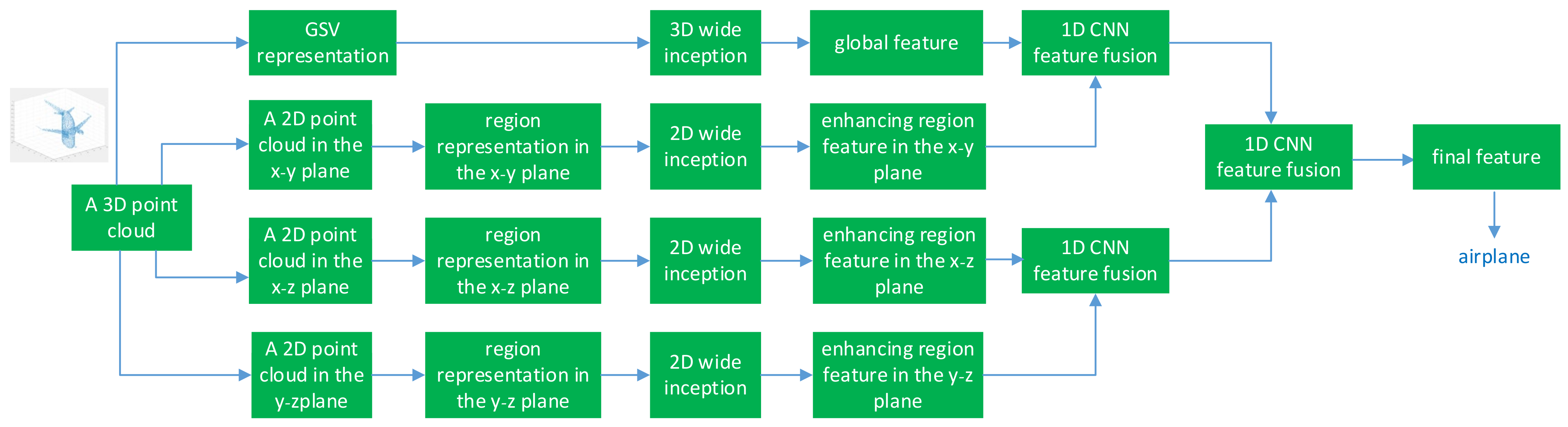
• We present a novel approach to extract the global point cloud feature using GSV representation and the 3D wide-inception architecture.
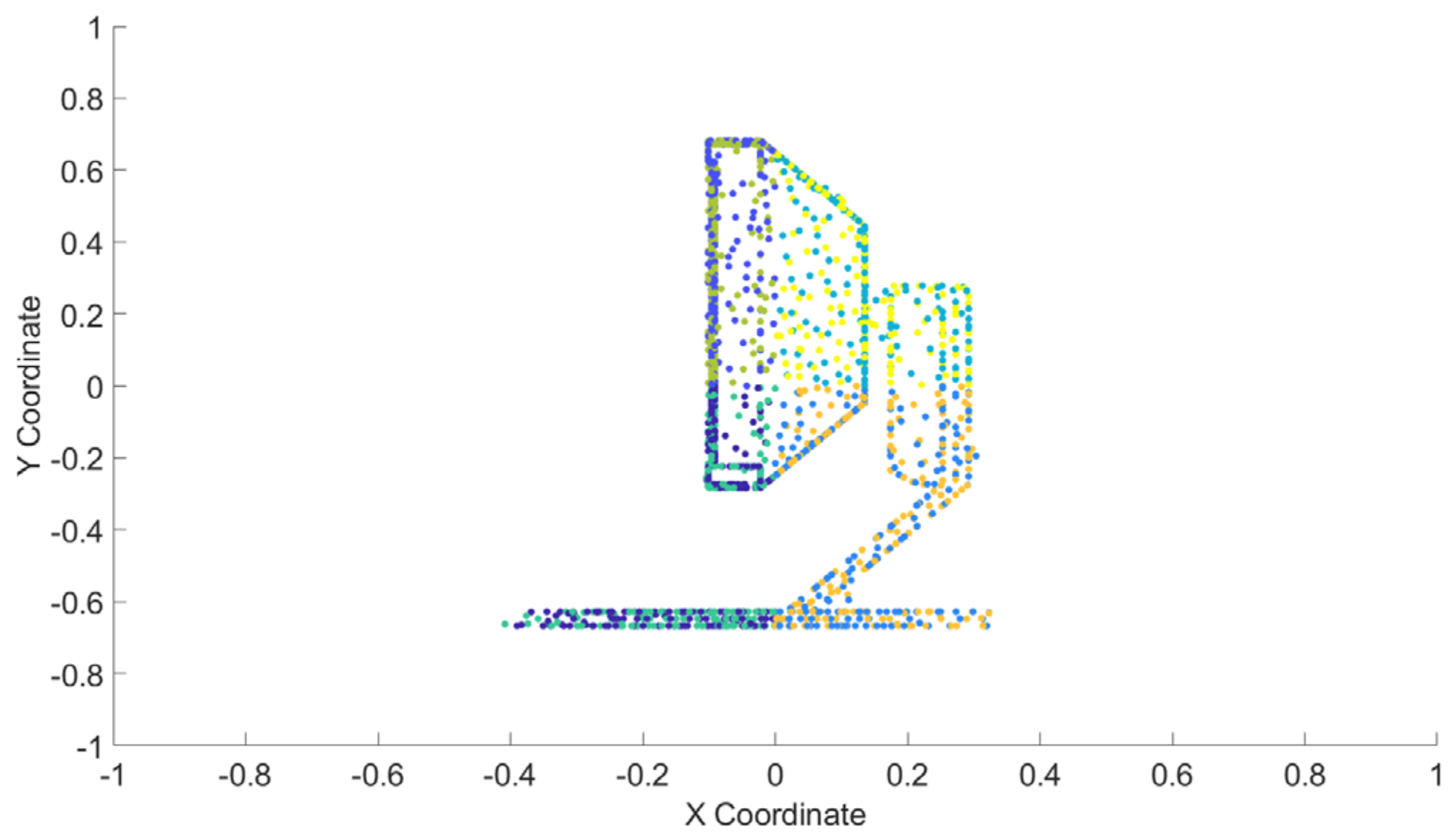
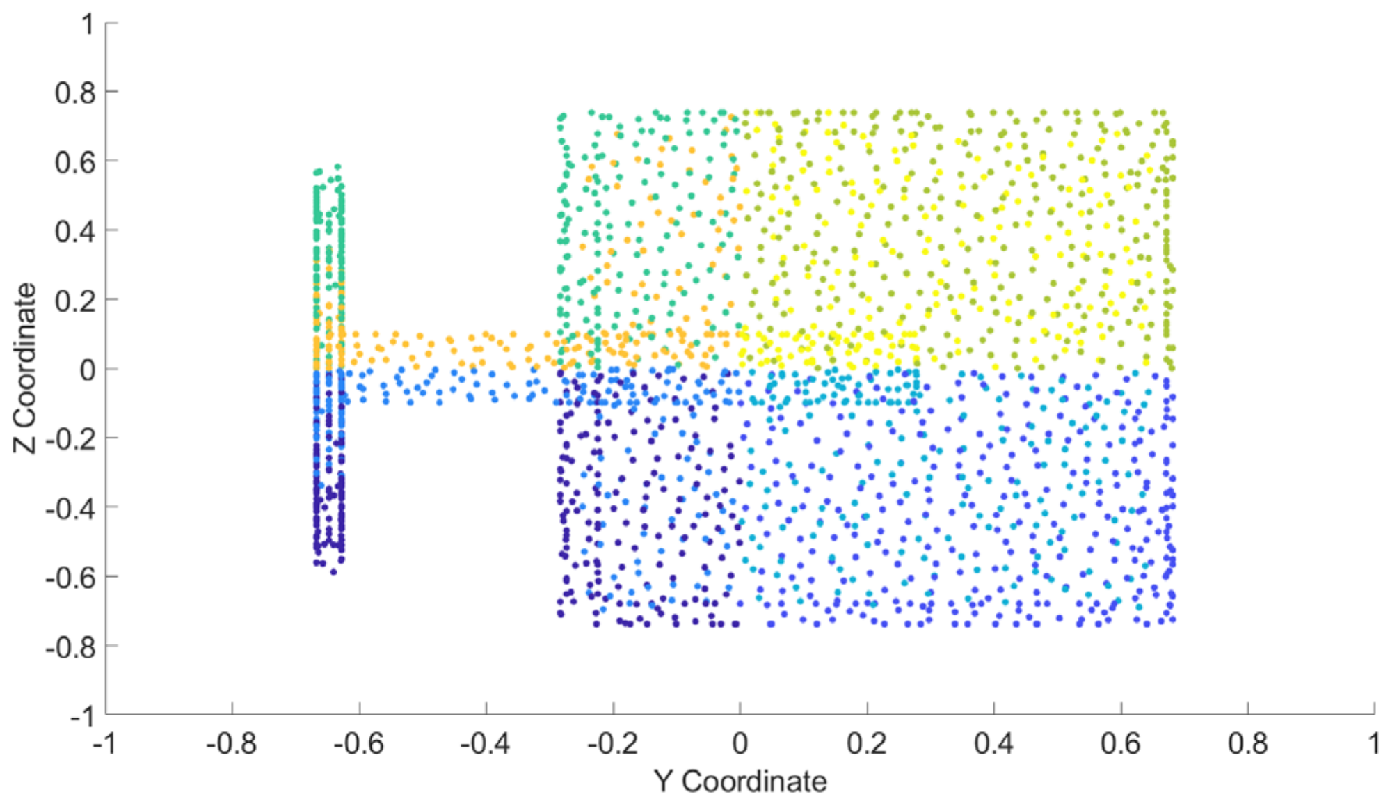
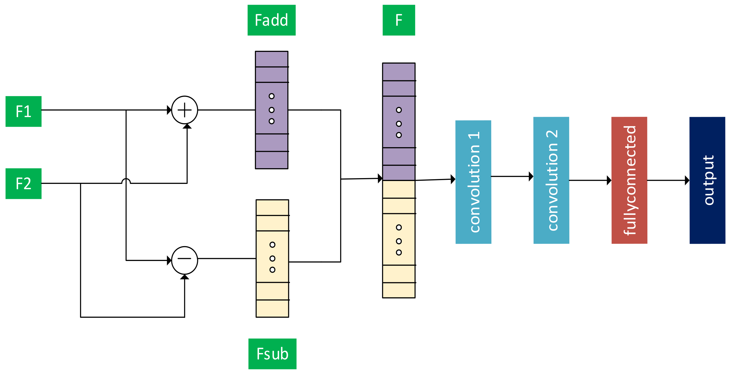
• After converting 3D point cloud regions into color representation, a 2D wide-inception network is employed to extract the regional feature of the 3D point cloud. In addition, we present the 1D convolution neural network (CNN) structure that fuses the extracted global and regional features. The GSV and ERR are novel to the best knowledge of the authors.
• Based on our numerical outcomes on challenging databases, the proposed approach is more accurate and efficient than the well-known methods.

The paper structure is as follows. We analyze the related works in Section 2, then define the proposed approach in Section 3. Section 4 shows the appropriate numerical environments, numerical outcomes, and analysis. Lastly, Section 5 represents achieving remarks.

2. Related Work

Recently, deep learning approaches have been the hotspot in 3D classification. CNN is designed for 2D images, and it cannot work directly with point cloud input due to its unordered and unstructured properties. The point cloud classification is based on four main approaches: voxel, multi-view, graph, and raw point cloud (see references [2,6,16]).

• Volumetric-based methods: These methods transform a point cloud into voxel and then use a 3D CNN to solve the shape-classification problem with the volumetric representation. Wu et al. [17] introduce a method: the deep belief network 3D ShapeNets, described by the distribution of the binary values on voxel grids for learning the distribution of points from different 3D objects. Maturana et al. [18] propose a volumetric occupation network (VoxNet) to obtain robust 3D shape classification. Although having promising results, these methods can not apply to big 3D data because the memory and the computation time increase cubically with voxel size. To handle the drawbacks, several authors propose a compact and hierarchical structure to reduce the memory and computational costs. Reference [19] introduces a 3D object recognition method, so-called OctNet, which implements 3D-CNN on the octants obtained by the 3D object surface. OctNet consumes less runtime and memory at higher points than a standard network based on dense input grids. OctNet divides a point cloud hierarchically using an octree structure, which describes the scenery with some octrees on a grid. Every voxel feature vector, cataloged by the uncomplicated arithmetic octree structure, is encoded efficiently utilizing a bit string description. Authors in [20] use 3D grids to describe the point cloud, represented by the 3D modified Fisher Vector, an input of CNN structure to produce the global description. Reference [21] offers a hybrid network PointGrid, which uses the grid description. PointGrid samples the points within each embedding volumetric grid-cell and uses 3D CNN to extract geometric details.
• Multiview-based methods: These approaches generate various 2D projections from the original 3D object, then obtain and fuse view-wise features for object recognition. The challenge is to integrate various view-wise features toward an overall description. Researchers in [22] firstly exploit the inter-relationships (view–view or region–region) across views by a leverage connection system, then integrate those views to obtain a discriminative 3D shape description. MHBN [23] adopts bilinear pooling to integrate local convolutional descriptors, then creates dense global features. MVCNN [24], only max-pooling multi-view descriptors toward global features, leads to information loss because max-pooling only holds the highest elements of a particular view.
• Raw point cloud-based methods: The initial point cloud is converted into voxel and views, respectively, in the two approaches mentioned above. Several researchers propose various methods to use the raw point cloud as input data without any transformation. Unlike the two approaches above, PointNet [25] employs a multilayer perceptron (MLP). This pioneering method leads a set of approaches that perform classification directly on the point cloud. PointNet converts the coordinates of the 3D point cloud to higher-dimensional descriptor space with the MLP. It also resolves the disorder obstacle and reduces the high-dimensional data by using max-pooling. Lastly, it employs the MLP to perform the recognition problem. PointNet++ [26] splits the point cloud toward various overlapping regions and uses PointNet to obtain the local descriptors in these regions. Local descriptors are continuously converted into global descriptors by repeated iterations to obtain the final descriptors. Motivated by the 2D SIFT [27], ref. [28] creates a PointSIFT module to describe data in many directions, and adjusts to the object proportion. An orientation-coding element is formed to represent eight essential orientations, and a multi-scale description is achieved by accumulating the multiple orientation coding elements. The PointSIFT network enhances presentation capacity by blending PointSIFT modules into several PointNet-based structures. PointCNN [29] first applies χ-transformation to resolve the obstacle of unordered and irregular structure in the point cloud, then uses the convolution approach for point cloud input.
• Graph-based methods: Graph Signal Processing (GSP) can handle unstructured or unordered data. GSP for preparing a 3D point cloud has been a popular field at current times, with many applications such as compression, painting, and data visualization [30,31,32,33]. GSP becomes essential because most data obtained can convert into a widespread graph. CNN introduces an effective architecture to exploit important patterns in regular structural data such as 2D images. Some approaches attempt to extend the concept of CNNs into widespread graphs, which are not straight because of the abnormal structure of these graphs. Defferrard et al. [34] define a recursive kernel of Chebyshev polynomials to introduce a quick localized convolution process, making it quickly learn while keeping sufficient complexity of deep learning. Bruna et al. [35] apply a graph convolution described in the graph spectral field. Graph-based methods implement a graph with an individual vertex for every point and edges within nearby points instead of converting point cloud toward voxels. A Graph-CNN structure in [36] uses the local architecture of the 3D point cloud data encoded in graphs to analyze 3D point cloud data. Graph-CNN requires neighbor data of every point at the best level for building a solid graph. In contrast, ref. [16] dismisses the uselessness by extracting a higher compact graph and making GSP on the Reeb graph.

In this work, the methods selected for comparison are based on data representation, including network structure. Those methods were fully representative of their subgroups.

Table 1. Principal approaches for point cloud classification.

			Methods
		Liang et al. [15]	Wang et al. [16]	Wu et al. [17]	Maturana et al. [18]	Riegler et al. [19]	BYizhak et al. [20]	Le et al. [21]	Yang et al. [22]	Yu et al. [23]	Su et al. [24]	Qi et al. [25]	Qi et al. [26]	Li et al. [29]	Defferrard et al. [34]	Bruna et al. [35]	Zhang et al. [36]	GSV-NET
Format	Voxelization			X	X	X
	Point cloud	X					X	X				X	X	X				X
	Views	X							X	X	X							X
	Graph		X												X	X	X
Dataset	Computer data	X	X	X	X	X	X	X	X	X	X	X	X	X	X	X	X	X
	Real-world				X	X	X											X
Architecture	MLP	X	X									X	X	X
	2D CNN	X							X	X	X							X
	3D CNN			X	X	X	X	X										X
	Graph CNN		X												X	X	X
Model	Single		X	X	X	X	X	X	X	X	X	X	X	X	X	X	X
	Multi-Modal	X																X

summarizes the principal methods for the point cloud classification based on input data format, dataset type, network architecture, and model type. A total of fifteen methods in the four main approaches, except Multimodal Information Fusion Network (MIFN) in reference [15] and GSV-NET, use a single model, leading to low performance in the point cloud classification. MIFN fuses three different models: the point cloud model, view model, and PANORAMA-view model, to obtain more-accurate classification results than those fifteen methods. However, there are two main drawbacks in MIFN: missing real-world datasets, and both the view model and PANORAMA-view model depend on the camera settings. Camera settings make MIFN hard to apply in real-life applications due to missing-view problems. Besides, 4 among 17 methods have testing results with real-world datasets, while the others use computer datasets. Computer data are different from the real-life data taken from the LiDAR sensor. Ignoring real-world data is a big drawback because real-world data ensure that the method works correctly with practical applications such as real-life self-driving systems.

GSV-NET performs best among 17 methods in the table due to some reasons. GSV-NET employs multi-modal to boost classification performance. Our framework fills the gap in the multi-modal approach. Unlike the first multi-modal, MIFN, GSV-NET effectively fuses model information and reduces the number of multi-modals. Specifically, GSV-NET has two models: point cloud model, and view model, compared with three models in MIFN: point cloud model, view model, and the PANORAMA-view model. In addition, GSV-NET handles two main drawbacks of MIFN: missing real-world datasets and camera-settings problems. In our proposed method, we first created three 2D point clouds from the original 3D point cloud based on the point locations and then convert them into three images, respectively. Hence, GSV-NET does not depend on camera settings. In contrast, MIFN and other view-based approaches place the camera surrounding the objects and capture the images. Moreover, the MIFN uses a total of 24 images for each 3D object (12 for the view model and 12 for the PANORAMA-view model), while GSV-NET uses only three.

3. Methodology

The GSV-NET was inspired by visual and structural complementary techniques (see reference [15]). We developed a new framework to handle the drawback of MIFN and MVCNN methods mentioned in the related work section. First of all, we choose the GSV representation and a novel 3D wide CNN instead of using a raw point cloud and MLP structure. The 3D CNN performs better than MLP in classification tasks (see reference [20]). Next, we replace the 2D view and panorama view in MIFN with the 2D color image containing region information. The region image provides more visual information than view and panorama view. As a result, GSV-NET reduces the number of images in MIFN from 24 to 3. Furthermore, we change the two-stage 2D CNN to a new 2D wide CNN. Lastly, we use 1D CNN to fuse the 1D vectors of the extracted features while MIFN employs features concatenation. The 1D CNN gives better performance compared to 2D CNN in the classification of the 1D signals (see reference [37]). GSV-NET employs two models, while MIFN uses three models. The numerical result verifies that our framework has the highest performance among methods.

Figure 1 shows the structure of the proposed framework. Firstly, we describe a point cloud as the input using the Gaussian Supervector representation, then put the GSV result in a 3D CNN architecture to extract the global point cloud feature. We employ a mixture of Gaussians with Gaussian centers on a uniform 3D m × m × m grid with optimal value m = 8 for the underlying density design, as mentioned in reference [20]. Secondly, we divide the original 3D point cloud into different regions based on the point locations. Next, we create three 2D point clouds (x-y, x-z, and y-z) and use 2D wide CNN to extract the enhancing region features of these 2D point clouds. Finally, a 1D CNN fuses the extracted features and creates the final point cloud feature. The following section will fully describe our framework: Gaussian Supervector representation in Section 3.1, enhancing region representation in Section 3.2, and 1D CNN feature fusion in Section 3.3.

3.1. Global Point Cloud Feature Extraction with Gaussian Supervector Representation and 3D Wide Inception

3.1.1. Gaussian Supervector Representation

First, we define the point cloud by the GSV representation. Let X = {$p_s\in R^3$, s = 1, …, S} be the set of 3D points (the point cloud), where S indicates the point number in the set. A D-dimensional Gaussian mixture for a single 3D point (or vector) $p_s$ is represented by the following form.

$$v\left(p_s\right)={\displaystyle \sum }_{k=1}^K{w}_k{v}_k\left(p_s;{\mu }_k,{\Sigma }_k\right),$$

(1)

where every $v_k, k=1, 2, \dots , K$ is the D-dimensional Gaussian density with the mean vector ${\mu }_k$, covariance matrix ${\Sigma }_k$, and weights $w_k>0$. Therefore, for every k,

$$v_k\left(p_s;{\mu }_k,{\Sigma }_k\right)=\frac{1}{{\left(2\pi \right)}^{\frac{D}{2}}\left(\sqrt{det{\Sigma }_k}\right)}{e}^{-\frac{1}{2}{\left(p_s-{\mu }_k\right)}^T{\Sigma }_k{}^{-1}\left(p_s-{\mu }_k\right)}.$$

(2)

In the case of a 3D point cloud (D = 3), Equation (2) can be re-written as:

$$v_k\left(p_s;{\mu }_k,{\Sigma }_k\right)=\frac{1}{{\left(2\pi \right)}^{\frac{3}{2}}\left(\sqrt{det{\Sigma }_k}\right)}{e}^{-\frac{1}{2}{\left(p_s-{\mu }_k\right)}^T{\Sigma }_k{}^{-1}\left(p_s-{\mu }_k\right)}$$

(3)

Bayes’ law is used to estimate the posterior probability distribution for every k value [38]. The soft assignment of point $p_s$ to the $k$-th Gaussian density is defined by:

$${\gamma }_k\left(p_s\right)=\frac{w_k{v}_k\left(p_s;{\mu }_k,{\Sigma }_k\right)}{{{\displaystyle \sum }}_{j=1}^K{w}_j{v}_j\left(p_s;{\mu }_j,{\Sigma }_j\right)}.$$

(4)

For every k = 1, 2, …, K, we define:

$$n_k={\displaystyle \sum }_{s=1}^S{\gamma }_k\left(p_s\right).$$

(5)

Gaussian Supervectors in [39] are used to handle the issue of natural view categorization. Using Equations (1)–(5), first determine the vector:

$$Z_k=\frac{{{\displaystyle \sum }}_{s=1}^S{\gamma }_k\left(p_s\right)\left(p_s-{\mu }_k\right)}{n_k}.$$

(6)

Then, for every k, calculate:

$$Z_k^{\prime }={\left(\frac{{\Sigma }_k}{n_k}\right)}^{-\frac{1}{2}} Z_k.$$

(7)

Finally, concatenate the vectors $Z_k^{\prime }$ to obtain the vector $Z_{KGSV}^{\prime }$. The resulting $Z_{KGSV}$ is normalized by the specimen size S [20]:

$$Z_{KGSVN}^{\prime }=\frac{1}{S} Z_{KGSV}^{\prime }.$$

(8)

Descriptions (particularly those concentrating on the maximum and minimum function) may improve the precision (see reference [38]). Hence, we apply the max and min functions on the $Z_{KGSVN}^{\prime }$ vector to create Gaussian Supervector representation $Z_{GSV}$ with the size at six by $K$. We have $K=m^3=8^3$ due to the optimal choice of m = 8, as explained in the Section 3.

3.1.2. 3D Wide-Inception Architecture

We reshape the GSV representation Z to the 4D matrix with the size of 8 × 8 × 8 × 6 and use it as the input for the 3D wide-inception CNN.

In the proposed 3D CNN network, we still adopt two kinds of 3D inception modules in reference [40]. The first applies the 3 × 3 × 3, and 1 × 1 × 1 kernel sizes, while the second splits the n × n × n filter into three filters with kernel sizes of n × 1 × 1, 1 × n × 1, and 1 × 1 × n, where n = 5 or 3. Besides, applying several convolution filters at the 1 × 1 × 1 size reduces the number of network parameters significantly due to a decrease in the dimension of the descriptor space.

We use a multi-scale block to choose the suitable kernel size. The kernel size holds a significant role in the training procedure and the model design because of valuable information extraction [41]. The bigger size of the kernel is suitable for global information, and the smaller size is better for catching the local data. The original inception network (see reference [42]) applies this concept and combines multiple convolutions with various kernel sizes.

The width, the depth, and the filter size are three significant factors in building a network structure (experimentally reported by He et al. [43]). Moreover, research on wide-residual networks [44] shows that a wide network design outperforms ResNets while keeping the ResNets shortcut connection [45]. Hence, this work offers a 3D wide-inception architecture to extract the global point cloud feature. In the proposed 3D CNN network, we stack two types of 3D inception modules together to expand the width of the network, thereby increasing the network performance and improving the flexibility of the network to features in various scales. Figure 2 shows the final architecture of the proposed 3D wide-inception network. The first four branches form the type-one module, while the type-two module consists of the last four branches, and each convolution layer has 64 filters.

3.2. Region Point Cloud Feature Extraction with 2D Wide Inception

3.2.1. Enhancing Region Representation

We divide the original 3D point cloud into different regions depending on points’ locations and convert it into the region’s representation. Each point has three coordinates (x, y, z), and each coordinate has a positive or negative sign, so we have a total of 2 ^ 3 = 8 different regions for the original 3D point cloud.

We have eight regions $R_1, R_2,\dots ,R_8$, as follows:

$$\begin{array}{c}{R}_1=\left\{p_s\in R^3 \mathrm{such} \mathrm{that} x_s>0, y_s>0, z_s\le 0\right\}.\\ R_2=\left\{p_s\in R^3 \mathrm{such} \mathrm{that} x_s>0, y_s\le 0, z_s\le 0\right\}.\\ R_3=\left\{p_s\in R^3 \mathrm{such} \mathrm{that} x_s\le 0, y_s>0, z_s\le 0\right\}.\\ R_4=\left\{p_s\in R^3 \mathrm{such} \mathrm{that} x_s\le 0, y_s\le 0, z_s\le 0\right\}.\\ R_5=\left\{p_s\in R^3 \mathrm{such} \mathrm{that} x_s>0, y_s>0, z_s>0\right\}.\\ R_6=\left\{p_s\in R^3 \mathrm{such} \mathrm{that} x_s>0, y_s\le 0, z_s>0\right\}.\\ R_7=\left\{p_s\in R^3 \mathrm{such} \mathrm{that} x_s\le 0, y_s>0, z_s>0\right\}.\\ R_8=\left\{p_s\in R^3 \mathrm{such} \mathrm{that} x_s\le 0, y_s\le 0, z_s>0\right\}.\end{array}$$

(9)

We create a colormap in Figure 3 based on eights regions, and the color values are chosen randomly. Figure 4 expresses the original 3D point cloud in eight different regions with eight corresponding colors. We use the color property because it helps 2D CNN to learn the region features easily. Next, we create three different 2D point clouds from three coordinates values of a 3D point cloud to better exploit the enhancing region features. The first 2D point cloud contains 2D points with the x–y coordinates of the original 3D point cloud. We can determine the regions $R_1, R_2,\dots ,R_8$ where the 2D points belong after removing the z coordinate. An enhancing region structure of the first 2D point cloud is encoded into a 2D color image with sizes 224 by 224 by 3 (see Figure 5). The encoding process is implemented by plotting the 2D point cloud with eight colors then exporting the result to an image. The color for each point in the 2D point cloud is decided by its region. For example, one point will have yellow if it belongs to the fifth region (see colormap in Figure 3). The process is the same for the other two 2D point clouds with the x–z coordinates, and the y–z coordinates, respectively. The 2D color image outputs are shown in Figure 6 and Figure 7.

3.2.2. 2D Wide-Inception Architecture

After creating the 2D color image of three 2D point clouds, we use three parallel 2D CNN to extract the region features. The three CNN branches have the same structure as one adopted from GoogLeNet architecture [46], also identified as IncpetionV1 design. The authors propose different variants such as InceptionV3 and InceptionV2 after the victory of InceptionV1. GoogLeNet structure applies various convolution layers within the same modules. Furthermore, it increases the network widely and deeply to take various images features. The most common GoogLeNet designs are the InceptionV3 and InceptionV1 structures. The InceptionV3 modules apply seven convolution layers, while six convolution layers are used in the InceptionV1 modules [47]. The InceptionV1 modules are used in this paper, as shown in Figure 8.

We use the long variant of the residual connection to increase the width of the original GoogLeNet structure. A network with a long-skip connection performs better overall and converges quicker (see reference [48]). The designs with a long-skip connection outperform the original network as it improves the reused features throughout the network.

In addition, long-skip connections support the network to learn both general features and detailed features of objects. The first feature comes from layers near the output, and the second feature is from layers close to input. Two different-sized layers are equally reshaped to perform a long-skip connection between them. Figure 9 displays the final 2D wide-inception architecture. We apply three skip convolution layers at the same kernel size of 1 × 1 to connect the input layers of inception modules: 3a, 4a, 5a, and an output layer of the inception module: 5b. Skip convolution layers one, two, and three have 64, 128, and 256 filters, respectively.

3.3. Feature Fusion with 1D CNN

We extract features from 2D CNN and 3D CNN at the fully connected layers, and each descriptor extracted is a 1D vector with the size at 1 × T (T is the number of the classes). The 1D CNN performs better compared to 2D CNN in dealing with 1D signals (see reference [37]). Therefore, we use a 1D CNN structure to fuse the extracted features, as shown in Figure 2. Given two inputs $F_1$ and $F_2$, each feature vector has the size at 1 × T. We apply the following addition and subtraction.

$$F_{add}=\frac{F_1+F_2}{2}.$$

(10)

$$F_{sub}=\frac{F_1-F_2}{2}.$$

(11)

Finally, we concatenate the vectors $F_{add}$ and $F_{sub}$ to form the final input vector F with a size of 1 × 2T. Figure 10 presents the structure of the fusion block. Both 1D convolution layers: one and two have the same kernel size at 1 × 3 with 16 and 32 filters, respectively.

4. Experiment

In this section, we evaluate the proposed framework GSV-NET on both computer datasets and real-world datasets. For each point cloud in the training dataset, our framework extracts its final feature, then assigns the corresponding “true” label from training labels. After finishing training, the framework obtains the final point cloud feature to predict the label for each point cloud in the testing dataset. We obtain the predicted labels and compare them with “true” labels of the testing dataset, then calculate the following metrics: the precision, the recall, the F1 score, and the accuracy. Based on the numerical result, we compare the performance of GSV-NET with other state-of-the-art methods. The following section will fully describe our experiment: datasets in Section 4.1, evaluation metrics in Section 4.2, implementation details in Section 4.3, the comparison on ModelNet40 dataset in Section 4.4, and the comparison on Sydney datasets in Section 4.5.

4.1. Datasets

The proposed method is estimated on the point cloud dataset: ModelNet40 [17] and LiDAR dataset: Sydney Urban Objects [49].

ModelNet40: ModelNet40 has 12,311 objects from 40 categories. The datasets are split into two parts: one with 2468 testing objects and one with 9841 training objects (see reference [17]).

Sydney Urban Objects: Deuge et al. (2013) [50] applied their segmentation methods on some sequences of Velodyne scans to create this dataset. It is split into four folds, and it includes 588 labeled point clouds in 14 classes such as pedestrians, vehicles, trees, signs, etc. This dataset is modeled by the sparse point clouds. This dataset shows variability in viewpoint, and it is not an ideal sensing situation with occlusions [51]. It would be a difficult task to identify models from this dataset.

4.2. Evaluation Metrics

We use an accuracy metric to evaluate the ModelNet dataset and the weighted F1 (see reference [52]) for the Sydney dataset. We measure the precision, the recall, and the F1 score for each class u in the dataset for the calculations of the weighted F1.

$$Precisio{n}_u=\frac{T{P}_u}{T{P}_u+F{P}_u},$$

(12)

$$Recal{l}_u=\frac{T{P}_u}{T{P}_u+F{N}_u},$$

(13)

$$\mathrm{F}{1}_u=2\times \frac{Precisio{n}_u\times Recal{l}_u}{Precisio{n}_u+Recal{l}_u},$$

(14)

$$W_u=\frac{N_u}{{{\displaystyle \sum }}_{v=0}^T{N}_v},$$

(15)

$$\mathrm{The} \mathrm{weighted} \mathrm{F}1={\displaystyle \sum }_{u=0}^T{W}_u\times \mathrm{F}{1}_u,$$

(16)

where $N_u$ is the number of models of class u; T is the number of categories; $T{N}_u$ is the true negative of category u; $T{P}_u$ is the true positive of category u; $F{N}_u$ is the false negative of category u; $F{P}_u$ is the false positive of category u.

4.3. Implementation Details

The original Sydney and ModelNet datasets can be obtained from the website in the Data Availability Statement. All experiments were performed on the i7 7700 PC, with memory of 32 GB, 1080TI GPU (11 GB memory), MATLAB (9.9 (R2020b), Natick, MA, USA). We employ the initial learning rate at 0.001 for 2D and 3D CNN while applying 0.0002 for 1D CNN. We divide the learning rate by half after every 20 epochs, the mini-batch at 32 for SGD, and the momentum at 0.9 for network training.

4.4. The Comparison on ModelNet40 Dataset

We test GSV-NET on the ModelNet40 dataset with different approaches on four main data representations (voxel, point, graph, and image).

Table 2. Comparison with various approaches on the point cloud dataset: ModelNet40.

Method	Data Format	ACC
VoxNet [18]	Voxelization	83%
3D ShapeNets [17]	Voxelization	77.32%
3D-A-Nets [53]	Voxelization	90.5%
EEM [54]	Point Cloud	90.5%
PointGCN [36]	Point Cloud	89.5
PointNet [25]	Point Cloud	89.2%
PointNet++ [26]	Point Cloud	90.7%
3DmFV+VoxNet [20]	Point Cloud	88.5%
3DmFV-Net [20]	Point Cloud	91.6%
MVCNN, metric,12× [24]	12 views	89.5%
MVCNN, 12× [24]	12 views	89.9%
MVCNN, metric,80× [24]	80 views	90.1%
MVCNN, 80× [24]	80 views	90.1%
TCN-MVCNN [55]	12 views	90.5%
Reeb graph convolution [16]	graph	89.9%
MIFN, PC+MV [15]	Point Cloud + 12 views	90.83%
MIFN, PC+MV+PV [15]	Point Cloud + 12 views + panorama-views	91.86%
GSV-NET	Point Cloud + 3 views	92.7%

shows the recognition outputs of all methods, and our proposed framework obtains the most excellent performance, with a classification rate of 92.7% for ModelNet40.

GSV-NET outperforms a pioneering approach, PointNet, using the natural point cloud. The symmetric max-pooling function is applied to obtain a global descriptor. However, PointNet does not capture the local structure because it does not examine the local dependency between points, leading to an accuracy rate of 89.2%. To handle the drawback of PointNet, PointNet++ splits the point cloud into different regions to obtain the local descriptor and increases the accuracy rate to 90.7%. Another method, PointGCN, obtains local descriptors by the kNN graph but neglects global connections among these local descriptors. It has classification results of 89.5%. The best performance method in the point cloud group is the 3DmFV method, having a precision of 91.6% (3DmFV-Net).

Although performing well, voxel-based methods consume high memory due to voxels’ sparsity, resulting in wasted calculations for convolution across the non-occupied areas. The memory usage also restricts the voxel presentation, commonly in the range of 32 to 64 cubes. Therefore, VoxNet, 3D-A-Nets, and 3DShapeNets produce low accuracy of 83%, 90.5%, and 77.32%, respectively. Multiview-based approaches (MVCNN) achieve a better result than voxel-based methods because they apply a well-known 2D CNN, resulting in high accuracy of 90.1%. Unlike the multi-view or voxel-based approach, the graph-based method fits the irregular data processing like 3D shape classification. The graph-based method takes advantage of the sparsity of the point cloud. However, a challenging and further study is to design efficient convolution, pooling modules for graph-based networks. There is still a gap between the Reeb graph and the multiview-based approach such as MVCNN. Hence, the Reeb graph gives a precision of 89.9%.

The 3D point cloud provides objects’ information suitable for classifying shapes with diverse scales, while the 2D image gives much texture data better for specifying shapes with indistinguishable appearances [56,57]. The merging of these two types of information is useful to improve the representation of the extracted features for classification purposes. MIFN merges the 3D information that comes from PointNet architecture and the 2D data that come from MVCNN. However, the MVCNN takes only the projection of the 3D models without the regional information. In contrast, GSV-NET captures not only global representation, but also regional representation. Moreover, GSV-NET uses 2D point locations and does not depend on a camera setting, while MVCNN requires the camera setting. As a result, GSV-NET has an accuracy of 92.7% (point cloud + three views) while MIFN reaches 90.83% (point cloud + 12 views) and 91.86% (point cloud + 12 views + panorama-views). GSV-NET effectively fuses both 3D global and 2D region features, and therefore shows superior performance compared with other approaches.

We describe the statistical outcomes of every class for the classification task in detail. Figure 11 presents the ratio between correctly classified models and the total number of models for each class. The flower pot is misclassified as plants at 55% and as vases at 25%, making it the most misclassified category at 80% in total.

None of the methods in Table 2 provides the full confusion matrix. We use the confusion matrix of the PointNet++ obtained from reference [58] to calculate the precision, the recall, and the F1 score. Reference [58] follows all steps in the PointNet++ approach and uses the same parameters given by the authors of the PointNet++ method. The detailed comparison for each category is given in

Table 3. Individual category precision, recall, and F1 score in the point cloud dataset: ModelNet40.

	Class Name	Methods			Methods			Methods			Methods
		PointNet++	Ours	Class Name	PointNet++	Ours	Class Name	PointNet++	Ours	Class Name	PointNet++	Ours
Precision	airplane	1.00	1.00	cup	0.75	0.75	laptop	1.00	1.00	sofa	0.96	0.98
	bathtub	0.92	0.84	curtain	0.85	0.95	mantel	0.96	0.97	stairs	0.95	0.80
	bed	0.96	0.99	desk	0.92	0.93	monitor	0.99	1.00	stool	0.80	0.95
	bench	0.80	0.90	door	0.80	0.85	night_stand	0.71	0.79	table	0.72	0.94
	bookshelf	0.97	0.97	dresser	0.73	0.87	person	0.90	0.90	tent	0.95	0.95
	bottle	0.93	0.96	flower_pot	0.35	0.20	piano	0.95	0.95	toilet	1.00	0.98
	bowl	0.95	1.00	glass_box	0.93	0.96	plant	0.79	0.83	tv_stand	0.70	0.88
	car	0.98	1.00	guitar	1.00	1.00	radio	0.85	0.85	vase	0.79	0.81
	chair	0.96	0.96	keyboard	1.00	1.00	range_hood	0.94	0.94	wardrobe	0.75	0.75
	cone	1.00	1.00	lamp	0.85	0.95	sink	0.85	0.80	xbox	0.80	0.90
Recall	airplane	1.00	0.98	cup	0.60	0.65	laptop	0.91	1.00	sofa	0.98	1.00
	bathtub	0.96	1.00	curtain	0.81	0.86	mantel	0.98	0.95	stairs	1.00	0.76
	bed	0.98	0.95	desk	0.75	0.89	monitor	0.96	0.98	stool	0.89	0.70
	bench	0.64	0.90	door	0.84	0.89	night_stand	0.78	0.86	table	0.83	0.91
	bookshelf	0.93	0.97	dresser	0.78	0.86	person	1.00	1.00	tent	0.83	0.76
	bottle	0.95	0.95	flower_pot	0.19	0.17	piano	0.97	0.97	toilet	0.99	1.00
	bowl	0.83	0.74	glass_box	0.99	0.98	plant	0.90	0.86	tv_stand	0.63	0.94
	car	1.00	1.00	guitar	1.00	1.00	radio	0.68	0.71	vase	0.83	0.87
	chair	0.95	0.98	keyboard	0.95	1.00	range_hood	0.99	0.99	wardrobe	0.63	0.94
	cone	0.95	0.95	lamp	1.00	0.86	sink	0.89	0.84	xbox	0.89	0.86
F1-score	airplane	1.00	0.99	cup	0.67	0.70	laptop	0.95	1.00	sofa	0.97	0.99
	bathtub	0.94	0.91	curtain	0.83	0.90	mantel	0.97	0.96	stairs	0.97	0.78
	bed	0.97	0.97	desk	0.83	0.91	monitor	0.98	0.99	stool	0.84	0.81
	bench	0.71	0.90	door	0.82	0.87	night_stand	0.74	0.82	table	0.77	0.93
	bookshelf	0.95	0.97	dresser	0.75	0.87	person	0.95	0.95	tent	0.88	0.84
	bottle	0.94	0.96	flower_pot	0.25	0.19	piano	0.96	0.96	toilet	1.00	0.99
	bowl	0.88	0.85	glass_box	0.96	0.97	plant	0.84	0.85	tv_stand	0.66	0.91
	car	0.99	1.00	guitar	1.00	1.00	radio	0.76	0.77	vase	0.81	0.84
	chair	0.96	0.97	keyboard	0.98	1.00	range_hood	0.96	0.96	wardrobe	0.68	0.83
	cone	0.98	0.98	lamp	0.92	0.90	sink	0.87	0.82	xbox	0.84	0.88

.

Overall, GSV-NET has more classes with higher performance than the PointNet++ approach. For example, our framework gives F1 scores higher than PointNet++ in 23 categories and lower than PointNet++ in only 11 categories. In detail, F1 scores from GSV-NET are at least 10% higher than PointNet++ in five classes and at least 10% lower than PointNet++ in only one.

Only the EEM method provides accuracy for each class on the ModelNet40 dataset. We report the detailed comparison for each category in

Table 4. Individually category accuracy in the point cloud dataset: ModelNet40.

Class Name	Accuracy		Class Name	Accuracy		Class Name	Accuracy		Class Name	Accuracy
	EEM	Ours		EEM	Ours		EEM	Ours		EEM	Ours
airplane	100	100	cup	65	75	laptop	100	100	sofa	98	98
bathtub	90	84	curtain	85	95	mantel	96	97	stairs	85	80
bed	99	99	desk	89	93	monitor	97	100	stool	85	95
bench	75	90	door	95	85	night_stand	81	79	table	77	94
bookshelf	97	97	dresser	81	87	person	80	90	tent	95	95
bottle	94	96	flower_pot	20	20	piano	87	95	toilet	99	98
bowl	100	100	glass_box	94	96	plant	79	83	tv_stand	88	88
car	96	100	guitar	100	100	radio	50	85	vase	78	81
chair	96	96	keyboard	95	100	range_hood	90	94	wardrobe	65	75
cone	90	100	lamp	75	95	sink	75	80	xbox	75	90

. Compared with the EEM approach, our method has 24, 11, and 5 classes with higher accuracy, the same accuracy, and lower accuracy, respectively. More specifically, GSV-NET has 11 categories with at least 10% higher accuracy than the EEM. In contrast, the corresponding figure for the outperformance of the EEM over GSV-NET is only one category. This comparison shows the excellent performance of the proposed framework.

4.5. The Comparison on Sydney Datasets

The outcomes of various state-of-the-art methods are available because the Sydney dataset is public. We accompany the etiquette to estimate the execution by employing the weighted F1 score. The etiquette is used by the authors of this dataset. The Sydney dataset is divided into four training/test folds with a subset of 588 models in 14 categories.

Table 5. F1 score obtained by various techniques on the LiDAR dataset: Sydney Urban Objects.

Method	F1 Score
UFL + SVM [50]	0.67
BV-CNNs [59]	0.755
VoxNet [18]	0.72
NormalNet [60]	0.74
ORION [61]	0.778
JointNet [51]	0.749
3DmFV-Net [20]	0.76
GSV-NET	0.798

shows the performance comparison of various methods. Our framework obtains the most excellent performance among all chosen methods, and delivers a weighted F1 score of 0.798 (the F1 score for each class is reported in

Table 6. F1 score for every category on the LiDAR dataset: Sydney Urban Objects.

class	4wd	bldg	bus	car	ped	pill	pole	light	sig	tree	trc	trn	ute	van
num	21	20	16	88	152	20	21	47	51	34	12	55	16	35
GSV-NET	0.29	0.75	0.38	0.85	0.99	0.85	0.81	0.87	0.69	0.82	0.25	0.82	0.31	0.69
3DmFV	0.22	0.64	0.21	0.81	0.99	0.84	0.68	0.74	0.78	0.82	0.27	0.74	0.31	0.57

). The deep learning approaches defeat the handcrafted descriptor approaches, such as unsupervised feature learning (Deuge et al. [50]). GSV-NET exceeds VoxNet (Maturana and Scherer [18]), one of the first works using CNN for 3D data. In addition, our method outperforms other methods: NormalNet, BVCNNs, 3DmFV-Net, and JointNet (0.74 for NormalNet, 0.755 for BVCNNs, 0.76 for 3DmFV-Net, and 0.749 for JointNet). ORION method ranks second place with a score of 0.778.

Numerical results verified the superior performance of the GSV-NET. Our framework handles the drawback of the multimodal MIFN and MVCNN methods. Moreover, GSV-NET reduces the training time compared with MIFN and MVCNN methods. The total training time of GVS-NET is 12.4 h, including 4.6 h for 3D CNN, 2.4 h for each 2D CNN, and 0.2 h for each 1D CNN (4.6 + 2.4 × 3 + 0.2 × 3 = 12.4). The authors who introduced MVCNN and MIFN in the original paper did not mention the training time. We use the experiment results of the NVIDIA company [62] to estimate the training time of MIFN. The NVIDIA research reports the training time for ModelNet40 with the PointNet model more than 6 h and a five-views MVCNN model at 4 h (12 GB memory GPU). As a result, the total training time of the MIFN is more than 14 h, including 6 h for the PointNet model, 4 h for 12-views MVCNN, and 4 h for 12 panorama views MVCNN (6 + 4 + 4 = 14). Another improved version of the MVCNN method, Transformation Correction Network (TCN-MVCNN), took 15 h to complete the training on the ModelNet40 dataset with 12 views for each 3D point cloud (see reference [62]). Three methods, GSV-NET, TCN-MVCNN, and NVIDIA research use similar GPU (11GB, 12GB, and 12GB memory GPU). Furthermore, the three methods belong to the view-based group. GSV-NET reduces the training time from 14 and 15 h to 12.4 h while improving the accuracy for the ModelNet40 dataset by 0.84% and 2.17%, compared with MIFN and TCN-MVCNN, respectively.

Despite the highest accuracy result, GSV-NET has a limitation that could not handle the imbalanced classes of two datasets: ModelNet40 and Sydney. Undersampling and oversampling approaches, which are the future research direction, can manage the imbalanced classes.

5. Conclusions

LiDAR technology, which accumulates the 3D point cloud data of scenes and shapes, is the most significant sensor in autonomous driving cars. LiDAR data, as well as the development of deep learning approaches, has boosted autonomous-driving fields. Various deep learning-based methods have been proposed for classification tasks in autonomous driving. This paper introduces the novel framework GSV-NET for 3D point cloud classification using Gaussian Supervector and enhancing region representation.

Unlike other methods, GSV-NET proposes an efficient multi-modal approach using 3D CNN and 2D CNN to extract the global and regional features, respectively. Furthermore, we introduce the 1D CNN structure to fuse the global and regional features. Our framework handles the drawbacks of the first multi-modal method, MIFN, and fills the gap in the multi-modal approach. Besides, GSV-NET resolves the camera-settings problem of the view-based methods which makes them hard to implement in real-life applications. In addition, GSV-NET overcomes the performance limitation with effective multi-modal fusion and obtains the best performance for 3D point cloud classification (see Table 2, Table 3, Table 4, Table 5 and Table 6). GSV-NET has an accuracy of 92.7% for the ModelNet40 dataset and an F1 score of 0.798 for the Sydney dataset. Furthermore, GSV-NET improves the performance by up to 10% and 8% for the ModelNet40 and Sydney datasets, respectively, compared to other 3D CNN methods (VoxNet). Finally, we evaluate GSV-NET on real-world and computer data, while several other methods use only computer data.

The future research direction is to integrate GSV-NET with the software of the autonomous driving car to evaluate the proposed method when the self-driving car is on the road. An extra consideration is applying the resampling method for readjusting the class distribution for the imbalanced databases. The resampling technique helps GSV-NET increase the recognition rate of the minority categories. These categories have smaller samples than the other categories.

References

1. Liang, Z.; Guo, Y.; Feng, Y.; Chen, W.; Qiao, L.; Zhou, L.; Zhang, J.; Liu, H. Stereo matching using multi-level cost volume and multi-scale feature constancy. IEEE Trans. Pattern Anal. Mach. Intell. 2019, 43, 300–315. [Google Scholar] [CrossRef]
2. Guo, Y.; Wang, H.; Hu, Q.; Liu, H.; Liu, L.; Bennamoun, M. Deep learning for 3d point clouds: A survey. IEEE Trans. Pattern Anal. Mach. Intell. 2020, 4338–4364. [Google Scholar] [CrossRef]
3. Guo, Y.; Sohel, F.; Bennamoun, M.; Lu, M.; Wan, J. Rotational projection statistics for 3D local surface description and object recognition. Int. J. Comput. Vis. 2013, 105, 63–86. [Google Scholar] [CrossRef] [Green Version]
4. Guo, Y.; Bennamoun, M.; Sohel, F.; Lu, M.; Wan, J. 3D object recognition in cluttered scenes with local surface features: A survey. IEEE Trans. Pattern Anal. Mach. Intell. 2014, 36, 2270–2287. [Google Scholar] [CrossRef]
5. Chen, X.; Ma, H.; Wan, J.; Li, B.; Xia, T. Multi-View 3D object detection network for autonomous driving. In Proceedings of the IEEE Conference on Computer Vision and Pattern Recognition (CVPR), Honolulu, HI, USA, 21–26 July 2017. [Google Scholar] [CrossRef] [Green Version]
6. Zhai, R.; Li, X.; Wang, Z.; Guo, S.; Hou, S.; Hou, Y.; Gao, F.; Song, J. Point cloud classification model based on a dual-input deep network framework. IEEE Access 2020, 8, 55991–55999. [Google Scholar] [CrossRef]
7. Chen, B.; Shi, S.; Gong, W.; Zhang, Q.; Yang, J.; Du, L.; Sun, J.; Zhang, Z.; Song, S. Multispectral LiDAR point cloud classification: A two-step approach. Remote Sens. 2017, 9, 373. [Google Scholar] [CrossRef] [Green Version]
8. Maes, W.; Huete, A.; Steppe, K. Optimizing the processing of UAVbased thermal imagery. Remote Sens. 2017, 9, 476. [Google Scholar] [CrossRef] [Green Version]
9. Wang, Z.; Zhang, L.; Fang, T. A multiscale and hierarchical feature extraction method for terrestrial laser scanning point cloud classification. IEEE Trans. Geosci. Remote Sens. 2015, 53, 2409–2425. [Google Scholar] [CrossRef]
10. Xie, Y.; Tian, J.; Zhu, X.X. A review of point cloud semantic segmentation. arXiv 2019, arXiv:1908.08854. [Google Scholar]
11. Griffiths, D.; Boehm, J. A review on deep learning techniques for 3D sensed data classification. Remote Sens. 2019, 11, 1499. [Google Scholar] [CrossRef] [Green Version]
12. Vosselman, G.; Coenen, M.; Rottensteiner, F. Contextual segment-based classification of airborne laser scanner data. ISPRS J. Photogramm. Remote Sens. 2017, 128, 354–371. [Google Scholar] [CrossRef]
13. Landrieu, L.; Raguet, H.; Vallet, B.; Mallet, C.; Weinmann, M. A structured regularization framework for spatially smoothing semantic labelings of 3D point clouds. ISPRS J. Photogramm. Remote Sens. 2017, 132, 102–118. [Google Scholar] [CrossRef] [Green Version]
14. Grilli, E.; Menna, F.; Remondino, F. A review of point clouds segmentation and classification algorithms. ISPRS Int. Arch. Photogramm. Remote Sens. Spat. Inf. Sci. 2017, 42, 339–344. [Google Scholar] [CrossRef] [Green Version]
15. Liang, Q.; Xiao, M.; Song, D. 3D shape recognition based on multi-modal information fusion. Multimed. Tools Appl. 2021, 80, 16173–16184. [Google Scholar] [CrossRef]
16. Wang, W.; You, Y.; Liu, W.; Lu, C. Point cloud classification with deep normalized Reeb graph convolution. Image Vis. Comput. 2021, 106, 104092. [Google Scholar] [CrossRef]
17. Wu, Z.; Song, S.; Khosla, A.; Yu, F.; Zhang, L.; Tang, X.; Xiao, J.; Fisher, Y. 3D ShapeNets: A deep representation for volumetric shapes. In Proceedings of the 2015 IEEE Conference on Computer Vision and Pattern Recognition (CVPR), Boston, MA, USA, 7–12 June 2015; pp. 1912–1920. [Google Scholar] [CrossRef] [Green Version]
18. Maturana, D.; Scherer, S. VoxNet: A 3D convolutional neural network for real-time object recognition. In Proceedings of the 2015 IEEE/RSJ International Conference on Intelligent Robots and Systems (IROS), Hamburg, Germany, 28 September–2 October 2015; pp. 922–928. [Google Scholar] [CrossRef]
19. Riegler, G.; Ulusoy, A.O.; Geiger, A. Octnet: Learning deep 3D representations at high resolutions. In Proceedings of the IEEE Conference on Computer Vision and Pattern Recognition, Honolulu, HI, USA, 21–26 July 2017; pp. 3577–3586. [Google Scholar] [CrossRef] [Green Version]
20. BYizhak, B.; Michael, L.; Anath, F. 3DmFV: Three-dimensional point cloud classification in real-time using convolutional neural networks. IEEE Robot. Autom. Lett. 2018, 25, 3145–3152. [Google Scholar] [CrossRef]
21. Le, T.; Duan, Y. Pointgrid: A deep network for 3D shape understanding. In Proceedings of the IEEE Conference on Computer Vision and Pattern Recognition, Salt Lake City, UT, USA, 18–23 June 2018; pp. 9204–9214. [Google Scholar] [CrossRef]
22. Yang, Z.; Wang, L. Learning relationships for multi-view 3D object recognition. In Proceedings of the 2019 IEEE International Conference on Computer Vision (ICCV), Seoul, Korea, 7 October–2 November 2019; pp. 7505–7514. [Google Scholar] [CrossRef]
23. Yu, T.; Meng, J.; Yuan, J. Multi-view harmonized bilinear network for 3D object recognition. In Proceedings of the IEEE Conference on Computer Vision and Pattern Recognition, Salt Lake City, UT, USA, 18–23 June 2018; pp. 186–194. [Google Scholar] [CrossRef]
24. Su, H.; Maji, S.; Kalogerakis, E.; Learned-Miller, E. Multi-view convolutional neural networks for 3D shape recognition. In Proceedings of the IEEE International Conference on Computer Vision, Santiago, Chile, 7–13 December 2015; pp. 945–953. [Google Scholar] [CrossRef] [Green Version]
25. Qi, C.R.; Su, H.; Mo, K.; Guibas, L.J. Pointnet: Deep learning on point sets for 3D classification and segmentation. In Proceedings of the IEEE Conference on Computer Vision and Pattern Recognition, Honolulu, HI, USA, 21–26 July 2017; pp. 652–660. [Google Scholar] [CrossRef] [Green Version]
26. Qi, C.R.; Yi, L.; Su, H.; Guibas, L.J. PointNet++: Deep hierarchical feature learning on point sets in a metric space. arXiv 2017, arXiv:1706.02413. [Google Scholar]
27. Lowe, D.G. Distinctive image features from scale-invariant keypoints. Int. J. Comput. Vis. 2004, 60, 91–110. [Google Scholar] [CrossRef]
28. Drui, F.; Franck, E.; Helluy, P.; Navoret, L. An analysis of overrelaxation in kinetic approximation. arXiv 2018, arXiv:1807.05695. [Google Scholar]
29. Li, Y.Y.; Bu, R.; Sun, M.C.; Wu, W.; Di, X.H.; Chen, B.Q. PointCNN: Convolution on X-transformed points. Adv. Neural Inf. Process. Syst. 2018, 31, 828–838. [Google Scholar]
30. Chen, S.; Tian, D.; Feng, C.; Vetro, A.; Kovacevic, J. Contour-enhanced resampling of 3D point clouds via graphs. In Proceedings of the 2017 IEEE International Conference on Acoustics, Speech and Signal Processing (ICASSP), New Orleans, LA, USA, 5–9 March 2017; pp. 2941–2945. [Google Scholar] [CrossRef]
31. Chen, S.; Tian, D.; Feng, C.; Vetro, A.; Kovačević, J. Fast resampling of 3d point clouds via graphs. arXiv 2017, arXiv:1702.06397. [Google Scholar]
32. Lozes, F.; Elmoataz, A.; Lezoray, O. PDE-based graph signal processing for 3-D color point clouds: Opportunities for cultural heritage. IEEE Signal Process. Mag. 2015, 32, 103–111. [Google Scholar] [CrossRef]
33. Thanou, D.; Chou, P.A.; Frossard, P. Graph-based compression of dynamic 3D point cloud sequences. IEEE Trans. Image Process. 2016, 25, 1765–1778. [Google Scholar] [CrossRef] [Green Version]
34. Defferrard, M.; Bresson, X.; Vandergheynst, P. Convolutional neural networks on graphs with fast localized spectral filtering. In Proceedings of the 30th International Conference on Neural Information Processing Systems (NIPS’16), Barcelona, Spain, 4–9 December 2016; pp. 3844–3852. [Google Scholar]
35. Bruna, J.; Zaremba, W.; Szlam, A.; Lecun, Y. Spectral networks and locally connected networks on graphs. arXiv 2013, arXiv:1312.6203. [Google Scholar]
36. Zhang, Y.; Rabbat, M. A graph-CNN for 3D point cloud classification. In Proceedings of the 2018 IEEE International Conference on Acoustics, Speech and Signal Processing (ICASSP); Calgary, AB, Canada, 15–20 April 2018, IEEE: Piscataway, NJ, USA, 2018; pp. 6279–6283. [Google Scholar]
37. Kiranyaz, S.; Avci, O.; Abdeljaber, O.; Ince, T.; Gabbouj, M.; Inman, D.J. 1D convolutional neural networks and applications: A survey. Mech. Syst. Signal Process. 2021, 151, 107398. [Google Scholar] [CrossRef]
38. Smith, D.C.; Kornelson, K.A. A comparison of Fisher vectors and Gaussian Supervectors for document versus non-document image classification. In Applications of Digital Image Processing XXXVI.; International Society for Optics and Photonics: Bellingham, WA, USA, 2013; Volume 8856, p. 88560N. [Google Scholar]
39. Zhou, X.; Zhuang, X.; Tang, H.; Hasegawa-Johnson, M.; Huang, T. Novel Gaussianized vector representation for improved natural scene categorization. Pattern Recognit. Lett. 2012, 31, 702–708. [Google Scholar] [CrossRef]
40. Kang, G.X.; Liu, K.; Hou, B.B.; Zhang, N. 3D multi-view convolutional neural networks for lung nodule classification. PLoS ONE 2017, 12, e0188290. [Google Scholar] [CrossRef] [Green Version]
41. Muhammad, W.; Aramvith, S. Multi-scale inception based super-resolution using deep learning approach. Electronics 2019, 8, 8920. [Google Scholar] [CrossRef] [Green Version]
42. Szegedy, C.; Ioffe, S.; Vanhoucke, V.; Alemi, A. Inception-v4, inception-resnet and the impact of residual connections on learning. In Proceedings of the AAAI Conference on Artificial Intelligence, San Francisco, CA, USA, 4–9 February 2017; Volume 31. [Google Scholar]
43. He, K.; Sun, J. Convolutional neural networks at constrained time cost. In Proceedings of the CVPR, Boston, MA, USA, 7–12 June 2015; pp. 5353–5360. [Google Scholar] [CrossRef] [Green Version]
44. Zagoruyko, S.; Komodakis, N. Wide Residual Networks. arXiv 2016, arXiv:1605.07146. [Google Scholar]
45. Lee, Y.; Kim, H.; Park, E.; Cui, X.; Kim, H. Wide-residual-inception networks for real-time object detection. In Proceedings of the 2017 IEEE Intelligent Vehicles Symposium (IV), Los Angeles, CA, USA, 11–14 June 2017; pp. 758–764. [Google Scholar] [CrossRef] [Green Version]
46. Szegedy, C.; Liu, W.; Jia, Y.; Sermanet, P.; Reed, S.; Anguelov, D.; Erhan, D.; Vanhoucke, V.; Rabinovich, A. Going deeper with convolutions. In Proceedings of the IEEE Conference on Computer Vision and Pattern Recognition, Boston, MA, USA, 8–10 June 2015. [Google Scholar] [CrossRef] [Green Version]
47. Kandel, I.; Castelli, M. Transfer learning with convolutional neural networks for diabetic retinopathy image classification. A review. Appl. Sci. 2020, 10, 2021. [Google Scholar] [CrossRef] [Green Version]
48. Hoang, H.H.; Trinh, H.H. Improvement for Convolutional Neural Networks in Image Classification Using Long Skip Connection. Appl. Sci. 2021, 11, 2092. [Google Scholar] [CrossRef]
49. Quadros, A.J. Representing 3D Shape in Sparse Range Images for Urban Object Classification. Ph.D. Thesis, The University of Sydney, Sydney, Australia, 2013; p. 204. Available online: http://www.acfr.usyd.edu.au/papers/SydneyUrbanObjectsDataset.shtml (accessed on 22 August 2021).
50. Deuge, M.D.; Quadros, A.; Hung, C.; Douillard, B. Unsupervised feature learning for classification of outdoor 3D scans. Proceedings of Australasian Conference on Robotics and Automation, Sydney, Australia, 2–4 December 2013; p. 9. Available online: https://www.araa.asn.au/acra/acra2013/papers/pap133s1-file1.pdf (accessed on 22 August 2021).
51. Luo, Z.; Li, J.; Xiao, Z.; Mou, Z.G.; Cai, X.; Wang, C. Learning high-level features by fusing multi-view representation of MLS point clouds for 3D object recognition in road environments. ISPRS J. Photogramm. Remote Sens. 2019, 150, 44–58. [Google Scholar] [CrossRef]
52. Seo, K.; Chung, B.; Panchaseelan, H.P.; Kim, T.; Park, H.; Oh, B.; Chun, M.; Won, S.; Kim, D.; Beom, J.; et al. Forecasting the Walking Assistance Rehabilitation Level of Stroke Patients Using Artificial Intelligence. Diagnostics 2021, 11, 1096. [Google Scholar] [CrossRef]
53. Ren, M.; Niu, L.; Fang, Y. 3D-A-Nets: 3D deep dense descriptor for volumetric shapes with adversarial networks. arXiv 2017, arXiv:1711.10108. [Google Scholar]
54. Song, Y.; Gao, L.; Li, X.; Pan, Q.K. An effective encoding method based on local information for 3D point cloud classification. IEEE Access 2019, 7, 39369–39377. [Google Scholar] [CrossRef]
55. Zhang, L.; Sun, J.; Zheng, Q. 3D point cloud recognition based on a multi-view convolutional neural network. Sensors 2018, 18, 3681. [Google Scholar] [CrossRef] [Green Version]
56. Han, X.F.; Sun, S.J.; Song, X.Y.; Xiao, G.Q. 3D point cloud descriptors in hand-crafted and deep learning age: State-of-the-art. arXiv 2018, arXiv:1802.02297. [Google Scholar]
57. Munoz, D.; Bagnell, J.A.; Hebert, M. Co-inference for multi-modal scene analysis. In Proceedings of the European Conference on Computer Vision (ECCV), Florence, Italy, 7–13 October 2012; pp. 668–681. [Google Scholar]
58. Gupta, A. Deep Learning for Semantic Feature Extraction in Aerial Imagery and LiDAR Data. Ph.D. Thesis, University of Manchester, Manchester, UK, January 2020. Available online: https://www.research.manchester.ac.uk/portal/files/184627877/FULL_TEXT.PDF (accessed on 22 August 2021).
59. Chao, M.; Yulan, G.; Yinjie, L.; Wei, A. Binary volumetric convolutional neural networks for 3-D object recognition. IEEE Trans. Instrum. Meas. 2019, 68, 38–48. [Google Scholar] [CrossRef]
60. Wang, C.; Cheng, M.; Sohel, F.; Bennamoun, M.; Li, J. NormalNet: A voxel-based CNN for 3D object classification and retrieval. Neurocomputing 2019, 323, 139–147. [Google Scholar] [CrossRef]
61. Sedaghat, N.; Zolfaghari, M.; Amiri, E.; Brox, T. Orientation-boosted voxel nets for 3D object recognition. In Proceedings of the 28th British Machine Vision Conference, London, UK, 4–7 September 2017. [Google Scholar] [CrossRef] [Green Version]
62. Yoo, I. Point Cloud Deep Learning. Available online: On-demand.gputechconf.com/gtc/2018/presentation/s8453-point-cloud-deep-learning.pdf (accessed on 22 August 2021).
Figure 1. The GSV-NET architecture.
Applsci 12 00483 g001
Figure 2. The 3D wide-inception network.
Applsci 12 00483 g002
Figure 3. Mapping eight regions into eight colors.
Applsci 12 00483 g003
Figure 4. The original 3D point cloud with eight different regions.
Applsci 12 00483 g004
Figure 5. A 2D point cloud in the x-y plane.
Applsci 12 00483 g005
Figure 6. A 2D point cloud in the x-z plane.
Applsci 12 00483 g006
Figure 7. A 2D point cloud in the y-z plane.
Applsci 12 00483 g007
Figure 8. The InceptionV1 modules.
Applsci 12 00483 g008
Figure 9. The 2D wide-inception network.
Applsci 12 00483 g009
Figure 10. The feature fusion network. F 1 and F 2 are the input feature vectors, while F a d d and F s u b are addition feature and subtraction feature vectors, respectively. F is the final input vector.
Applsci 12 00483 g010
Figure 11. The confusion matrix for point cloud dataset: ModelNet40 (in percentage).
Applsci 12 00483 g011