Multiple Error Correction in Redundant Residue Number Systems: A Modified Modular Projection Method with Maximum Likelihood Decoding

Abstract

Error detection and correction codes based on redundant residue number systems are powerful tools to control and correct arithmetic processing and data transmission errors. Decoding the magnitude and location of a multiple error is a complex computational problem: it requires verifying a huge number of different possible combinations of erroneous residual digit positions in the error localization stage. This paper proposes a modified correcting method based on calculating the approximate weighted characteristics of modular projections. The new procedure for correcting errors and restoring numbers in a weighted number system involves the Chinese Remainder Theorem with fractions. This approach calculates the rank of each modular projection efficiently. The ranks are used to calculate the Hamming distances. The new method speeds up the procedure for correcting multiple errors and restoring numbers in weighted form by an average of 18% compared to state-of-the-art analogs.

1. Introduction

Despite significant efforts, both in industry and science, high fault tolerance remains a serious problem in the management of large-scale IT systems.

The consequences of failures, regardless of their causes, can be eliminated using various methods by introducing data redundancy. Erasure codes, replication, and Resilient Distributed Dataset (RDD) [1] are the most important methods for ensuring fault tolerance in modern data storage and processing systems.

Replication is the simplest-to-implement (therefore, most widespread) method of introducing redundancy [2]. However, replication leads to significant overhead costs expressed in additional resources for duplicating data and functionality. In turn, erasure codes [3,4] are devoid of this drawback. Such codes counteract the partial loss of data and are based on a principle of antinoise coding (parity check). Erasure codes save significant costs and energy [3]. However, data recovery after failures is associated with high reconstruction costs and network traffic. The transition from replication to erasure codes and RDD is complicated by the need to update the hardware–software base and recode the entire volume of stored data. Nevertheless, there are examples of successful adoption of these technologies by Facebook [5] and Microsoft Azure [3].

This paper proposes a new approach to error correction codes based on a redundant residue number system (RRNS) [6,7]. Along with the Reed–Solomon codes [8], the Rabin dispersal algorithm [9], etc., RRNSs provide the functionality implemented by erasure codes and the functionality implemented by RDD algorithms. In addition, an important property of RNSs is the ability to perform arithmetic operations over encoded data. This property can be used in modern distributed data processing systems [10,11,12] and encrypted data processing schemes [13]. Therefore, RRNSs are a unique and versatile tool for a wide range of applications.

There are two main strategies for correcting errors in RRNSs. The first one involves syndrome decoding [14,15,16]: erroneous parts of the data are determined by comparing a special numerical syndrome calculated on the obtained data with the reference values. The second strategy is to restore error-free data based on the obtained code [17,18,19] by calculating the error magnitude and correcting the code during the decoding process. The authors [19] suggested a maximum likelihood decoding (MLD) approach to simplify the corrective decoding method by reducing the enumeration of values during decoding.

This paper proposes a modified method for corrective data decoding in RRNSs using MLD. Unlike the decoding method [19], this approach involves an alternative version of the Chinese Remainder Theorem (CRT) [20,21,22] for more efficient data restoration due to parallel execution of decoding and error correction. The CRT with fractions allows dividing the decoding process into two independent parts: determining the weighted characteristic of a number (a relative estimate of its magnitude) and decoding itself. The weighted characteristic can be directly used for error correction, and data decoding can be performed in parallel. The proposed modified modular projection method with MLD speeds up the procedure of error correction and number restoration in the weighted number system compared to the original method [19]. At the same time, it consumes many more hardware resources.

This paper is organized as follows: In Section 2, the existing research in the field of error correction in RRNSs is surveyed. A detailed introduction to RNSs, including the notations and preliminaries used below, is given in Section 3. Additionally, this section briefly describes MLD [19]. Section 4 presents the proposed method and analyzes its complexity. Section 5 is devoted to the hardware implementation of the proposed method, comparing it with the existing methods. The outcomes of this paper are summarized in Section 6.

2. Related Works

Error detection and correction codes based on a redundant residue number system (RRNS) are modern and powerful tools to control and correct arithmetic processing and data transmission errors. Algorithms that correct only single errors were considered and improved by several authors [6,23,24,25]. Decoding the magnitude and location of a single error is significantly less complex than detecting and correcting errors in multiple bits of RRNSs. It requires verifying a huge number of different possible combinations of erroneous residual digit positions in the error localization stage. The localization stage consumes the most time in the procedure for correcting multiple errors in RRNSs. All known methods for detecting and correcting multiple errors in RRNSs can be divided into three large groups: continuous fractions [26,27], syndrome decoding [14,15,16], and modular projections [17,18,19]. These groups of methods have advantages and drawbacks.

The methods with continuous fractions are based on the Euclidean recursive algorithm. After localization, erroneous remainders are corrected by expanding the moduli system using error-free remainders. For multiple errors in residual digits of large bit depth, the recursive Euclidean algorithm needs many iterations and becomes inefficient in hardware implementation.

The paper [16] presented an approach to correcting multiple errors in RRNSs using syndromes. Later, it was improved in [14,15]. According to [15], the residual digits in syndrome decoding are divided into three groups; seven categories of error positions are determined among them. The error magnitudes are distributed in three syndromes, which are used to categorize the errors accurately and localize the erroneous residual digits simultaneously from the six lookup tables. Syndromes can be calculated in parallel, and operations are performed in small moduli. This feature is an undoubted advantage of the approach, providing high-speed execution of the error correction procedure for RRNSs. Among the drawbacks of this method, note a rather strong constraint on the choice of redundant moduli:

$$2m_1{m}_2\dots m_k<m_{k+1}{m}_{k+2}\dots m_n,$$

where $k$ denotes the number of information moduli in an RRNS, and $n$ is the total number of RRNS moduli. A critical shortcoming of methods with syndrome decoding is that the volume of lookup tables sharply grows with an increase in the error multiplicity and the bit width of the residual digits. Searching through large lookup tables is time consuming and negates the benefit of efficiently calculated syndromes. Thus, methods with syndrome decoding are efficient only for small moduli sets.

The method with modular projections was pioneered in [17] and improved and extended to the case of multiple errors in the subsequent works [18,28]. With this approach, erroneous residual digits are localized by reducing the RRNS, deleting the number of remainders equal to the error multiplicity. The value represented in the RRNS falls into the legitimate range after excluding the erroneous residual digits. This process is similar to syndrome decoding. It requires estimating each possible combination of residual digit error locations. Methods with modular projections need no large lookup tables: this is an absolute advantage over methods with syndrome decoding. Other advantages include a weaker constraint on the choice of redundant moduli than in the case of syndrome decoding:

$$m_i<m_{k+1}, m_{k+2}, \dots , m_n,\forall i\le k,$$

where $k$ denotes the number of information moduli in an RRNS, and $n$ is the total number of RRNS moduli. A critical shortcoming of such methods is the number of modular projections equal to $C_n^t$, where $t$ denotes the maximum error multiplicity. Obviously, the number of modular projections grows fast with an increase in the error multiplicity, raising the number of computations accordingly.

The paper [19] proposed an essentially different method with modular projections: the number of projections was reduced by changing their construction procedure. The idea is to delete $r=n – k$ remainders instead of $t$ ones (the conventional approach). The algorithm for constructing modular projections and their number was refined in [29]. Since $r>t$, the number of modular projections is significantly reduced, but it becomes necessary to check the Hamming distances according to maximum likelihood decoding (MLD). This approach eliminates the critical shortcoming of the rapidly growing number of projections and seems an optimal choice for correcting multiple errors in modular codes. The ideas and approaches [19] underlie the modified modular projection method with MLD; see Section 4. Using the Chinese Remainder Theorem with fractions [20,21,22] opens up new opportunities for parallelizing the algorithm and speeding up the procedure for correcting RRNS errors. Section 5 presents the hardware implementations of the original method [19] and the modified modular projection method with MLD on Field-Programmable Gate Array (FPGA). The hardware implementations partially involve the authors’ computing modules described in the earlier publications [30,31].

3. Residue Number System and Multiple Error Correction

3.1. Residue Number System

A residue number system (RNS) [7,32,33] is a non-weighted number system. In an RNS, an integer $X$ is represented by a $k$-dimensional vector $\left(x_1, x_2, \dots , x_k\right)$ of the remainders in dividing it by positive coprimes $\left(m_1, m_2, \dots , m_k\right)$ called the RNS moduli. The magnitude of $X$ belongs to the range $\left[0, M_K-1\right]$, where

$$M_K={{\displaystyle \prod }}_{i=1}^k{m}_i,$$

and each remainder $x_i$ is the least nonnegative modulo $m_i$ residue of $X$:

$$x_i=X\mathrm{mod}{m}_i(\mathrm{equivalently},{\left|X\right|}_{m_i}).$$

(1)

Note that when obtaining the RNS representation of $X$, the modulus remainders are calculated independently and in parallel. The paper [30] considered the most effective methods for calculating the remainder of the division and presented schematic diagrams for their hardware implementation.

The inverse conversion, i.e., restoring the weighted representation of a number from its RNS representation, is a much more difficult task than the direct conversion. The weighted representation of a number (its weighted characteristic) can be found using the Chinese Remainder Theorem (CRT) [7], the CRT with fractions (CRTf) [20,21,22], or conversion to a mixed radix number system (MRNS) [34,35].

The modified multiple error correction method proposed below partially involves the CRT and CRTf.

3.2. Chinese Remainder Theorem

According to the Chinese Remainder Theorem (CRT), an integer $X$ is calculated from its RNS representation $\left(x_1, x_2, \dots , x_k\right)$ as follows [7]:

$$X={\left|{\displaystyle \sum }_{i=1}^k\frac{M_K}{m_i}{\left|\frac{m_i}{M_K}\right|}_{m_i}{x}_i\right|}_{M_K}$$

(2)

or equivalently,

$$X={\displaystyle \sum }_{i=1}^k\frac{M_K}{m_i}{\left|\frac{m_i}{M_K}\right|}_{m_i}{x}_i-r_X{M}_K$$

(3)

where ${\left|\frac{m_i}{M_K}\right|}_{m_i}$ denotes the multiplicative inversion of ${\left|\frac{M_K}{m_i}\right|}_{m_i}$, and $r_X$ is the number rank (a value showing how many times the sum in (3) exceeds the RNS range).

3.3. Chinese Remainder Theorem with Fractions

A number $X$ is converted to a weighted number system (WNS) using the Chinese Remainder Theorem with fractions (CRTf) [4,24,31]:

$$X=F\left(X\right)M_K,$$

(4)

where

$$F\left(X\right)={\left|{{\displaystyle \sum }}_{i=1}^k{k}_i^{*}{x}_i\right|}_1,k_i^{*}=\frac{{\left|m_i/M_K\right|}_{m_i}}{m_i},$$

(5)

and ${|•|}_1$ denotes taking the fractional part of a number.

The value $F\left(X\right)$ is called the approximate weighted characteristic of $X$ in the RNS representation.

We propose using a binary shift of fractions to implement this algorithm on a hardware base not supporting fractions (e.g., FPGA). The accuracy of the constants $k_i^{*}$ in (5), sufficient for correctly reconstructing the weighted representation of $X$, was thoroughly estimated in [20]. A number $X$X is converted to a WNS using the CRTf with the binary shift as follows:

$$X={\displaystyle ⎣}\frac{F\left(X\right)M_K}{2^N}{\displaystyle ⎦},$$

(6)

where

$$F\left(X\right)={\left|{\displaystyle \sum }_{i=1}^k{k}_i^{*}{x}_i\right|}_{2^N}, k_i^{*}={\displaystyle ⎡}\frac{{\left|m_i/M_K\right|}_{m_i}}{m_i}\cdot 2^N{\displaystyle ⎤}$$

(7)

and $N={\displaystyle ⎡}{\log }_2(M_K{\displaystyle \sum }_{i=1}^k\left(m_i-1\right)){\displaystyle ⎤}$ [4].

The CRTf allows converting RNS representations of numbers to the WNS ones efficiently on any computing platform: all calculations are reduced to operations well implemented in hardware. These operations include addition, multiplication, binary shifts, and discarding the most significant digits of a number [31].

3.4. Redundant Residue Number System

The residual representation of an error-free integer is unique for the range $\left[0, M_K-1\right]$. This range is used for detecting and correcting errors in the RNS. Expanding the code space of the residual representation $r$ with additional residual bits, we form an $\left(n,k\right)$-redundant residue number system (RRNS) with correcting properties.

An RRNS with $n=k+r$ is based on coprime moduli $\left(m_1,m_2,\dots ,m_k,m_{k+1},\dots ,m_n\right)$ and the full range $M_N={\displaystyle \prod }_{i=1}^n{m}_i$. The additional moduli, $m_{k+1},m_{k+2},\dots ,m_{k+r}$, are called the redundant moduli of the RRNS. The range $\left[0, M_K-1\right]$ corresponding to the first k information moduli from the n-dimensional vector is called the legitimate range. The range $\left[M_K, M_N-1\right]$ corresponding to the additional $r$ redundant (control) moduli is called the illegitimate range. The legitimate range is the required computational range of the number system, while the illegitimate range is necessary for error detection, localization, and correction.

When an error occurs, an integer $X=\left(x_1,x_2,\dots ,x_k,x_{k+1},\dots ,x_n\right)$ within the legitimate range is converted to $X^{\prime }=X+E$, where $E$E is the error. The value $X^{\prime }$ falls into the illegitimate range if

1)

$m_{k+1},m_{k+2},\dots ,m_{k+r}>m_i$, $\forall i\le k$,

2)

the number of erroneous remainders does not exceed $r$.

Thus, to detect an error, we should restore the number $X$X from its RRNS representation $\left(x_1,x_2,\dots ,x_k,x_{k+1},\dots ,x_n\right)$. If the resulting value is smaller than the dynamic range of the RRNS ($X<M_K$M), the number $X$ contains no errors of multiplicity $r$ and below; otherwise, the RRNS representation $\left(x_1,x_2,\dots ,x_k,x_{k+1},\dots ,x_n\right)$ of $X$X contains 1 or 2 or 3,..., or $r$ erroneous residual digits.

The number of erroneous residual digits detected and corrected is determined by the number of redundant moduli added. In the general case without special restrictions, the $\left(n, k\right)$-RRNS with $r=n–k$ redundant moduli detects $r$ and corrects $t=⎣r/2⎦$ erroneous residual digits [7].

3.5. Modular Projection Method

The modular projection method is used to correct erroneous residual digits of numbers in the RRNS representation. Let an error be detected in a number $X^{\prime }$ written in the RRNS. The $\left(n,k\right)$-RRNS allows correcting $t=⎣\left(n-k\right)/2⎦$ erroneous residual digits [7]. According to the classical modular projection method, $t$ or fewer errors are corrected in the following steps:

1)

Constructing $C_n^t$ modular projections. A modular projection is obtained by deleting $t$ remainders in the original RRNS representation of the number. Deleting different sets of $t$ remainders, we construct different modular projections.

2)

Obtaining the weighted representation (weighted characteristic) of each modular projection. The weighted representation of a number is its magnitude in the WNS. The weighted characteristic of a number depends on the inverse RNS-to-WNS conversion method.

3)

Comparing the weighted representation (weighted characteristic) of each modular projection with the value (weighted characteristic) of the dynamic range. A modular projection whose weighted representation (weighted characteristic) does not exceed that of the dynamic range contains the correct remainders. Note that there can be $C_{n-i}^{t-i}$ correct modular projections, where $i$ is the number of erroneous digits, $i=1,\dots ,t$. In this case, the remainders deleted when constructing each correct projection will be erroneous.

4)

Calculating the remainders on dividing the correct modular projection’s weighted representation by the moduli corresponding to the erroneous remainders. Note that correcting erroneous remainders is not required to decode correct data from the RRNS: the weighted representation of a correct modular projection is the corrected number written in the WNS. When using the weighted characteristic of a modular projection in step 3), it is necessary to perform an additional step for decoding: obtain the weighted representation of the number from its weighted characteristic.

For each projection, calculations are performed in parallel, which significantly reduces the total time to correct errors in RRNS codes. A critical drawback of this method is the fast-growing number of modular projections with an increase in the error multiplicity. An increase in the number of modular projections does not affect the total execution time of the error-correction procedure in RRNS codes due to the parallel computations for each projection. However, it sharply raises hardware costs [18]. This critical drawback can be overcome using the concept of maximum likelihood decoding (MLD) [19].

3.6. Modular Projection Method with MLD

The paper [19] improved the classical modular projection method to reduce the number of projections by changing their construction. When constructing a modular projection, the idea is to delete not $r$ residual bits of the $\left(n, k\right)$-RRNS instead of $t$ ones, where $t=⎣(n-k)/2⎦$ is the maximum multiplicity of an error corrected by the $\left(n,k\right)$-RRNS, and $r=n–k$ is the number of redundant moduli. The algorithm for constructing modular projections was described in detail in [29].

Such an approach to constructing modular projections allows for reducing their number to $C_{⎡n/2⎤}^t$ [29]. However, some incorrect projections fall into the legitimate RRNS range. To separate correct projections, we propose using maximum likelihood decoding (MLD) [19]. According to the MLD concept, an additional step is to calculate the Hamming distances between the erroneous number in the RRNS representation and each modular projection. In the RNS, the Hamming distance is defined as the number of distinct corresponding remainders. Let $X=\left(x_1,x_2,\dots ,x_n\right)$ and $Y=\left(y_1,y_2,\dots ,y_n\right)$ be numbers written in the RNS with bases $m_1,m_2,\dots ,m_n$. Then the Hamming distance is given by

$$h\left(X,Y\right)={{\displaystyle \sum }}_{i=1}^{n}f\left(x_i,y_i\right),\mathrm{where}f\left(a,b\right)=\{\begin{array}{c}1 \mathrm{if}a\ne b,\\ 0 \mathrm{if}a=b.\end{array}$$

(8)

Therefore, we should find the remainders of the moduli deleted when constructing each projection.

Two conditions determine a correct projection:

-

The modular projection $X_i^{\prime }$ in the WNS (its weighted characteristic $F\left(X_i^{\prime }\right)$) is smaller than the RRNS dynamic range $M_K$ (its weighted characteristic $F\left(M_K\right)$).

-

The Hamming distance between the distorted number $X\prime$X′ and the modular projection $X_i^{\prime }$ in the RRNS does not exceed the value of the maximum multiplicity $t$ of errors corrected by this RRNS.

The following formula combines these conditions:

$$X=X_i^{\prime }:\{\begin{array}{c}F\left(X_i^{\prime }\right)<F\left(M_K\right)(\mathrm{or}{X}_i^{\prime }<M_K),\\ h\left(X^{\prime },X_i^{\prime }\right)\le t,\end{array}\mathrm{where}t=⎣\left(n-k\right)/2⎦.$$

(9)

The remainders of the moduli deleted when constructing each projection can be calculated by extending the RNS moduli system [32] or restoring the number in the WNS and calculating the remainders of these moduli. These operations are resource-consuming and significantly increase the total time for correcting errors and restoring the number in the WNS.

4. Modified Modular Projection Method with MLD

Now consider a new method combining the advantages of the CRT, CRTf, and maximum likelihood projections [19]. The proposed modification concerns error localization and restoration of a correct number in the WNS; error detection is identical for the original method [19] and the modified method proposed below. In this regard, the description of error detection is omitted.

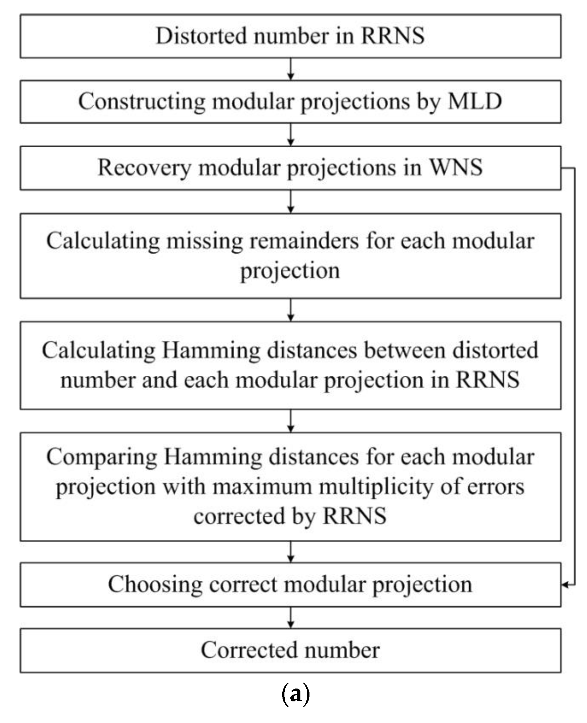
According to [19], each projection is restored in the WNS using the CRT. The resulting projections are employed to calculate the values of the missing remainders. Next, the Hamming distances are calculated for each projection, and the correct projection is selected (Figure 1a).

Figure 1. Modular projection methods with MLD: (a) original, (b) modified.

Reconstructing the weighted representation of projections using the CRT has high time delays. First of all, the delay is due to executing operations on a large modulus comparable to the dynamic range of the RRNS.

In the original method [19], the reconstructed weighted representations of modular projections are used, on the one hand, to calculate the missing remainders subsequently and, on the other hand, to obtain the correct number in the WNS. (One of the projections will be the correct number represented in the WNS.) In the modified method, we propose using (a) the ranks of the modular projections to obtain the missing remainders and (b) the approximate weighted characteristics of the CRTf to restore the modular projections in the WNS. This approach allows for calculating the missing remainders and reconstructing projections in the WNS in parallel (Figure 1b), not sequentially, as was proposed in [19].

The efficiency of the proposed modification largely depends on the efficiency of calculating the rank of a number represented in the RRNS. The choice of the CRTf for reconstructing modular projections in the WNS is not accidental: the approximate weighted characteristic $F\left(X\right)$ closely relates to the rank $r_X$ of the number $X$ written in the RRNS.

According to (3), the rank $r_X$ is given by

$$r_X=\frac{{{\displaystyle \sum }}_{i=1}^k\frac{M_K}{m_i}{\left|\frac{m_i}{M_K}\right|}_{m_i}{x}_i-X}{M_K}=\frac{{{\displaystyle \sum }}_{i=1}^k\frac{M_K}{m_i}{\left|\frac{m_i}{M_K}\right|}_{m_i}{x}_i}{M_K}-\frac{X}{M_K}={\displaystyle \sum }_{i=1}^k\frac{{\left|m_i/M_K\right|}_{m_i}{x}_i}{m_i}-\frac{X}{M_K}.$$

Due to (4) and (5),

$$r_X={\displaystyle \sum }_{i=1}^k\frac{{\left|m_i/M_K\right|}_{m_i}{x}_i}{m_i}-{\left|{\displaystyle \sum }_{i=1}^k\frac{{\left|m_i/M_K\right|}_{m_i}{x}_i}{m_i}\right|}_1.$$

Recall that ${|•|}_1$ denotes taking the fractional part of a number. Hence, the rank of $X$ is given by

$$r_X={\displaystyle ⎣}{{\displaystyle \sum }}_{i=1}^k\frac{{\left|m_i/M_K\right|}_{m_i}{x}_i}{m_i}{\displaystyle ⎦}={\displaystyle ⎣}{{\displaystyle \sum }}_{i=1}^k{k}_i^{*}{x}_i{\displaystyle ⎦},k_i^{*}=\frac{{\left|m_i/M_K\right|}_{m_i}}{m_i}.$$

(10)

Note that $F\left(X\right)$ and $r_X$ are the integer and fractional parts of the same value. We introduce the notation

$$F^{\prime }\left(X\right)={{\displaystyle \sum }}_{i=1}^k{k}_i^{*}{x}_i,k_i^{*}=\frac{{\left|m_i/M_K\right|}_{m_i}}{m_i}.$$

(11)

Calculating $F\prime \left(X\right)$, we simultaneously find the weighted characteristic $F\left(X\right)$ (Equation (5)) and the rank $r_X$ of $X$ (Equation (10)).

Similar to the case of the CRTf (Equations (6) and (7)), we propose using a binary shift to implement the calculation of $F^{\prime }\left(X\right)$ on a hardware base not supporting fractions. The accuracy of the constants $k_i^{*}$ in (11) is estimated by analogy with [20]. Then

$$F^{\prime }\left(X\right)={{\displaystyle \sum }}_{i=1}^k{k}_i^{*}{x}_i,k_i^{*}={\displaystyle ⎡}\frac{{\left|m_i/M_K\right|}_{m_i}}{m_i}\cdot 2^N{\displaystyle ⎤},$$

(12)

where $N=⎡{\log }_2(M_K{{\displaystyle \sum }}_{i=1}^k\left(m_i-1\right))⎤$ [20].

The value $F^{\prime }\left(X\right)$ is especially convenient for the hardware implementation of the error correction procedure for modular codes. Really, the $N$ least significant bits of the binary representation of $F\prime \left(X\right)$ calculated by Equation (12) will be the shifted weighted characteristic $F\left(X\right)$ (Equation (7)):

$$F\left(X\right)=F\prime {(X)}_{\left[N-1..0\right]},$$

(13)

where $N=⎡{\log }_2(M_K{{\displaystyle \sum }}_{i=1}^k\left(m_i-1\right))⎤$ [20].

The other (most significant) bits will be equal to the rank $r_X$ of $X$:

$$r_X=F\prime {(X)}_{\left[Length\left(F^{\prime }\left(X\right)\right)-1..N\right]},$$

(14)

where $N=⎡{\log }_2(M_K{{\displaystyle \sum }}_{i=1}^k\left(m_i-1\right))⎤$ [20].

After obtaining the shifted approximate weighted characteristic $F\left(X\right)$ by Equation (13), the standard CRTf Equation (6) is used for restoration. We discuss in detail the calculation of the missing remainders using the rank $r_X$.

This operation extends the system of RNS moduli [7] and can be performed efficiently by efficiently calculating the rank of a number.

According to (3),

$$X={\displaystyle \sum }_{i=1}^k\frac{M_K}{m_i}{\left|\frac{m_i}{M_K}\right|}_{m_i}{x}_i-r_X{M}_K.$$

Introducing the compact notation $B_i=\frac{M_K}{m_i}{\left|\frac{m_i}{M_K}\right|}_{m_i}$, we write

$$X={\displaystyle \sum }_{i=1}^k{B}_i{x}_i-r_X{M}_K, B_i=\frac{M_K}{m_i}{\left|\frac{m_i}{M_K}\right|}_{m_i}, i=1,\dots k.$$

(15)

Due to (15), for each modular projection, the missing remainders on dividing the number $X$ by the moduli $m_j$ deleted when constructing the projection are given by

$${\left|X\right|}_{m_j}={\left|{\displaystyle \sum }_{i=1}^k{B}_i{x}_i-r_X{M}_K\right|}_{m_j}.$$

Performing trivial transformations, we obtain

$${\left|X\right|}_{m_j}={\left|{\left|{\displaystyle \sum }_{i=1}^k{B}_i{x}_i\right|}_{m_j}+{\left|r_X\cdot \left(-M_K\right)\right|}_{m_j}\right|}_{m_j}$$

and, finally,

$${\left|X\right|}_{m_j}={\left|{\left|{\displaystyle \sum }_{i=1}^k{\left|B_i\right|}_{m_j}{x}_i\right|}_{m_j}+{\left|r_X\cdot {\left|-M_K\right|}_{m_j}\right|}_{m_j}\right|}_{m_j}.$$

(16)

Note that for each modular projection, the values ${\left|B_i\right|}_{m_j}$ and ${\left|-M_K\right|}_{m_j}$ differ. However, these values are completely determined by the set of RRNS moduli. Therefore, they are calculated in advance and stored in the memory of the computing device.

Thus, the missing remainders are calculated using multiplication by a constant and addition on a small modulus comparable to the RRNS moduli. Both operations are well implemented in hardware. The key feature of the proposed approach is the ability to calculate the first term ${\left|{{\displaystyle \sum }}_{i=1}^k{\left|B_i\right|}_{m_j}{x}_i\right|}_{m_j}$ in the sum (16) independently and in parallel with the second one ${\left|r_X\cdot {\left|-M_K\right|}_{m_j}\right|}_{m_j}$. We denote them by $X_{m_j}^{\left(1\right)}$ and $X_{m_j}^{\left(2\right)}$, respectively:

$$X_{m_j}^{\left(1\right)}={\left|{{\displaystyle \sum }}_{i=1}^k{\left|B_i\right|}_{m_j}{x}_i\right|}_{m_j}.$$

(17)

$$X_{m_j}^{\left(2\right)}={\left|r_X\cdot {\left|-M_K\right|}_{m_j}\right|}_{m_j}.$$

(18)

Then Equation (16) becomes

$${\left|X\right|}_{m_j}={\left|X_{m_j}^{\left(1\right)}+X_{m_j}^{\left(2\right)}\right|}_{m_j}.$$

(19)

Since the values $X_{m_j}^{\left(1\right)}$ are calculated in parallel to $F\left(X\right)$ and $X_{m_j}^{\left(2\right)}$, the total execution time of the procedure for correcting errors in modular codes and restoring the correct number in the WNS is reduced.

An example demonstrating an approach to extending the system of RNS moduli using the number rank is presented in Appendix A (See, Example A1).

Another example demonstrating the proposed approach to error correction and restoration of the correct number in the WNS is presented in Appendix B (See, Example A2).

The proposed modified modular projection method with MLD for correcting multiple errors in modular codes allows for achieving a high level of parallelism and significantly reducing the total execution time of the multiple error correction procedure.

The proposed method requires calculation of the rank $r_X$ (Equation (14)) for base extension. CRT-I and CRT-II are not directly applicable to do this, while function $F\left(X\right)$, used in the article, gives the advantage to calculate the relative size of both the value $X$ and $r_X$ simultaneously.

5. Hardware Implementation of Modified Modular Projection Method with MLD

The original [19] and modified modular projection methods for correcting multiple errors in modular codes (Section 4) have the identical error detection stage. For both methods equally, the implementation variability of this stage lies in choosing an appropriate algorithm for calculating the weighted characteristic of the corrected number. The hardware implementation and comparative analysis of such algorithms were presented in [31]. Let us compare the efficiency of error localization and correct data restoration in a WNS.

Using various computing devices for implementing methods and algorithms is often dictated by the need to adapt them to the architectural features of a given hardware base. Support of calculations in the ring of integers is a characteristic feature of FPGA computing devices that increases speed but severely restricts the class of executed tasks.

The original method [19] can be implemented on FPGA without any restrictions. The modified method contains operations with fractions and, therefore, requires adaptation when implemented on FPGA. Equations (12)–(14) are used for passing to integer calculations. This transition is illustrated by an example in Appendix C (See, Example A3).

The result of this example coincides with that of an example in Appendix B. Therefore, the transition to integer calculations by Equations (12)–(14) is correct.

The efficiency of the original [19] and modified methods for correcting multiple errors in modular codes was compared by their implementation in the Very High SpeedIntegrated Circuits Hardware Description Language (VHDL) using Xilinx Vivado 2019.1, a software tool for the design and analysis of HDL structures. For testing, we used a Kintex-7 FPGA (core Xilinx xc7k70tfbg676-2) of a sufficient area without DSP blocks.

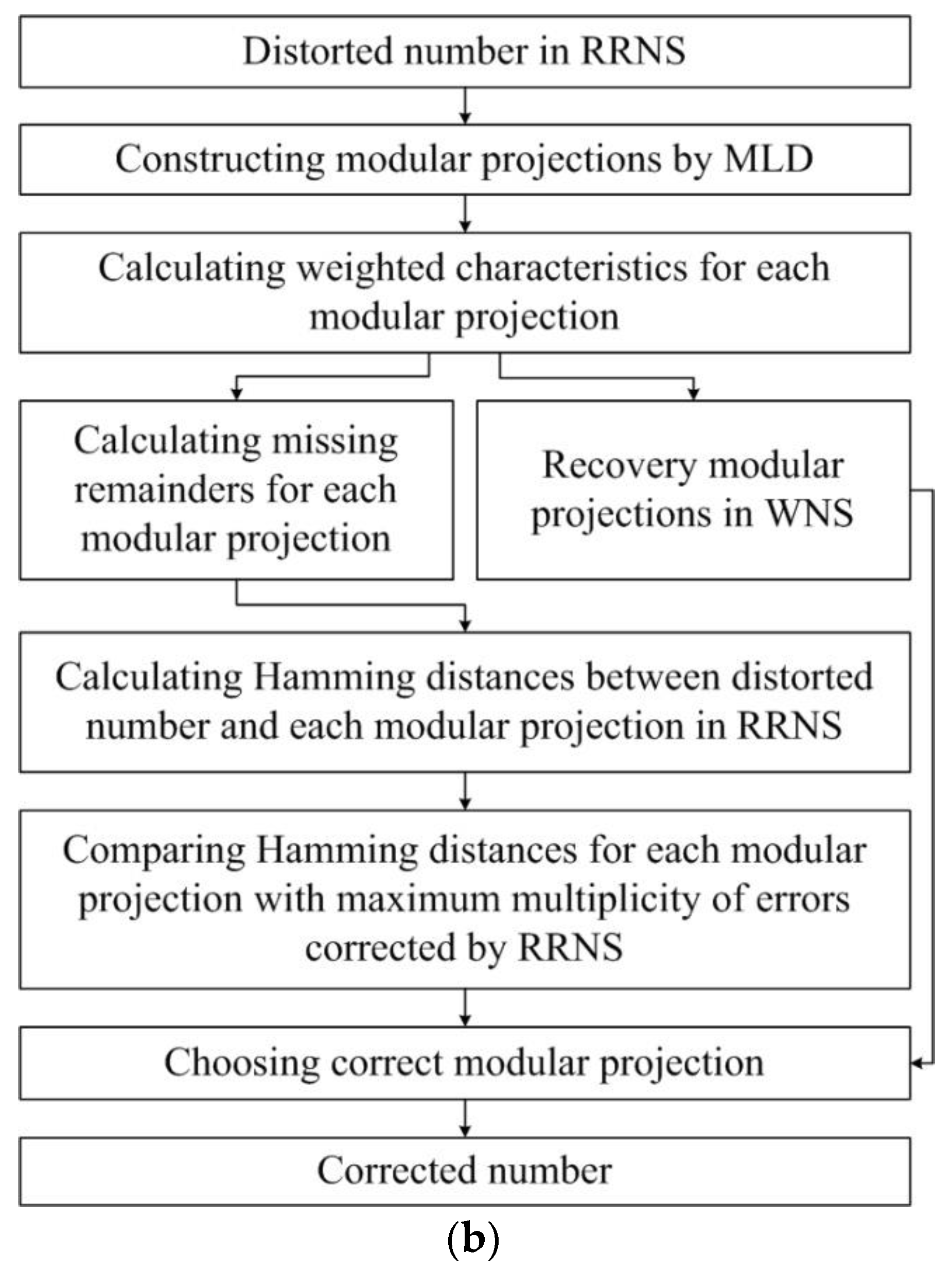
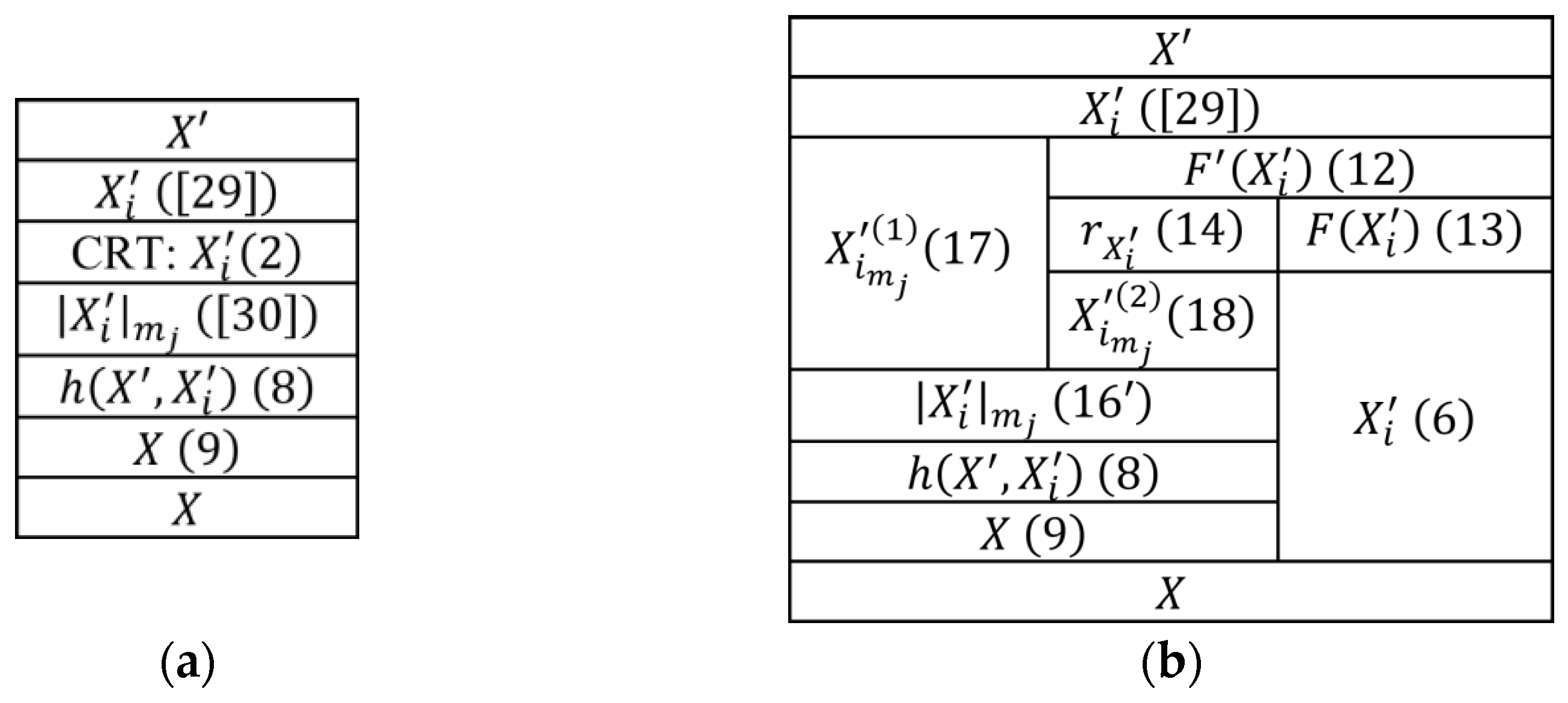
This software–hardware base has hardware parallelization at the level of blocks implementing individual procedures and functions and, moreover, at the level of operations within these blocks. Figure 2 shows the schemes for parallelizing the compared methods at the block level: vertical lines separate parallel executed blocks, whereas horizontal lines indicate the synchronization of upper blocks. The schemes in Figure 2 specify the corresponding schemes in Figure 1, considering their hardware implementation.

Figure 2. Scheme of parallelizing modular projection methods with MLD: (a) original, (b) modified.

The original method [19] contains no parallel blocks (Figure 2a); however, calculations for each modular projection are performed in parallel within each block, except for the first and the last ones. In the modified method, calculations for each modular projection are also performed in parallel within each block, except for the first and last ones; in addition, there is parallelism at the block level (Figure 2b).

Let us consider the hardware implementation of each block in Figure 2.

Original modular projection method with MLD [19] is presented in Appendix D.

Modified Modular Projection Method with MLD

Block $X\prime$. When an error is detected, this block receives at the input $n$ remainders representing the distorted number $X\prime$ in the $\left(n, k\right)$-RRNS.

Block $X_i^{\prime }$. This block constructs modular projections. It is implemented in $C_{⎡n/2⎤}^t$ parallel computational threads, where $t=⎣(n-k)/2⎦$. Each thread corresponds to a modular projection and receives at the input $k$ remainders of the distorted number $X\prime$ (the outputs of the block $X\prime$) obtained by the modular projection algorithm [29].

Block $F\prime \left(X_i^{\prime }\right)$. This block calculates the extended weighted characteristics of modular projections $X_i^{\prime }$ in the WNS. According to (12), it is implemented by $k$ parallel multiplications of the remainders (the outputs of the block $X_i^{\prime }$) by constants modulo $M$ and a $k$-operand adder [31].

Block $r_{X_i^{\prime }}$. This block calculates the ranks for each modular projection $X_i^{\prime }$. It is implemented by extracting the most significant bits with numbers not less than $N$ (14) from the extended weighted characteristic (the output of the block $F^{\prime }\left(X_i^{\prime }\right)$).

Block $F\left(X_i^{\prime }\right)$. This block calculates weighted characteristics for each modular projection $X_i^{\prime }$. It is implemented by extracting the least significant bits with numbers less than $N$ (13) from the extended weighted characteristic (the output of the block $F^{\prime }\left(X_i^{\prime }\right)$).

Block ${X^{\prime }}_{i_{m_j}}^{\left(1\right)}$. This block calculates the missing remainders (the first term) for each modular projection $X_i^{\prime }$. It is implemented by $k$ parallel multiplications of the remainders (the outputs of the block $X_i^{\prime }$) by constants modulo $M$ and a $k$-operand modulo adder [31]; see Equation (17).

Block ${X^{\prime }}_{i_{m_j}}^{\left(2\right)}$. This block calculates the missing remainders (the second term) for each modular projection $X_i^{\prime }$. It is implemented by multiplying the rank (the output of the block $r_{X_i^{\prime }}$) by a constant modulo $M$ [31]; see Equation (18).

Block ${\left|X_i^{\prime }\right|}_{m_j}$. This block calculates the missing remainders for each modular projection $X_i^{\prime }$. It is implemented by modulo adding the first term (the output of the block ${X^{\prime }}_{i_{m_j}}^{\left(1\right)}$) to the second term (the output of the block ${X^{\prime }}_{i_{m_j}}^{\left(2\right)}$) [31]; see Equation (19).

Block $X_i^{\prime }$ (6). This block calculates the modular projections $X_i^{\prime }$ in the WNS. It is implemented by multiplying the weighted characteristic of the modular projection (the output of the block $F\left(X_i^{\prime }\right)$) by the dynamic range $M_K$. Subsequently, the least significant bits with numbers less than $N$ are discarded; see Equation (6).

Block $h\left(X\prime ,X_i^{\prime }\right)$. This block calculates Hamming distances between the distorted number $X\prime$ and each modular projection $X_i^{\prime }$. It is implemented by $\left(n–k\right)$ parallel comparisons of the corresponding remainders of the distorted number $X\prime$ (the outputs of the block $X\prime$) and the modular projection $X_i^{\prime }$ (the outputs of the block ${\left|X_i^{\prime }\right|}_{m_j}$). Subsequently, the mismatches are counted by an $n$-operand adder.

Block $X$X (9). This block chooses a correct modular projection. It is implemented by the conjunction of two comparisons: the modular projection $X_i^{\prime }$ in the WNS (the output of the block CRT: $X_i^{\prime }$) is smaller than the dynamic range $M_K$, and the Hamming distance (the output of the block $h\left(X\prime ,X_i^{\prime }\right)$) is not greater than the maximum multiplicity $t$ of errors corrected by the $\left(n,k\right)$-RRNS. The results for each thread (conjunctions for different modular projections) are glued together into a $C_{⎡n/2⎤}^t$-bit number, and the number of the first nonzero bit corresponds to the correct modular projection.

Block $X$X. This block outputs the correct number $X$ in the WNS. It is implemented by a $C_{⎡n/2⎤}^t$-input multiplexer with one control input. The common inputs are the modular projections $X_i^{\prime }$ in the WNS (the outputs of the block CRT: $X_i^{\prime }$). The control input is the number of the correct modular projection (the output of the block $X$ (9)).

In the course of comparative analysis, we obtained data on the time and hardware costs for correcting single and double errors in modular codes. We used the $\left(2,4\right)$-RRNS (single error) and $\left(2,6\right)$-RRNS (double error) for numbers of different bit widths (4 bits, 8 bits, 16 bits, 24 bits, 32 bits, 48 bits, and 64 bits). The moduli sets, the time and hardware costs for correcting single and double errors and restoring the number in the WNS using the original modular projection method with MLD [19], and the modified one proposed in this paper are presented in Appendix E (See, Table A7 and Table A8).

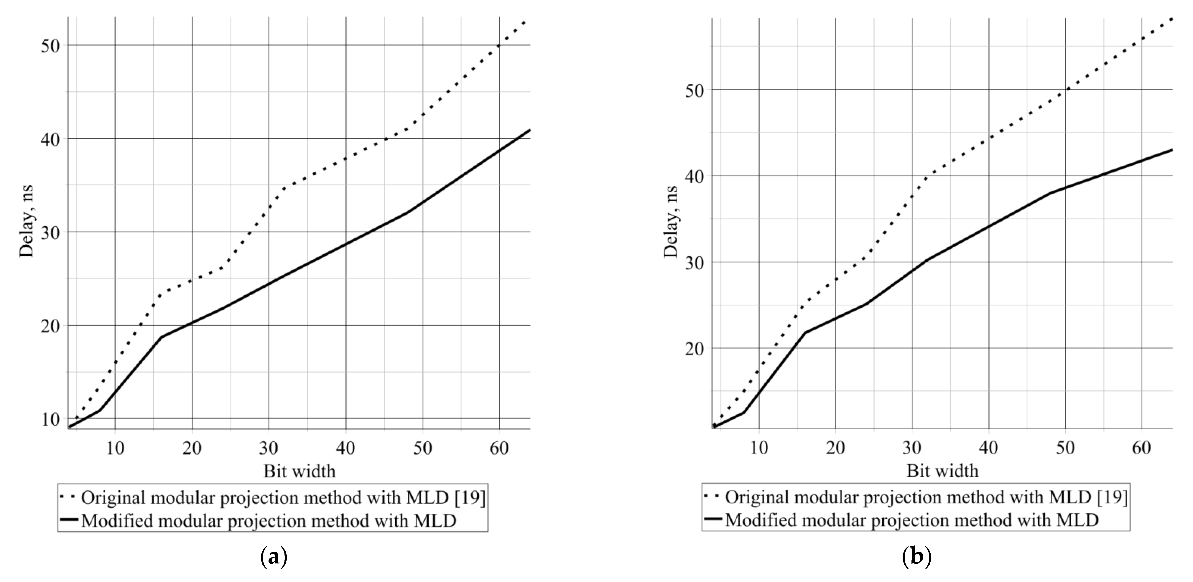
Figure 3 shows the operating times of the methods depending on the bit width of the numbers under correction for a single error (see, Figure 3a) and double errors (see, Figure 3b).

Figure 3. Time to correct errors and restore numbers in WNS: (a) single error, (b) double error.

According to Figure 3, the modified modular projection method with MLD proposed in this dynamic is faster than the original method [19]. Based on the simulation results on FPGA (see Appendix D), we conclude that the proposed method speeds up the procedure of error correction and number restoration in the WNS by an average of 1.23 times (18%) compared to the original approach [19]. On average, the modified modular projection method with MLD requires 1.55 times (35%) more resources for single errors and 1.76 times (43%) more resources for double errors.

6. Conclusions

Recovery weighted values of modular projections has high time complexity due to computations on a large modulus. The paper proposes a method based on the use of approximate positional characteristics and ranks of modular projections. The use of the Chinese Remainder Theorem with fractions in the procedure for correcting errors and recovery numbers in the weighted number system makes it possible to efficiently calculate the rank of each of the modular projections. The ranks of modular projections are employed to calculate the Hamming distances. This approach allows for parallelizing computations at the levels of operations and computing blocks.

The simulation results on FPGA have demonstrated that the proposed modified modular projection method with MLD speeds up the procedure of error correction and number restoration in the weighted number system by an average of 18% compared to the original method [19]. At the same time, it consumes many more hardware resources.

However, in further study, we are going to research the moduli set selection and the possibility of applying the proposed method for error correction codes with the RNS special moduli sets.

Appendix A.1. Base Extension. Pre-Computation Stage

We obtain the constants for the moduli set $\left\{3,5,7\right\}$.

$M_K=m_1{m}_2{m}_3=3\cdot 5\cdot 11=165$.

We calculate the constants$B_i$by Equation (15):

$$B_1=\frac{M_K}{m_1}{\left|\frac{m_1}{M_K}\right|}_{m_1}=\frac{165}{3}{\left|\frac{3}{165}\right|}_3=55\cdot 1=55,$$

$$B_2=\frac{M_K}{m_2}{\left|\frac{m_2}{M_K}\right|}_{m_2}=\frac{165}{5}{\left|\frac{5}{165}\right|}_5=33\cdot 2=66,$$

$$B_3=\frac{M_K}{m_3}{\left|\frac{m_3}{M_K}\right|}_{m_3}=\frac{165}{11}{\left|\frac{11}{165}\right|}_{11}=15\cdot 3=45.$$

Next, we calculate the constants for Equation (16):

$${\left|B_1\right|}_{m_4}={\left|55\right|}_7=6,{\left|B_2\right|}_{m_4}={\left|66\right|}_7=3,{\left|B_3\right|}_{m_4}={\left|45\right|}_7=3,{\left|-M_K\right|}_{m_4}={\left|-165\right|}_7=3.$$

Finally, we calculate the constants necessary for finding the rank $r_X$ of $X$. According to (10),

$$k_1^{*}=\frac{{\left|m_1/M_K\right|}_{m_1}}{m_1}=\frac{{\left|3/165\right|}_3}{3}=\frac{1}{3},$$

$$k_2^{*}=\frac{{\left|m_2/M_K\right|}_{m_2}}{m_2}=\frac{{\left|5/165\right|}_5}{5}=\frac{2}{5},$$

$$k_3^{*}=\frac{{\left|m_3/M_K\right|}_{m_3}}{m_3}=\frac{{\left|11/165\right|}_{11}}{11}=\frac{3}{11}.$$

Appendix A.2. Base Extension. Computation Stage

Step 1. We obtain $X_{m_4}^{\left(1\right)}$ by Equation (17):

$$X_{m_4}^{\left(1\right)}={\left|{{\displaystyle \sum }}_{i=1}^3{\left|B_i\right|}_{m_4}{x}_i\right|}_{m_4}={\left|6\cdot 1+3\cdot 4+3\cdot 6\right|}_7=1.$$

Calculating the first term in Equation (16), we calculate the rank $r_X$ in parallel. According to (10),

$$r_X=⎣{\displaystyle \sum }_{i=1}^3{k}_i^{*}{x}_i⎦=⎣\frac{1}{3}\cdot 1+\frac{2}{5}\cdot 4+\frac{3}{11}\cdot 6⎦=⎣3\frac{94}{165}⎦=3.$$

Using Equation (18), we find the second term $X_{m_4}^{\left(2\right)}$ in Equation (16):

$$X_{m_4}^{\left(2\right)}={\left|r_X\cdot {\left|-M_K\right|}_{m_4}\right|}_{m_4}={\left|3\cdot 3\right|}_7=2.$$

Step 2. We calculate the desired remainder by Equation (19):

$${\left|X\right|}_{m_4}={\left|X_{m_4}^{\left(1\right)}+X_{m_4}^{\left(2\right)}\right|}_{m_4}={\left|1+2\right|}_7=3.$$

This value matches the remainder on dividing $X=94$ by the modulus $m_4=7$.

End of example.

Appendix B.1. Error Detection. Pre-Computation Stage

To detect an error, we have to restore the number $X\prime$ in the WNS and compare it with the dynamic range $M_K$ or calculate the weighted characteristic $F\left(X\prime \right)$ and compare it with the corresponding weighted characteristic $F\left(M_K\right)$ of the dynamic range. To reduce calculations, we detect errors using weighted characteristics yielded by the CRTf. We calculate all necessary constants that can be pre-computed, saving them in memory (See, Table A1).

We calculate the dynamic and full ranges of this RRNS:

$$M_K=5·7=35, M_N=5·7·8·9·11·13=360360.$$

The constants for error detection (Equation (5)) are

$$k_1^{*}=\frac{{\left|m_1/M_N\right|}_{m_1}}{m_1}=\frac{{\left|5/360360\right|}_5}{5}=\frac{3}{5},$$

$$k_2^{*}=\frac{{\left|m_2/M_N\right|}_{m_2}}{m_2}=\frac{{\left|7/360360\right|}_7}{7}=\frac{4}{7},$$

$$k_3^{*}=\frac{{\left|m_3/M_N\right|}_{m_3}}{m_3}=\frac{{\left|8/360360\right|}_8}{8}=\frac{5}{8},$$

$$k_4^{*}=\frac{{\left|m_4/M_N\right|}_{m_4}}{m_4}=\frac{{\left|9/360360\right|}_9}{9}=\frac{8}{9},$$

$$k_5^{*}=\frac{{\left|m_5/M_N\right|}_{m_5}}{m_5}=\frac{{\left|11/360360\right|}_{11}}{11}=\frac{6}{11},$$

$$k_6^{*}=\frac{{\left|m_6/M_N\right|}_{m_6}}{m_6}=\frac{{\left|13/360360\right|}_{13}}{13}=\frac{10}{13}.$$

According to Equation (4),

$$F\left(M_K\right)=\frac{M_K}{M_N}=\frac{35}{360360}=\frac{1}{10296}.$$

Table A1. Pre-computed constants for error detection using CRTf.

$\left\{{\mathit{m}}_{\mathit{i}}\right\}$	$\left\{{\mathit{k}}_{\mathit{i}}^{*}\right\}$	$\mathit{F}\left({\mathit{M}}_{\mathit{K}}\right)$
$\left\{5, 7, 8, 9, 11, 13\right\}$	$\left\{3/5, 4/7, 5/8, 8/9, 6/11, 10/13\right\}$	$1/10296$

Table A1. Pre-computed constants for error detection using CRTf.

$\left\{{\mathit{m}}_{\mathit{i}}\right\}$	$\left\{{\mathit{k}}_{\mathit{i}}^{*}\right\}$	$\mathit{F}\left({\mathit{M}}_{\mathit{K}}\right)$
$\left\{5, 7, 8, 9, 11, 13\right\}$	$\left\{3/5, 4/7, 5/8, 8/9, 6/11, 10/13\right\}$	$1/10296$

Appendix B.2. Error Detection. Computation Stage

According to Equation (5),

$$\begin{gathered} F\left(X\prime \right)={\left|{\displaystyle \sum }_{i=1}^6{k}_i^{*}{x}_i^{\prime }\right|}_1={\left|\frac{3}{5}\cdot 0+\frac{4}{7}\cdot 3+\frac{5}{8}\cdot 7+\frac{8}{9}\cdot 6+\frac{6}{11}\cdot 1+\frac{10}{13}\cdot 2\right|}_1= \\ ={\left|\frac{324481}{24024}\right|}_1=\frac{12169}{24024}\ge \frac{1}{10296}=F\left(M_K\right). \end{gathered}$$

Since $F\left(X\prime \right)\ge F\left(M_K\right)$, the number$X\prime$contains an error.

Appendix B.3. Error Localization and Correction. Pre-Computation Stage

To correct errors, we use the modified modular projection method with MLD. The projections are constructed according to the algorithm [29]:

$$X_{1,2}^{\prime }=\left(x_1,x_2,x_3,x_4,x_5,x_6\right),$$

$$X_{3,4}^{\prime }=\left(x_1,x_2,x_3,x_4,x_5,x_6\right),$$

$$X_{5,6}^{\prime }=\left(x_1,x_2,x_3,x_4,x_5,x_6\right).$$

We calculate constants for each modular projection, saving them in memory (See, Table A2).

Table A2. Pre-computed constants for each modular projection.

		Modular Projection
		${\mathit{X}}_{1,2}^{\prime }=\left\{0, 3\right\}$	${\mathit{X}}_{3,4}^{\prime }=\left\{7, 6\right\}$	${\mathit{X}}_{5,6}^{\prime }=\left\{1, 2\right\}$
1	Number	$i=1, 2$ $j=3,\dots ,6$	$i=3, 4$ $j=1, 2, 5, 6$	$i=5, 6$ $j=1,\dots , 4$
2	$\left\{m_i\right\}$	$\left\{5, 7\right\}$	$\left\{8, 9\right\}$	$\left\{11, 13\right\}$
3	$M_K$	$35$	$72$	$143$
4	$F\left(M_K\right), \left(M_K=35\right)$	$1$	$35/72$	$35/143$
5	$\left\{k_i^{*}\right\}$	$\left\{3/5, 3/7\right\}$	$\left\{1/8, 8/9\right\}$	$\left\{6/11, 6/13\right\}$
6	$[\{{\left|B_i\right|}_{m_j}$}]	$\left[\left\{5, 7\right\}, \left\{3, 6\right\}, \left\{10, 4\right\},\left\{8, 2\right\}\right]$	$\left[\left\{4, 4\right\}, \left\{2, 1\right\}, \left\{9, 9\right\},\left\{9, 12\right\}\right]$	$\left[\left\{3, 1\right\}, \left\{1, 3\right\}, \left\{6, 2\right\}, \left\{6, 3\right\}\right]$
7	$\{{\left|-M_K\right|}_{m_j}$}	$\left\{5, 1, 9, 4\right\}$	$\left\{3, 5, 5, 6\right\}$	$\left\{2, 4, 1, 1\right\}$

Table A2. Pre-computed constants for each modular projection.

		Modular Projection
		${\mathit{X}}_{1,2}^{\prime }=\left\{0, 3\right\}$	${\mathit{X}}_{3,4}^{\prime }=\left\{7, 6\right\}$	${\mathit{X}}_{5,6}^{\prime }=\left\{1, 2\right\}$
1	Number	$i=1, 2$ $j=3,\dots ,6$	$i=3, 4$ $j=1, 2, 5, 6$	$i=5, 6$ $j=1,\dots , 4$
2	$\left\{m_i\right\}$	$\left\{5, 7\right\}$	$\left\{8, 9\right\}$	$\left\{11, 13\right\}$
3	$M_K$	$35$	$72$	$143$
4	$F\left(M_K\right), \left(M_K=35\right)$	$1$	$35/72$	$35/143$
5	$\left\{k_i^{*}\right\}$	$\left\{3/5, 3/7\right\}$	$\left\{1/8, 8/9\right\}$	$\left\{6/11, 6/13\right\}$
6	$[\{{\left|B_i\right|}_{m_j}$}]	$\left[\left\{5, 7\right\}, \left\{3, 6\right\}, \left\{10, 4\right\},\left\{8, 2\right\}\right]$	$\left[\left\{4, 4\right\}, \left\{2, 1\right\}, \left\{9, 9\right\},\left\{9, 12\right\}\right]$	$\left[\left\{3, 1\right\}, \left\{1, 3\right\}, \left\{6, 2\right\}, \left\{6, 3\right\}\right]$
7	$\{{\left|-M_K\right|}_{m_j}$}	$\left\{5, 1, 9, 4\right\}$	$\left\{3, 5, 5, 6\right\}$	$\left\{2, 4, 1, 1\right\}$

The modular projection $X_{1,2}^{\prime }: \left\{m_i\right\}=\left\{m_1,m_2\right\}=\left\{5,7\right\}$, $M_K=5·7=35$.

The weighted characteristic of the dynamic range$M_K$for the projection is obtained by Equation (4):

$$F\left(35\right)=35/M_K=35/35=1.$$

The constants for Equation (18) are

$${\left|-M_K\right|}_{m_3}={\left|-35\right|}_8=5,{\left|-M_K\right|}_{m_4}={\left|-35\right|}_9=1,$$

$${\left|-M_K\right|}_{m_5}={\left|-35\right|}_{11}=9,{\left|-M_K\right|}_{m_6}={\left|-35\right|}_{13}=4.$$

According to Equation (15),

$$B_1=\frac{M_K}{m_1}{\left|\frac{m_1}{M_K}\right|}_{m_1}=\frac{35}{5}{\left|\frac{5}{35}\right|}_5=7\cdot 3=21,$$

$$B_2=\frac{M_K}{m_2}{\left|\frac{m_2}{M_K}\right|}_{m_2}=\frac{35}{7}{\left|\frac{7}{35}\right|}_7=5\cdot 3=15.$$

The constants for Equation (17) are

$${\left|B_1\right|}_{m_3}={\left|21\right|}_8=5,{\left|B_1\right|}_{m_4}={\left|21\right|}_9=3,{\left|B_1\right|}_{m_5}={\left|21\right|}_{11}=10,{\left|B_1\right|}_{m_6}={\left|21\right|}_{13}=8,$$

$${\left|B_2\right|}_{m_3}={\left|15\right|}_8=7,{\left|B_2\right|}_{m_4}={\left|15\right|}_9=6,{\left|B_2\right|}_{m_5}={\left|15\right|}_{11}=4,{\left|B_2\right|}_{m_6}={\left|15\right|}_{13}=2.$$

According to (11),

$$k_1^{*}=\frac{{\left|m_1/M_K\right|}_{m_1}}{m_1}=\frac{{\left|5/35\right|}_5}{5}=\frac{3}{5},$$

$$k_2^{*}=\frac{{\left|m_2/M_K\right|}_{m_2}}{m_2}=\frac{{\left|7/35\right|}_7}{7}=\frac{3}{7}.$$

The modular projection$X_{3,4}^{\prime }: \left\{m_i\right\}=\left\{m_3, m_4\right\}=\left\{8, 9\right\}$,$M_K=8·9=72$.

The weighted characteristic of the dynamic range$M_K$for the projection is obtained by Equation (4):

$$F\left(35\right)=35/M_K=35/72.$$

The constants for Equation (18) are

$${\left|-M_K\right|}_{m_1}={\left|-72\right|}_5=3,{\left|-M_K\right|}_{m_2}={\left|-72\right|}_7=5,$$

$${\left|-M_K\right|}_{m_5}={\left|-72\right|}_{11}=5,{\left|-M_K\right|}_{m_6}={\left|-72\right|}_{13}=6.$$

According to Equation (15),

$$B_3=\frac{M_K}{m_3}{\left|\frac{m_3}{M_K}\right|}_{m_3}=\frac{72}{8}{\left|\frac{8}{72}\right|}_8=9\cdot 1=9,$$

$$B_4=\frac{M_K}{m_4}{\left|\frac{m_4}{M_K}\right|}_{m_4}=\frac{72}{9}{\left|\frac{9}{72}\right|}_9=8\cdot 8=64.$$

The constants for Equation (17) are

$${\left|B_3\right|}_{m_1}={\left|9\right|}_5=4,{\left|B_3\right|}_{m_2}={\left|9\right|}_7=2,{\left|B_3\right|}_{m_5}={\left|9\right|}_{11}=9,{\left|B_3\right|}_{m_6}={\left|9\right|}_{13}=9,$$

$${\left|B_4\right|}_{m_1}={\left|64\right|}_5=4,{\left|B_4\right|}_{m_2}={\left|64\right|}_7=1,{\left|B_4\right|}_{m_5}={\left|64\right|}_{11}=9,{\left|B_4\right|}_{m_6}={\left|64\right|}_{13}=12.$$

According to (11),

$$k_3^{*}=\frac{{\left|m_3/M_K\right|}_{m_3}}{m_3}=\frac{{\left|8/72\right|}_8}{8}=\frac{1}{8},$$

$$k_4^{*}=\frac{{\left|m_4/M_K\right|}_{m_4}}{m_4}=\frac{{\left|9/72\right|}_9}{9}=\frac{8}{9}.$$

The modular projection$X_{5,6}^{\prime }: \left\{m_i\right\}=\left\{m_5, m_6\right\}=\left\{11, 13\right\}$,$M_K=11·13=143$.

The weighted characteristic of the dynamic range$M_K$for the projection is obtained by Equation (4):

$$F\left(35\right)=35/M_K=35/143.$$

The constants for Equation (18) are

$${\left|-M_K\right|}_{m_1}={\left|-143\right|}_5=2,{\left|-M_K\right|}_{m_2}={\left|-143\right|}_7=4,$$

$${\left|-M_K\right|}_{m_3}={\left|-143\right|}_8=1,{\left|-M_K\right|}_{m_4}={\left|-143\right|}_9=1.$$

According to Equation (15),

$$B_5=\frac{M_K}{m_5}{\left|\frac{m_5}{M_K}\right|}_{m_5}=\frac{143}{11}{\left|\frac{11}{143}\right|}_{11}=13\cdot 6=78,$$

$$B_6=\frac{M_K}{m_6}{\left|\frac{m_6}{M_K}\right|}_{m_6}=\frac{143}{13}{\left|\frac{13}{143}\right|}_{13}=11\cdot 6=66.$$

The constants for Equation (17) are

$${\left|B_5\right|}_{m_1}={\left|78\right|}_5=3,{\left|B_5\right|}_{m_2}={\left|78\right|}_7=1,{\left|B_5\right|}_{m_3}={\left|78\right|}_8=6,{\left|B_5\right|}_{m_4}={\left|78\right|}_9=6,$$

$${\left|B_6\right|}_{m_1}={\left|66\right|}_5=1,{\left|B_6\right|}_{m_2}={\left|66\right|}_7=3,{\left|B_6\right|}_{m_3}={\left|66\right|}_8=2,{\left|B_6\right|}_{m_4}={\left|66\right|}_9=3.$$

According to (11),

$$k_5^{*}=\frac{{\left|m_5/M_K\right|}_{m_5}}{m_5}=\frac{{\left|11/143\right|}_{11}}{11}=\frac{6}{11},$$

$$k_6^{*}=\frac{{\left|m_6/M_K\right|}_{m_6}}{m_6}=\frac{{\left|13/143\right|}_{13}}{13}=\frac{6}{13}.$$

Appendix B.4. Error Localization and Correction. Computation Stage

Step 1. We calculate the extended weighted characteristic for each modular projection (Equation (11)) using the pre-computed constants from Table A2. The weighted characteristic and rank of each modular projection are the fractional and integer parts, respectively, of the extended weighted characteristic.

The modular projection$X_{1,2}^{\prime }$:

$$F\prime \left(X_{1,2}^{\prime }\right)=\frac{3}{5}\cdot 0+\frac{3}{7}\cdot 3=1\frac{2}{7},$$

$$F\left(X_{1,2}^{\prime }\right)={\left|F\prime \left(X_{1,2}^{\prime }\right)\right|}_1={\left|1\frac{2}{7}\right|}_1=\frac{2}{7},r_{X_{1,2}^{\prime }}=⎣F\prime \left(X_{1,2}^{\prime }\right)⎦=⎣1\frac{2}{7}⎦=1.$$

The modular projection$X_{3,4}^{\prime }$:

$$F\prime \left(X_{3,4}^{\prime }\right)=\frac{1}{8}\cdot 7+\frac{8}{9}\cdot 6=6\frac{5}{24},$$

$$F\left(X_{3,4}^{\prime }\right)={\left|F\prime \left(X_{3,4}^{\prime }\right)\right|}_1={\left|6\frac{5}{24}\right|}_1=\frac{5}{24},r_{X_{3,4}^{\prime }}=⎣F\prime \left(X_{3,4}^{\prime }\right)⎦=⎣6\frac{5}{24}⎦=6.$$

The modular projection$X_{5,6}^{\prime }$:

$$F\prime \left(X_{5,6}^{\prime }\right)=\frac{6}{11}\cdot 1+\frac{6}{13}\cdot 2=1\frac{67}{143},$$

$$F\left(X_{5,6}^{\prime }\right)={\left|F\prime \left(X_{5,6}^{\prime }\right)\right|}_1={\left|1\frac{67}{143}\right|}_1=\frac{67}{143},r_{X_{5,6}^{\prime }}=⎣F\prime \left(X_{5,6}^{\prime }\right)⎦=⎣1\frac{67}{143}⎦=1.$$

Step 2. We calculate the second terms for finding the missing remainders for each modular projection (Equation (18)) using the constants from Table A2.

The modular projection$X_{1,2}^{\prime }$:

$${X^{\prime }}_{1,2m_3}^{\left(2\right)}={\left|1\cdot 5\right|}_8=5,{X^{\prime }}_{1,2m_4}^{\left(2\right)}={\left|1\cdot 1\right|}_9=1,$$

$${X^{\prime }}_{1,2m_5}^{\left(2\right)}={\left|1\cdot 9\right|}_{11}=9,{X^{\prime }}_{1,2m_6}^{\left(2\right)}={\left|1\cdot 4\right|}_{13}=4.$$

The modular projection$X_{3,4}^{\prime }$:

$${X^{\prime }}_{3,4m_1}^{\left(2\right)}={\left|6\cdot 3\right|}_5=3,{X^{\prime }}_{3,4m_2}^{\left(2\right)}={\left|6\cdot 5\right|}_7=2,$$

$${X^{\prime }}_{3,4m_5}^{\left(2\right)}={\left|6\cdot 5\right|}_{11}=8,{X^{\prime }}_{3,4m_6}^{\left(2\right)}={\left|6\cdot 6\right|}_{13}=10.$$

The modular projection$X_{5,6}^{\prime }$:

$${X^{\prime }}_{5,6m_1}^{\left(2\right)}={\left|1\cdot 2\right|}_5=2,{X^{\prime }}_{5,6m_2}^{\left(2\right)}={\left|1\cdot 4\right|}_7=4,$$

$${X^{\prime }}_{5,6m_3}^{\left(2\right)}={\left|1\cdot 1\right|}_8=1,{X^{\prime }}_{5,6m_4}^{\left(2\right)}={\left|1\cdot 1\right|}_9=1.$$

We obtain the weighted representations of modular projections (Equation (4)) in parallel with calculating the second terms.

The modular projection$X_{1,2}^{\prime }$:

$$X_{1,2}^{\prime }=F\left(X_{1,2}^{\prime }\right)M_K=\frac{2}{7}\cdot 35=10.$$

The modular projection$X_{3,4}^{\prime }$:

$$X_{3,4}^{\prime }=F\left(X_{3,4}^{\prime }\right)M_K=\frac{5}{24}\cdot 72=15.$$

The modular projection$X_{5,6}^{\prime }$:

$$X_{5,6}^{\prime }=F\left(X_{5,6}^{\prime }\right)M_K=\frac{67}{143}\cdot 143=67.$$

Step (1–2). We calculate the first terms for finding the missing remainders for each modular projection (Equation (17)) using the constants from Table A2. This is done in parallel with Steps 1–2.

The modular projection$X_{1,2}^{\prime }$:

$${X^{\prime }}_{1,2m_3}^{\left(1\right)}={\left|5\cdot 0+7\cdot 3\right|}_8=5,{X^{\prime }}_{1,2m_4}^{\left(1\right)}={\left|3\cdot 0+6\cdot 3\right|}_9=0,$$

$${X^{\prime }}_{1,2m_5}^{\left(1\right)}={\left|10\cdot 0+4\cdot 3\right|}_{11}=1,{X^{\prime }}_{1,2m_6}^{\left(1\right)}={\left|8\cdot 0+2\cdot 3\right|}_{13}=6.$$

The modular projection$X_{3,4}^{\prime }$:

$${X^{\prime }}_{3,4m_1}^{\left(1\right)}={\left|4\cdot 7+4\cdot 6\right|}_5=2,{X^{\prime }}_{3,4m_2}^{\left(1\right)}={\left|2\cdot 7+1\cdot 6\right|}_7=6,$$

$${X^{\prime }}_{3,4m_5}^{\left(1\right)}={\left|9\cdot 7+9\cdot 6\right|}_{11}=7,{X^{\prime }}_{3,4m_6}^{\left(1\right)}={\left|9\cdot 7+12\cdot 6\right|}_{13}=5.$$

The modular projection$X_{5,6}^{\prime }$:

$${X^{\prime }}_{5,6m_1}^{\left(1\right)}={\left|3\cdot 1+1\cdot 2\right|}_5=0,{X^{\prime }}_{5,6m_2}^{\left(1\right)}={\left|1\cdot 1+3\cdot 2\right|}_7=0,$$

$${X^{\prime }}_{5,6m_3}^{\left(1\right)}={\left|6\cdot 1+2\cdot 2\right|}_8=2,{X^{\prime }}_{5,6m_4}^{\left(1\right)}={\left|6\cdot 1+3\cdot 2\right|}_9=3.$$

Step 3. We calculate the missing remainders for each modular projection (Equation (19)).

The modular projection$X_{1,2}^{\prime }$:

$${\left|X_{1,2}^{\prime }\right|}_{m_3}={\left|5+5\right|}_8=2,{\left|X_{1,2}^{\prime }\right|}_{m_4}={\left|0+1\right|}_9=1,$$

$${\left|X_{1,2}^{\prime }\right|}_{m_5}={\left|1+9\right|}_{11}=10,{\left|X_{1,2}^{\prime }\right|}_{m_6}={\left|6+4\right|}_{13}=10.$$

The modular projection$X_{3,4}^{\prime }$:

$${\left|X_{3,4}^{\prime }\right|}_{m_1}={\left|2+3\right|}_5=0,{\left|X_{3,4}^{\prime }\right|}_{m_2}={\left|6+2\right|}_7=1,$$

$${\left|X_{3,4}^{\prime }\right|}_{m_5}={\left|7+8\right|}_{11}=4,{\left|X_{3,4}^{\prime }\right|}_{m_6}={\left|5+10\right|}_{13}=2.$$

The modular projection$X_{5,6}^{\prime }$:

$${\left|X_{5,6}^{\prime }\right|}_{m_1}={\left|0+2\right|}_5=2,{\left|X_{5,6}^{\prime }\right|}_{m_2}={\left|0+4\right|}_7=4,$$

$${\left|X_{5,6}^{\prime }\right|}_{m_3}={\left|2+1\right|}_8=3,{\left|X_{5,6}^{\prime }\right|}_{m_4}={\left|3+1\right|}_9=4.$$

Step 4. We calculate the Hamming distances between each modular projection in the RRNS and the distorted number (Equation (8)):

$$h\left(X^{\prime },X_{1,2}^{\prime }\right)=h\left(\begin{array}{c}\left(0,3,7,6,1,2\right)\\ \left(0,3,2,1,10,10\right)\end{array}\right)=4,$$

$$h\left(X^{\prime },X_{3,4}^{\prime }\right)=h\left(\begin{array}{c}\left(0,3,7,6,1,2\right)\\ \left(0,1,7,6,4,2\right)\end{array}\right)=2,$$

$$h\left(X^{\prime },X_{5,6}^{\prime }\right)=h\left(\begin{array}{c}\left(0,3,7,6,1,2\right)\\ \left(2,4,3,4,1,2\right)\end{array}\right)=4.$$

Step 5. We choose a correct projection (See, Table A3).

Table A3. Computed modular projections and their characteristics.

		Modular Projection
		${\mathit{X}}_{1,2}^{\prime }=10$	${\mathit{X}}_{3,4}^{\prime }=15$	${\mathit{X}}_{5,6}^{\prime }=67$
1	$F\left(X_i^{\prime }\right)$	2/7	5/24	67/143
2	$F\left(M_K\right)$$,(M_K=35$)	1	35/72	35/143
3	$\left(x_i^{\prime }\right)$	(0,3,2,1,10,10)	(0,1,7,6,4,2)	(2,4,3,4,1,2)
4	$\left(x\prime \right)$	(0,3,7,6,1,2)	(0,3,7,6,1,2)	(0,3,7,6,1,2)
5	$h\left(X\prime ,X_i^{\prime }\right)$	4	2	4
6	$F\left(X_i^{\prime }\right)<F\left(M_K\right)$$,\left(M_K=35\right)$	Yes	Yes	No
7	$h\left(X\prime ,X_i^{\prime }\right)\le t, \left(t=2\right)$	No	Yes	No

Table A3. Computed modular projections and their characteristics.

		Modular Projection
		${\mathit{X}}_{1,2}^{\prime }=10$	${\mathit{X}}_{3,4}^{\prime }=15$	${\mathit{X}}_{5,6}^{\prime }=67$
1	$F\left(X_i^{\prime }\right)$	2/7	5/24	67/143
2	$F\left(M_K\right)$$,(M_K=35$)	1	35/72	35/143
3	$\left(x_i^{\prime }\right)$	(0,3,2,1,10,10)	(0,1,7,6,4,2)	(2,4,3,4,1,2)
4	$\left(x\prime \right)$	(0,3,7,6,1,2)	(0,3,7,6,1,2)	(0,3,7,6,1,2)
5	$h\left(X\prime ,X_i^{\prime }\right)$	4	2	4
6	$F\left(X_i^{\prime }\right)<F\left(M_K\right)$$,\left(M_K=35\right)$	Yes	Yes	No
7	$h\left(X\prime ,X_i^{\prime }\right)\le t, \left(t=2\right)$	No	Yes	No

Both correctness conditions (9) are satisfied for the modular projection$X_{3,4}^{\prime }$only. Therefore, the corrected number is$X=X_{3,4}^{\prime }=15=\left(0, 1, 7, 6, 4, 2\right)$, and the proposed error correction method works properly.

End of example.