
Describing a Set of Points with Elliptical Areas: Mathematical Description and Verification on Operational Tests of Technical Devices


Abstract
1. Introduction
2. Materials and Methods
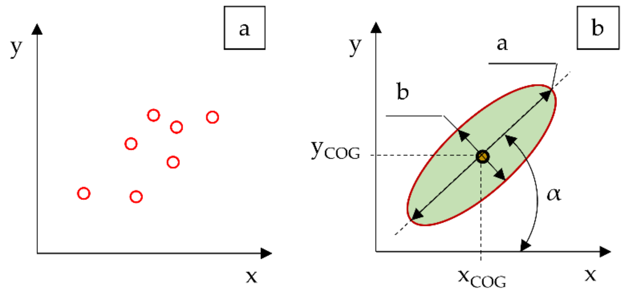
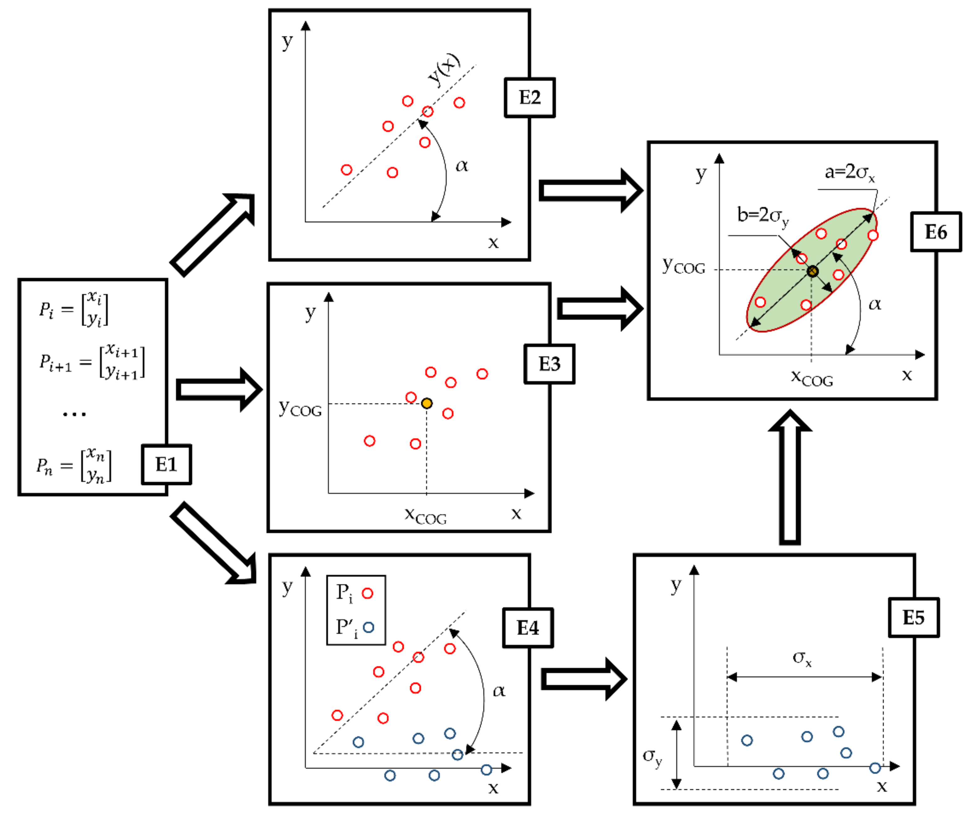
2.1. Mathematical Description of the Method
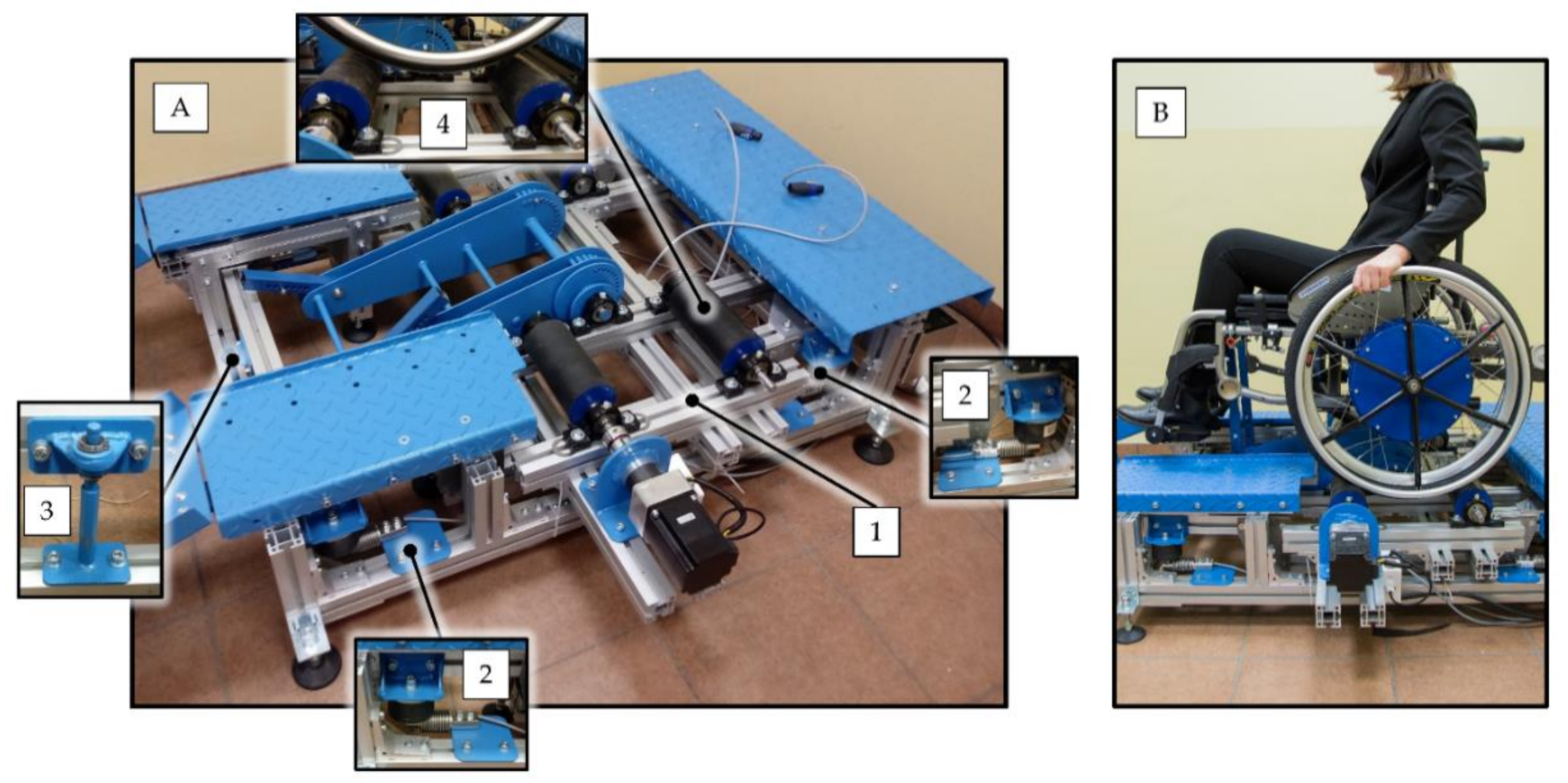
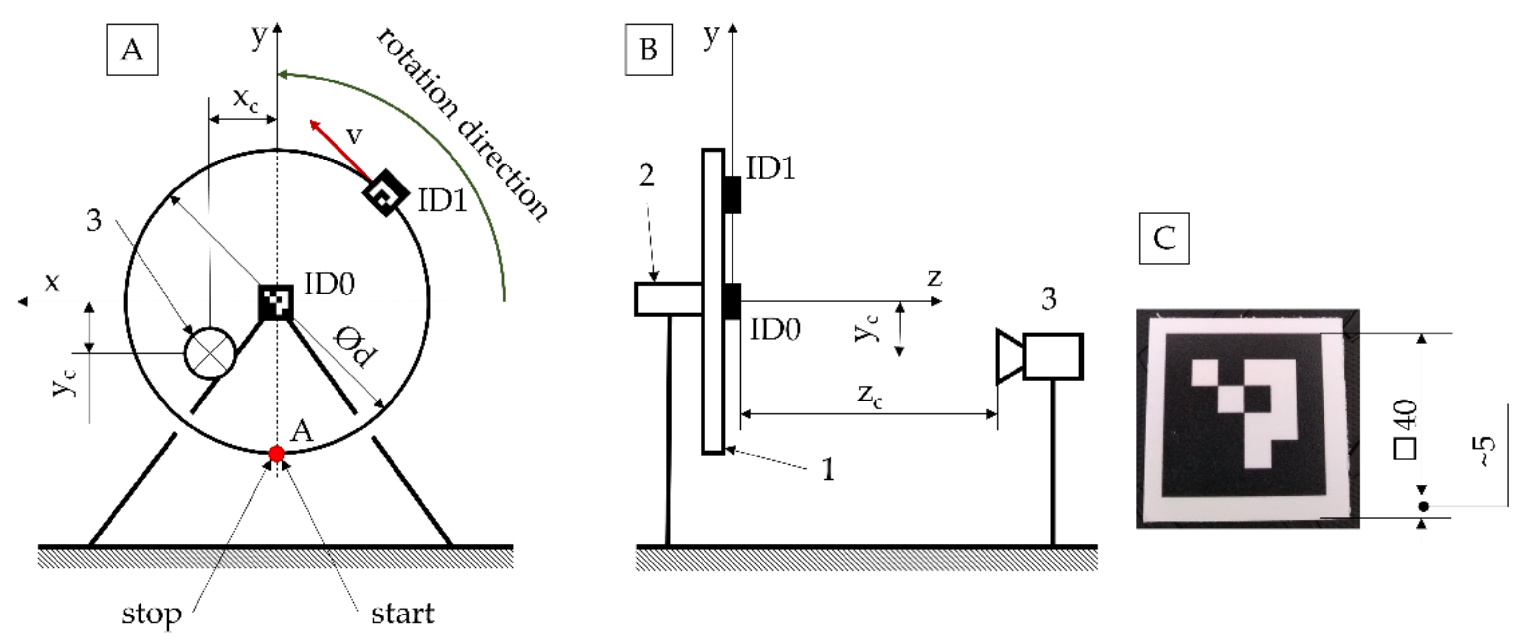
2.2. Procedures for the Verification of the Method
3. Results
4. Discussion
5. Conclusions
Author Contributions
Funding
Institutional Review Board Statement
Informed Consent Statement
Data Availability Statement
Conflicts of Interest
References
- Krawiec, P.; Warguła, Ł.; Małozięć, D.; Kaczmarzyk, P.; Dziechciarz, A.; Czarnecka-Komorowska, D. The Toxicological Testing and Thermal Decomposition of Drive and Transport Belts Made of Thermoplastic Multilayer Polymer Materials. Polymers 2020, 12, 2232. [Google Scholar] [CrossRef] [PubMed]
- Krawiec, P.; Różański, L.; Czarnecka-Komorowska, D.; Warguła, Ł. Evaluation of the thermal stability and surface characteristics of thermoplastic polyurethane V-belt. Materials 2020, 13, 1502. [Google Scholar] [CrossRef]
- Sydor, M. Geometry of wood screws: A patent review. Eur. J. Wood Wood Prod. 2019, 77, 93–103. [Google Scholar] [CrossRef]
- Rui, J.; Gao, Q. Design and Analysis of A Multifunctional Wheelchair. In IOP Conference Series: Materials Science and Engineering; IOP Publishing: Bristol, UK, 2019; Volume 538, p. 12045. [Google Scholar]
- Rebsamen, B.; Guan, C.; Zhang, H.; Wang, C.; Teo, C.; Ang, M.H.; Burdet, E. A brain controlled wheelchair to navigate in familiar environments. IEEE Trans. Neural Syst. Rehabil. Eng. 2010, 18, 590–598. [Google Scholar] [CrossRef]
- Tanaka, K.; Matsunaga, K.; Wang, H.O. Electroencephalogram-based control of an electric wheelchair. IEEE Trans. Robot. 2005, 21, 762–766. [Google Scholar] [CrossRef]
- Minav, T.A.; Heikkinen, J.E.; Pietola, M. Direct driven hydraulic drive for new powertrain topologies for non-road mobile machinery. Electr. Power Syst. Res. 2017, 152, 390–400. [Google Scholar] [CrossRef]
- Lajunen, A.; Sainio, P.; Laurila, L.; Pippuri-Mäkeläinen, J.; Tammi, K. Overview of powertrain electrification and future scenarios for non-road mobile machinery. Energies 2018, 11, 1184. [Google Scholar] [CrossRef]
- Čižiūnienė, K.; Matijošius, J.; Čereška, A.; Petraška, A. Algorithm for Reducing Truck Noise on Via Baltica Transport Corridors in Lithuania. Energies 2020, 13, 6475. [Google Scholar] [CrossRef]
- Szpica, D.; Kusznier, M. Model Evaluation of the Influence of the Plunger Stroke on Functional Parameters of the Low-Pressure Pulse Gas Solenoid Injector. Sensors 2021, 21, 234. [Google Scholar] [CrossRef]
- Kilikevičius, A.; Bačinskas, D.; Selech, J.; Matijošius, J.; Kilikevičienė, K.; Vainorius, D.; Ulbrich, D.; Romek, D. The Influence of Different Loads on the Footbridge Dynamic Parameters. Symmetry 2020, 12, 657. [Google Scholar] [CrossRef]
- Wang, F.; Li, Z.; Zhang, K.; Di, B.; Hu, B. An overview of non-road equipment emissions in China. Atmos. Environ. 2016, 132, 283–289. [Google Scholar] [CrossRef]
- Pirjola, L.; Rönkkö, T.; Saukko, E.; Parviainen, H.; Malinen, A.; Alanen, J.; Saveljeff, H. Exhaust emissions of non-road mobile machine: Real-world and laboratory studies with diesel and HVO fuels. Fuel 2017, 202, 154–164. [Google Scholar] [CrossRef]
- Minetti, A.E. Bioenergetics and biomechanics of cycling: The role of ‘internal work’. Eur. J. Appl. Physiol. 2011, 111, 323–329. [Google Scholar] [CrossRef] [PubMed]
- Vanlandewijck, Y.; Theisen, D.; Daly, D. Wheelchair propulsion biomechanics. Sports Med. 2001, 31, 339–367. [Google Scholar] [CrossRef] [PubMed]
- Kotajarvi, B.R.; Sahick, M.B.; An, K.N.; Zhao, K.D.; Kaufman, K.R.; Basford, J.R. The effect of seat position on wheelchair propulsion biomechanics. J. Rehabil. Res. Dev. 2004, 41, 403–414. [Google Scholar] [CrossRef]
- Van Mierlo, J.; Maggetto, G.; Van de Burgwal, E.; Gense, R. Driving style and traffic measures-influence on vehicle emissions and fuel consumption. Proc. Inst. Mech. Eng. Part D J. Automob. Eng. 2004, 218, 43–50. [Google Scholar] [CrossRef]
- Brouwer, R.; Falcão, M.P. Wood fuel consumption in Maputo, Mozambique. Biomass Bioenergy 2004, 27, 233–245. [Google Scholar] [CrossRef]
- Lijewski, P.; Merkisz, J.; Fuć, P.; Ziółkowski, A.; Rymaniak, Ł.; Kusiak, W. Fuel consumption and exhaust emissions in the process of mechanized timber extraction and transport. Eur. J. For. Res. 2017, 136, 153–160. [Google Scholar] [CrossRef]
- Ivanenko, Y.P.; Poppele, R.E.; Lacquaniti, F. Five basic muscle activation patterns account for muscle activity during human locomotion. J. Physiol. 2004, 556, 267–282. [Google Scholar] [CrossRef]
- Mulroy, S.J.; Gronley, J.K.; Newsam, C.J.; Perry, J. Electromyographic activity of shoulder muscles during wheelchair propulsion by paraplegic persons. Arch. Phys. Med. Rehabil. 1996, 77, 187–193. [Google Scholar] [CrossRef]
- Howey, D.A.; Martinez-Botas, R.F.; Cussons, B.; Lytton, L. Comparative measurements of the energy consumption of 51 electric, hybrid and internal combustion engine vehicles. Transp. Res. Part D Transp. Environ. 2011, 16, 459–464. [Google Scholar] [CrossRef]
- Warguła, Ł.; Kukla, M. Determination of maximum torque during carpentry waste comminution. Wood Res. 2020, 65, 771–784. [Google Scholar] [CrossRef]
- Shrivastava, P.; Verma, T.N.; Pugazhendhi, A. An experimental evaluation of engine performance and emisssion characteristics of CI engine operated with Roselle and Karanja biodiesel. Fuel 2019, 254, 115652. [Google Scholar] [CrossRef]
- Pędzik, M.; Stuper-Szablewska, K.; Sydor, M.; Rogoziński, T. Influence of Grit Size and Wood Species on the Granularity of Dust Particles during Sanding. Appl. Sci. 2020, 10, 8165. [Google Scholar] [CrossRef]
- Liang, J.; Edelsbrunner, H.; Fu, P.; Sudhakar, P.V.; Subramaniam, S. Analytical shape computation of macromolecule. In PROTEINS: Structure, Function, and Genetics; Wiley Periodicals LLC: The Hoboken, NJ, USA, 1998; Volume 33, pp. 1–17. [Google Scholar]
- Giesen, J.; Cazals, F.; Pauly, M.; Zomorodian, A. The conformal alpha shape filtration. Vis. Comput. 2006, 22, 531–540. [Google Scholar] [CrossRef]
- Avis, D.; Bremner, D.; Seidel, R. How good are convex hull algorithms? Comput. Geom. 1997, 7, 265–301. [Google Scholar] [CrossRef]
- Eddy, W.F. A new convex hull algorithm for planar sets. ACM Trans. Math. Softw. (TOMS) 1977, 3, 398–403. [Google Scholar] [CrossRef]
- Lee, D.T.; Schachter, B.J. Two algorithms for constructing a Delaunay triangulation. Int. J. Comput. Inf. Sci. 1980, 9, 219–242. [Google Scholar] [CrossRef]
- Chen, L.; Xu, J.C. Optimal delaunay triangulations. J. Comput. Math. 2004, 22, 299–308. [Google Scholar]
- Wieczorek, B.; Górecki, J.; Kukla, M.; Wojtokowiak, D. The analytical method of determining the center of gravity of a person propelling a manual wheelchair. Procedia Eng. 2017, 177, 405–410. [Google Scholar] [CrossRef]
- Wieczorek, B.; Kukla, M. Methods for measuring the position of the centre of gravity of an anthropotechnic human-wheelchair system in dynamic conditions. In IOP Conference Series: Materials Science and Engineering; IOP Publishing: Bristol, UK, 2020; Volume 776, p. 12062. [Google Scholar]
- Wieczorek, B.; Kukla, M.; Warguła, Ł. The Symmetric Nature of the Position Distribution of the Human Body Center of Gravity during Propelling Manual Wheelchairs with Innovative Propulsion Systems. Symmetry 2021, 13, 154. [Google Scholar] [CrossRef]
- Wieczorek, B.; Kukla, M. Biomechanical Relationships between Manual Wheelchair Steering and the Position of the Human Body’s Center of Gravity. J. Biomech. Eng. 2020, 142, 81006. [Google Scholar] [CrossRef]
- Wieczorek, B.; Warguła, Ł. Problems of dynamometer construction for wheelchairs and simulation of push motion. In MATEC Web of Conferences; EDP Sciences: Les Ulis, France, 2019; Volume 254, p. 1006. [Google Scholar]
- Wieczorek, B.; Warguła, Ł.; Kukla, M.; Kubacki, A.; Górecki, J. The effects of ArUco marker velocity and size on motion capture detection and accuracy in the context of human body kinematics analysis. Tech. Trans. 2020, 117, 1–10. [Google Scholar] [CrossRef]
- Warguła, Ł.; Kukla, M.; Lijewski, P.; Dobrzyński, M.; Markiewicz, F. Influence of Innovative Woodchipper Speed Control Systems on Exhaust Gas Emissions and Fuel Consumption in Urban Areas. Energies 2020, 13, 3330. [Google Scholar] [CrossRef]
- Wieczorek, B.; Warguła, Ł.; Rybarczyk, D. Impact of a hybrid assisted wheelchair propulsion system on motion kinematics during climbing up a slope. Appl. Sci. 2020, 10, 1025. [Google Scholar] [CrossRef]
- Veeger, H.E.; Van Der Woude, L.H.; Rozendal, R.H. Effect of handrim velocity on mechanical efficiency in wheelchair propulsion. Med. Sci. Sports Exerc. 1992, 24, 100–107. [Google Scholar] [CrossRef]
- Jiang, R.; Wu, Q.; Zhu, Z. Full velocity difference model for a car-following theory. Phys. Rev. E 2001, 64, 17101. [Google Scholar] [CrossRef]
- Bregman DJ, J.; Van Drongelen, S.; Veeger, H.E.J. Is effective force application in handrim wheelchair propulsion also efficient? Clin. Biomech. 2009, 24, 13–19. [Google Scholar] [CrossRef]
- Robertson, R.N.; Boninger, M.L.; Cooper, R.A.; Shimada, S.D. Pushrim forces and joint kinetics during wheelchair propulsion. Arch. Phys. Med. Rehabil. 1996, 77, 856–864. [Google Scholar] [CrossRef]
- O’Brien, J.F.; Bodenheimer, R.E., Jr.; Brostow, G.J.; Hodgins, J.K. Automatic Joint Parameter Estimation from Magnetic Motion Capture Data; Georgia Institute of Technology: Atlanta, GA, USA, 1999. [Google Scholar]
- Horprasert, T.; Haritaoglu, I.; Wren, C.; Harwood, D.; Davis, L.; Pentland, A. Real-time 3d motion capture. In Second Workshop on Perceptual Interfaces; 1998; Volume 2, Available online: https://xs2.dailyheadlines.cc/scholar?q=Real-time+3d+motion+capture.+In+Second+Workshop+on+Perceptual+Interfaces (accessed on 28 June 2021).
- Van der Woude, L.H.V.; Veeger, H.E.J.; Rozendal, R.H.; Sargeant, A.J. Optimum cycle frequencies in hand-rim wheelchair propulsion. Eur. J. Appl. Physiol. Occup. Physiol. 1989, 58, 625–632. [Google Scholar] [CrossRef] [PubMed]
- Richter, W.M.; Rodriguez, R.; Woods, K.R.; Axelson, P.W. Stroke pattern and handrim biomechanics for level and uphill wheelchair propulsion at self-selected speeds. Arch. Phys. Med. Rehabil. 2007, 88, 81–87. [Google Scholar] [CrossRef]
- Collinger, J.L.; Boninger, M.L.; Koontz, A.M.; Price, R.; Sisto, S.A.; Tolerico, M.L.; Cooper, R.A. Shoulder biomechanics during the push phase of wheelchair propulsion: A multisite study of persons with paraplegia. Arch. Phys. Med. Rehabil. 2008, 89, 667–676. [Google Scholar] [CrossRef] [PubMed]
- Dubowsky, S.R.; Rasmussen, J.; Sisto, S.A.; Langrana, N.A. Validation of a musculoskeletal model of wheelchair propulsion and its application to minimizing shoulder joint forces. J. Biomech. 2008, 41, 2981–2988. [Google Scholar] [CrossRef]
- Van Drongelen, S.; Van der Woude, L.H.; Janssen, T.W.; Angenot, E.L.; Chadwick, E.K.; Veeger, D.H. Mechanical load on the upper extremity during wheelchair activities. Arch. Phys. Med. Rehabil. 2005, 86, 1214–1220. [Google Scholar] [CrossRef] [PubMed]
- Magagnotti, N.; Picchi, G.; Sciarra, G.; Spinelli, R. Exposure of mobile chipper operators to diesel exhaust. Ann. Occup. Hyg. 2014, 58, 217–226. [Google Scholar]
- Neri, F.; Foderi, C.; Laschi, A.; Fabiano, F.; Cambi, M.; Sciarra, G.; Aprea, M.C.; Cenni, A.; Marchi, E. Determining exhaust fumes exposure in chainsaw operations. Environ. Pollut. 2016, 218, 1162–1169. [Google Scholar] [CrossRef]
- Lemaire, E.D.; Lamontagne, M.; Barclay, H.W.; John, T.; Martel, G. A technique for the determination of center of gravity and rolling resistance for tilt-seat wheelchairs. J. Rehabil. Res. Dev. 1991, 28, 51–58. [Google Scholar] [CrossRef] [PubMed]
- Asahara, S.; Yamamoto, S. A method for the determination of center of gravity during manual wheelchair propulsion in different axle positions. J. Phys. Ther. Sci. 2007, 19, 57–63. [Google Scholar] [CrossRef]
- Ukida, H.; Kaji, S.; Tanimoto, Y.; Yamamoto, H. Human motion capture system using color markers and silhouette. In Proceedings of the 2006 IEEE Instrumentation and Measurement Technology Conference Proceedings, Sorrento, Italy, 24–27 April 2006; IEEE: Piscataway, NJ, USA, 2006. [Google Scholar]
- Kok, M.; Hol, J.D.; Schön, T.B. An optimization-based approach to human body motion capture using inertial sensors. IFAC Proc. Vol. 2014, 47, 79–85. [Google Scholar] [CrossRef]


| Dataset | Distribution Type | Determined Parameters | Assessment Criteria | |||||||
|---|---|---|---|---|---|---|---|---|---|---|
| a | b | α | xCOG | yCOG | ΔP | k | ΔR | A | ||
| SAMPLE 1 | normal distribution | + | + | + | + | + | + | + | – | + |
| SAMPLE 2 | uniform distribution | + | + | + | + | + | + | + | + | – |
| SAMPLE 3 | normal distribution | + | + | + | + | + | + | + | – | + |
| SAMPLE 4 | normal distribution | + | + | + | + | + | + | + | – | – |
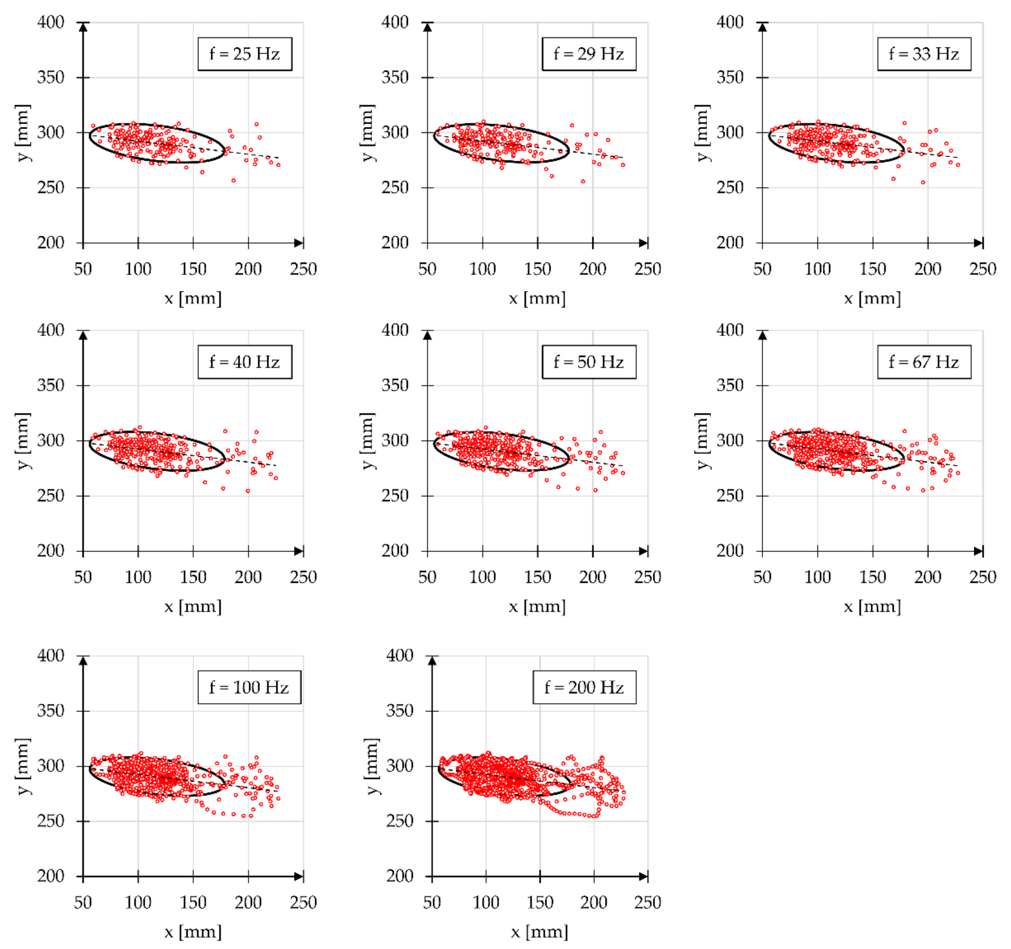
| f | n | a | b | α | xCOG | yCOG | ΔP | k | A |
|---|---|---|---|---|---|---|---|---|---|
| Hz | - | mm | mm | ° | mm | mm | - | % | mm2 |
| 25 | 230 | 61.46 | 16.00 | −6.80 | 117.35 | 290.60 | 0.58 | 83.9 | 3066.19 |
| 29 | 263 | 61.41 | 15.74 | −6.75 | 117.34 | 290.63 | 0.58 | 83.3 | 2874.56 |
| 33 | 306 | 61.43 | 16.05 | −6.75 | 117.30 | 290.62 | 0.58 | 84.0 | 3066.19 |
| 40 | 367 | 61.46 | 16.09 | −6.78 | 117.29 | 290.56 | 0.57 | 84.5 | 3066.19 |
| 50 | 459 | 61.40 | 15.86 | −6.81 | 117.28 | 290.58 | 0.57 | 84.3 | 2874.56 |
| 67 | 612 | 61.39 | 15.86 | −6.83 | 117.27 | 290.56 | 0.58 | 84.0 | 2874.56 |
| 100 | 918 | 61.37 | 15.84 | −6.84 | 117.26 | 290.56 | 0,58 | 84,5 | 2874,56 |
| 200 | 1835 | 61.37 | 15.83 | −6.84 | 117.24 | 290.55 | 0.61 | 84.1 | 2874.56 |
| μ | - | 61.41 | 15.86 | −6.80 | 117.29 | 290.58 | 0.58 | 84.08 | 2946.42 |
| σ | - | 0.04 | 0.08 | 0.04 | 0.04 | 0.03 | 0.01 | 0.39 | 99.18 |
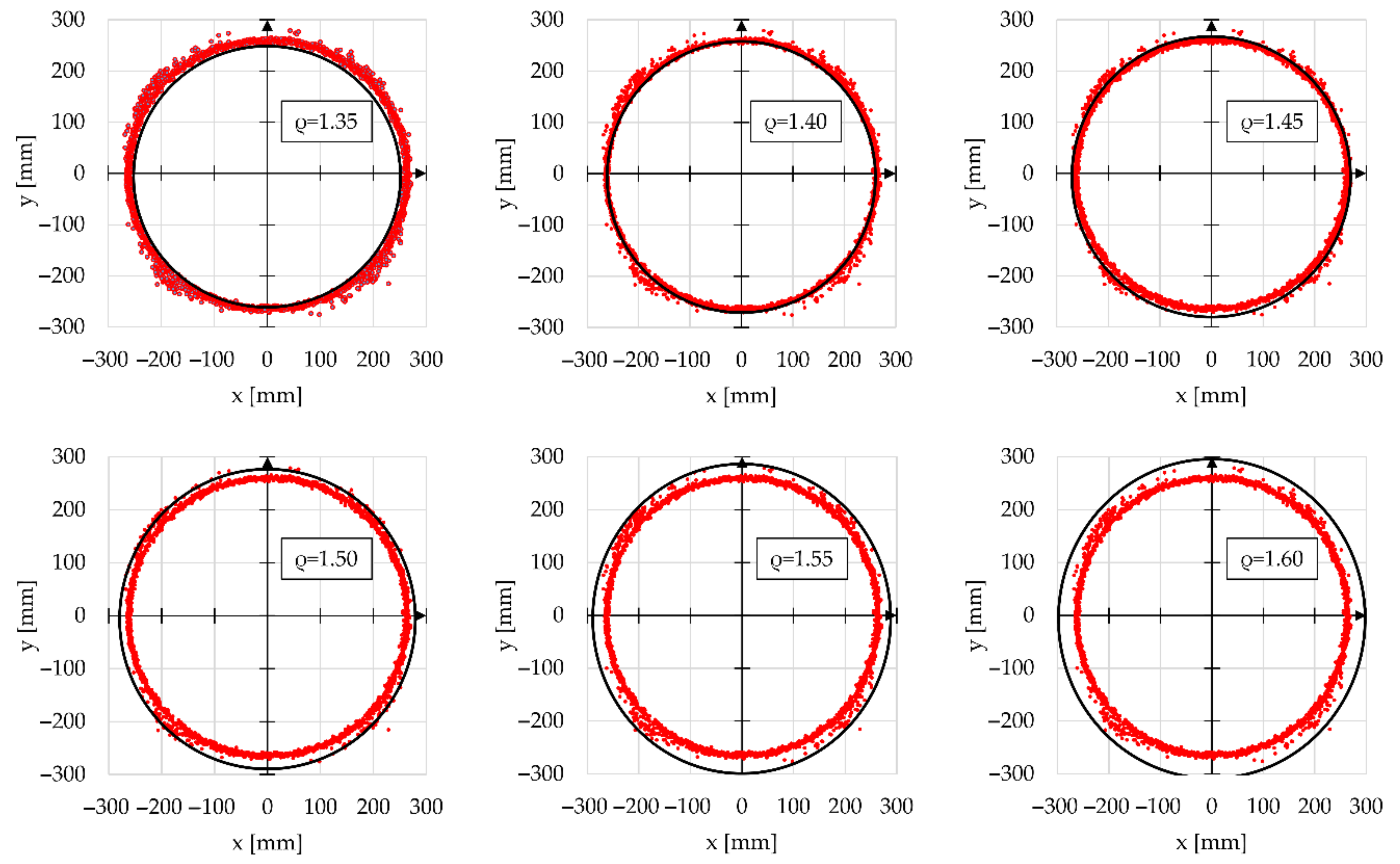
| ρ | a | b | α | xCOG | yCOG | ΔP | k | ΔR |
|---|---|---|---|---|---|---|---|---|
| - | mm | mm | ° | mm | mm | - | % | mm |
| 1.35 | 251.37 | 254.89 | −0.28 | −0.45 | −6.39 | 0.64 | 0.2 | 6.87 |
| 1.4 | 260.67 | 264.33 | −0.28 | −0.45 | −6.39 | 0.64 | 33.5 | 2.50 |
| 1.45 | 269.99 | 273.77 | −0.28 | −0.45 | −6.39 | 0.64 | 89.8 | 11.88 |
| 1.5 | 279.30 | 283.21 | −0.28 | −0.45 | −6.39 | 0.64 | 96.8 | 21.26 |
| 1.55 | 288.61 | 291.65 | −0.28 | −0.45 | −6.39 | 0.64 | 99.9 | 30.13 |
| 1.6 | 297.92 | 302.09 | −0.28 | −0.45 | −6.39 | 0.64 | 100.0 | 40.01 |
| μ | 279.30 | 283.01 | - | - | - | - | - | 17.46 |
| σ | 14.72 | 14.77 | - | - | - | - | - | 16.48 |
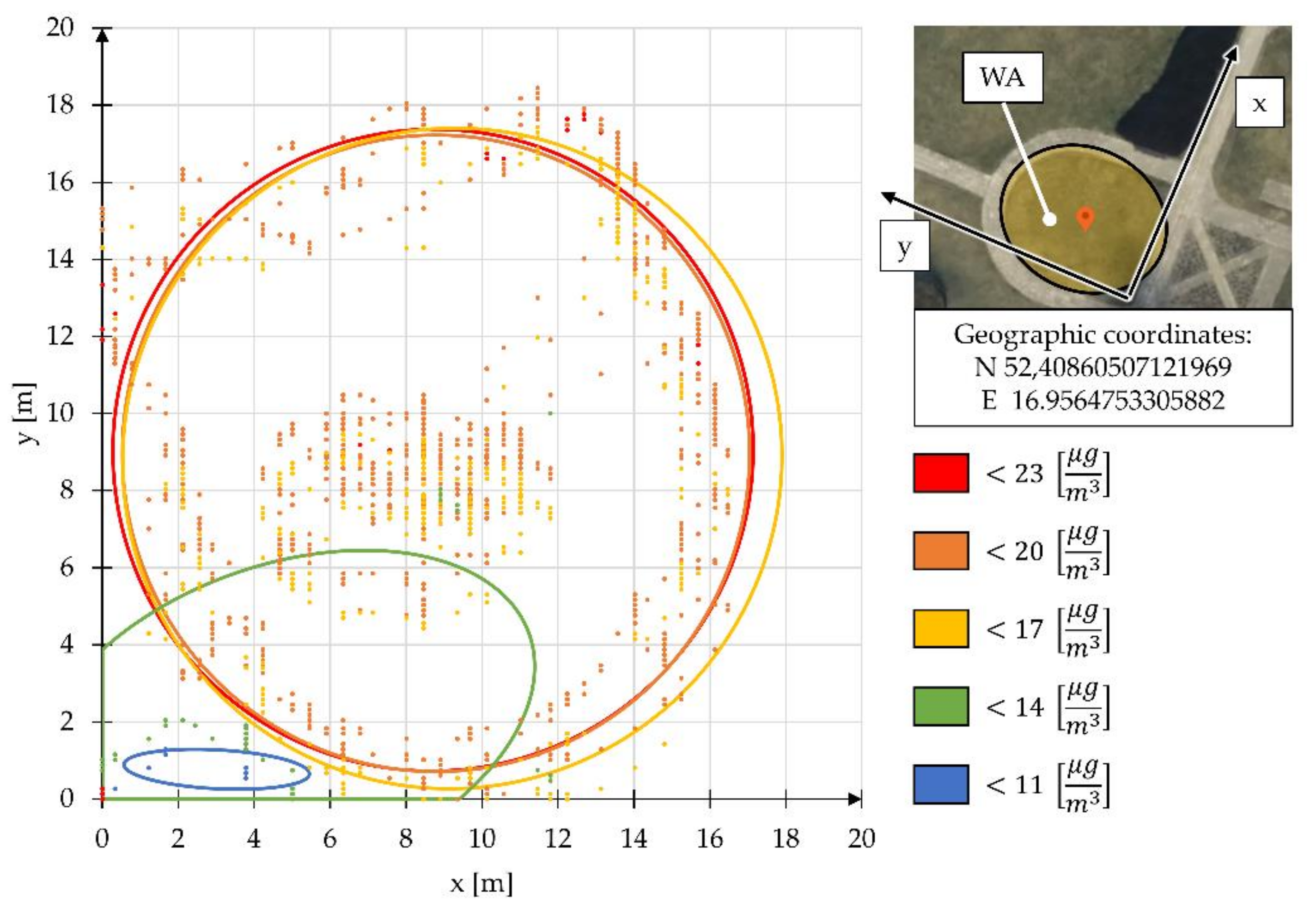
| PM 2.5 | a | b | α | xCOG | yCOG | ΔP | k | A |
|---|---|---|---|---|---|---|---|---|
| μg/m3 | m | m | ° | m | m | - | % | m |
| <23 | 8.43 | 8.33 | 7.90 | 8.71 | 9.05 | 0.61 | 82.7 | 220.50 |
| <20 | 8.26 | 8.26 | 6.17 | 8.79 | 8.97 | 0.58 | 82.6 | 214.21 |
| <17 | 8.69 | 8.55 | 18.00 | 9.21 | 8.83 | 0.59 | 88.2 | 233.63 |
| <14 | 6.84 | 4.05 | 19.10 | 4.79 | 2.01 | 0.79 | 79.3 | 87.10 |
| <11 | 2.44 | 0.50 | −2.94 | 3.01 | 0.77 | 0.31 | 87.5 | 3.87 |
| μ | 6.56 | 3.83 | 10.47 | 6.45 | 5.15 | 0.57 | 84.4 | 134.70 |
| σ | 2.86 | 3.83 | 10.47 | 3.04 | 4.37 | 0.20 | 4.2 | 108.77 |
Publisher’s Note: MDPI stays neutral with regard to jurisdictional claims in published maps and institutional affiliations. |
© 2022 by the authors. Licensee MDPI, Basel, Switzerland. This article is an open access article distributed under the terms and conditions of the Creative Commons Attribution (CC BY) license (https://creativecommons.org/licenses/by/4.0/).
Share and Cite
Wieczorek, B.; Kukla, M.; Warguła, Ł. Describing a Set of Points with Elliptical Areas: Mathematical Description and Verification on Operational Tests of Technical Devices. Appl. Sci. 2022, 12, 445. https://doi.org/10.3390/app12010445
Wieczorek B, Kukla M, Warguła Ł. Describing a Set of Points with Elliptical Areas: Mathematical Description and Verification on Operational Tests of Technical Devices. Applied Sciences. 2022; 12(1):445. https://doi.org/10.3390/app12010445
Chicago/Turabian StyleWieczorek, Bartosz, Mateusz Kukla, and Łukasz Warguła. 2022. "Describing a Set of Points with Elliptical Areas: Mathematical Description and Verification on Operational Tests of Technical Devices" Applied Sciences 12, no. 1: 445. https://doi.org/10.3390/app12010445
APA StyleWieczorek, B., Kukla, M., & Warguła, Ł. (2022). Describing a Set of Points with Elliptical Areas: Mathematical Description and Verification on Operational Tests of Technical Devices. Applied Sciences, 12(1), 445. https://doi.org/10.3390/app12010445