Estimation of Acoustic Source Positioning Error Determined by One-Dimensional Linear Location Technique

Abstract

The one-dimensional (1D) linear location technique has been considered as one of the methods for determining the position of acoustic emission (AE) sources in metallic objects. However, this approach does not take into account the heterogeneity of materials and that leads to poor accuracy of AE sources localization. To estimate the positioning error of the linear location technique which is typically used to determine the AE source location a new approach based on the combination of experimental and simulation methods is proposed. This approach for error estimation contains a finite element model construction of the AE signals localization. The model consists of transmitting and receiving transducers mounted on the test object, the frequency response of which selected close to the characteristics of acoustic emission transducers applied in the preliminary experiments. The application of the approach in current research showed that a reduced positioning error on a flat steel plate reaches 15%. The proposed technique can be used to optimize the number of preliminary tests required to calculate the reduced error of the 1D linear location technique applied for the AE sources localization during the inspection of the structure.

1. Introduction

Acoustic Emission (AE) is one of the most efficient techniques which enables the determination of any faults and structural issues prematurely. The physical phenomena of AE monitoring are based on the elastic waves (ultrasonic signals) generation caused by the processes of defects initiation and propagation in materials [1]. This high-sensitivity method makes it possible to assess the accumulation degree of developing internal defects in materials with different physical and mechanical properties, for example, in composites [2], concrete structures [3], rocks [4] and metals [5].

To identify defects in structures using the AE method, the following stages should be carried out. Loading the structure and recording AE signals are done simultaneously at the beginning of AE diagnostics. During load tests, defects generate acoustic signals and further analysis of them reveals the defects’ presence and their parameters. Moreover, the risk assessment of defect occurrence also can be performed. Thus, to capture data of AE sources, the energy and spectral characteristics of the recorded AE signals [6] are analyzed. It should be noted that they can differ significantly depending on the type of loading [7] and the metals’ structure [8]. In addition, the reliability of risk assessment of internal defects largely depends on the accuracy of AE sources localization which is carried out by means of processing recorded AE signals. Therefore, one of the main tasks of structural AE monitoring is to determine the coordinates (location) of acoustic signal sources, namely defects. Ththe focus of this paper is to improve the efficiency of AE source coordinates determination in isotropic metal products.

Generally, the transition of elastic energy released by internal damages can be measured by the group of piezoelectric transducers (receiving AE sensors) bonded to the surface of an object under study. When the time difference of arrival (TDOA) u_th is registered by each AE sensor and wave velocity V_g of acoustic signals is calculated, the emission source position can be obtained [9]. As a rule, the acoustic wave velocity in the media is estimated in accordance with the standardized Hsu–Nielsen test (breaking the lead of a pencil with a diameter of 0.3 mm). However, the standard algorithm for measuring wave velocity V_g can fail to meet the accuracy requirement due to the great attenuation of high-frequency modes of the spectrum of the acoustic signal in the tested material. As a result, there is a significant effect on the shape of the recorded AE signals and the parameter Δt. Moreover, the accuracy of the AE sources localization determined by the conventional method using the threshold approach mostly depends on the fixed thresholding level for the acoustic signals u_th and bandwidth of digital filters Δf. Additionally, it should be mentioned that these characteristics can cause a considerable effect on the acoustic wave velocity parameter.

To reduce the influence of the dispersion properties of the acoustic channel on the determination of AE source location coordinates, the “Δt-mapping” algorithm [10,11,12] can be applied. It includes the recording of Δt values during preliminary tests. Implementation of the “Δt -mapping” location algorithm allows detecting AE sources coordinates without using the V_g parameter.

In this paper, the positioning error of the linear location technique which is typically used to determine the AE source location [13] has been assessed in reliance on the combination of both experimental and simulation results.

The developed approach for the error estimation contains a FE model construction of the AE signals localization. The generation and registration of acoustic signals using piezoelectric AETs are simulated. Referring to [5], the spectrum of the recorded AE signals is the product of the amplitude-frequency characteristics (AFC) of the acoustic path, the AE source, and the receiving transducer. To build a reliable finite element model of the localization process of AE signals, it is necessary to determine each of the above frequency characteristics. The frequency response of the acoustic signal source can be represented as a broadband spectrum in the frequency range used for recording AE signals. The frequency characteristics of the receiving transducers can be modeled based on the information given in the equipment passport. The most difficult task is to determine the frequency response of the acoustic path since its solution requires numerous preliminary tests to assess the characteristics of propagation, attenuation, and conversion of the main modes of the recorded AE signals.

Taking into account the combined effect of the frequency characteristics of the AETs and the acoustic path when constructing a finite element model, it is proposed to transform the receiving transducer models so that the shape of their frequency characteristics correlates with the spectrum of the recorded AE signals. The model development is carried out according to the results of preliminary experimental studies. The experimental part consists of imitating acoustic signals on the surface of the test object using a broadband transducer. Preliminary experimental tests are needed due to the lack of a priori information on the influence of the frequency characteristics of the receiving transducers and the acoustic path on the spectrum of the recorded AE signals.

Based on the experimental data captured during the implementation of the 1D linear location technique of AE sources on a steel plate, a finite element model of the transmitting and receiving transducers is developed. This makes it possible to create a computer simulation of AE signals propagation in the acoustic path of the test object; to determine the average level of the reduced error of the 1D linear location technique depending on the position of the receiving AETs in relation to the AE transmitter, and to define the amplitude level of the recorded acoustic signals.

The development of an analytical model describing the propagation of AE signals in the test object allows reducing the number of preliminary tests required to assess the reduced error of the 1D linear location technique when identifying structural damages [14,15,16,17].

2. Experimental Method and Results

The approach proposed in this paper to assess the reduced error of the linear location technique of AE sources was implemented using a steel plate as the simplest isotropic object for control. The methodology of computational and experimental studies consisted of the following stages.

At the initial stage, a series of laboratory experiments (Section 2) was carried out to estimate the accuracy of the 1D linear location technique. An electronic simulator was installed on the surface of a steel sample. It was applied to imitate an AE source presence. Based on the results of experimental studies, the reduced error of the 1D linear location technique was calculated. The shapes and spectra of the AE signals were also recorded.

Then, a finite element model was developed (Section 3) to simulate the generation and registration processes of acoustic signals by AETs. To increase the reliability of the FE model, the frequency characteristics of the modeled AE signals correlated with spectra parameters of AE signals were recorded experimentally. The developed AET models were used to assess the reduced error of the 1D linear location technique of AE sources by means of modeling.

The efficiency of this approach was confirmed by comparing experimental and modeling calculations of the reduced error, as well as by the correlation assessment of the obtained dependences (Section 4).

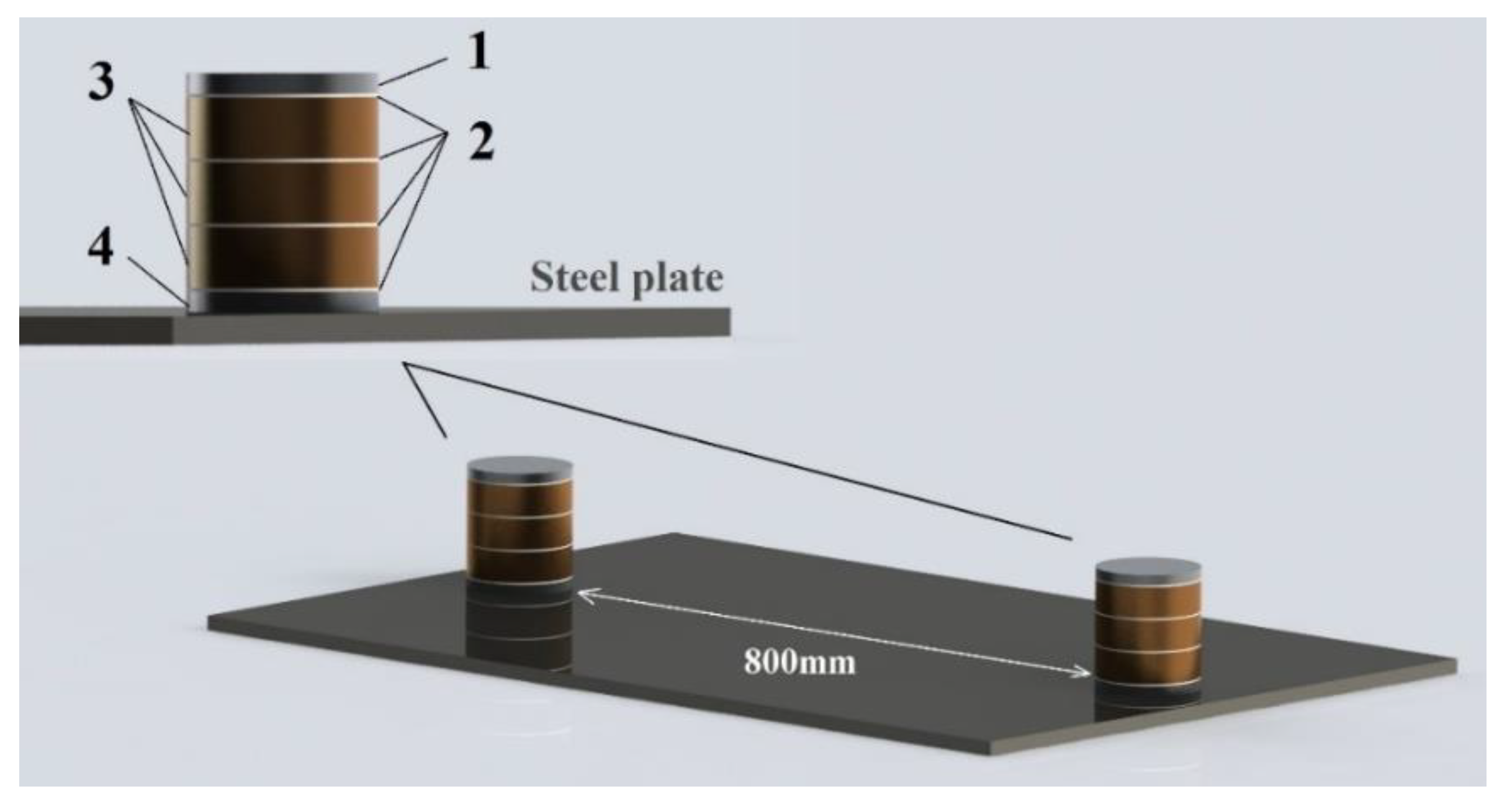
2.1. Methods and Materials

Several experiments were carried out to study the 1D linear location method. In the beginning, AE events were generated by the INTERUNIS-IT electronic simulator equipped with a UT-1000 broadband transmitting transducer. The experiments were performed on a steel plate with dimensions of 1000 × 650 × 7 mm presented in Figure 1.

Registration of AE events and detection of their source location was performed using two receiving transducers “VS150-RIC” with a preamplifier connected to the system “Vallen AMSY-6”. Those receiving transducers (AE sensors #1 and #2) were located on the surface of the steel plate with an 800 mm distance between them (B = 800 mm). The transmitting transducer was installed on the surface as well, but its coordinates were changed for each experiment X = 100, 200, … 700 mm in respect to the AE sensor #1.

Before the experiments began, the parameters of measurement devices and the average wave velocity of AE signals V_g have been established. The standard methodology of AE monitoring is described in PB (Safety Rules) 03-593-03 «The guidelines for acoustic emission monitoring of vessels, apparatus, boilers and pipelines» and in ASTM E 976–99. The thresholding level u_th in the current research has been calculated by the equation:

u_th ≥ u_n + 6,

(1)

where u_n—maximum noise amplitude, dB.

Thus, the thresholding level equaled to u_th = 40 dB. The frequency bandwidth constituted Δf = 50–850 kHz. The wave velocity V_g was evaluated based on the pencil-lead-break experiment with acoustic signal generation. The pencil lead was broken outside the area between AE sensors #1 and #2 at a distance of 100 mm from AE sensor #1. The AE wave velocity in the steel plate was V_g = 4250 m/s with the distance between acoustic sensors B = 800 mm.

The amplitude of generated AE signals varied from 55 to 100 dB due to the potential difference of the AE simulator in the voltage range of 10–300 V. The process of acoustic source imitation consisted of alternately generating 250 AE signals in each of the coordinates X = 100, 200, … 700 mm. The calculation of the positioning error (γ) of the AE transmitting transducer was carried out by the equation [18]:

$$\gamma =\frac{\left|X_{real}-X\right|}{B}·100\%,$$

(2)

X_real—installation coordinate of the AE simulator, X—experimentally calculated coordinate of the AE simulator, B—the distance between AE sensors #1 and #2.

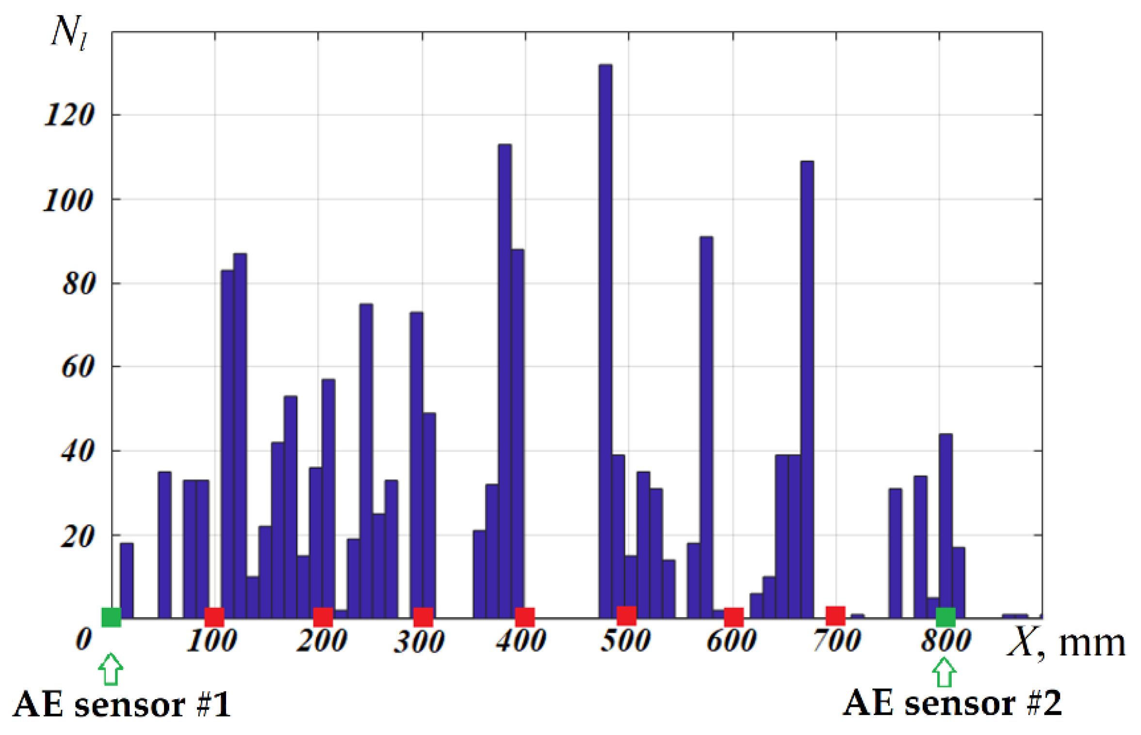
2.2. Experimental Results of Determining the AE Source Location on the Steel Plate

In Figure 2, the results of 1D linear location technique implementation with the UT-1000 transmitting transducer connected to the INTERUNIS-IT acoustic simulator were presented. The histogram of the AE source location pattern was figured with the coordinate axis discretization step of 10 mm.

As can be seen from Figure 2, the transmitting transducer positions on the steel plate were highlighted by red color, while the fixed locations of the receiving transducers were marked as the green one. The dark blue columns displayed the distribution of AE events N_l recorded at each position of the AE simulator (UT-1000) on the distance varied from 100 to 700 mm from the AE sensor #1. It follows from the column graph that the highest reduced error was noted when the acoustic source was located at the X = 100 mm coordinate.

When the AE simulator was mounted on the plate at a distance of less than 200 mm from AE sensor #1, it was impossible to clearly determine its position due to the scattering of AE signals. Since the distance between the AE source and the receiving transducers increased, the range of the calculated coordinates has tended to a noticeable decrease. Thus, the positioning error γ of the linear location technique did not exceed 2.5% in the coordinates X = 400 and 500 mm. The results of experimentally determined γ which is basically dependent on the acoustic source location and the amplitude of AE signals were given in

Table 1. The experimental results of the AE source positioning error.

Coordinates of AE Source X, mm	Amplitudes Interval of Recorded AE Signals [umin:umax], dB	Positioning Error γ, %	Average Positioning Error γav, %
100	[40:60]	14.9	8.6
	[60:75]	8.3
	[75:100]	2.5
200	[40:60]	10.4	5.8
	[60:75]	5.0
	[75:100]	1.9
300	[40:60]	7.2	4.4
	[60:75]	4.1
	[75:100]	1.9
400	[40:60]	2.5	2.1
	[60:75]	2.05
	[75:100]	1.8
500	[40:60]	2.4	2.2
	[60:75]	2.1
	[75:100]	2.0
600	[40:60]	7.6	5.4
	[60:75]	5.1
	[75:100]	3.6
700	[40:60]	13.4	8.6
	[60:75]	8.5
	[75:100]	3.9

.

From Table 1 it can be derived that the highest average error of the AE source location was registered when the acoustic simulator of low-amplitude signals located in the coordinate X = 100 mm. In case the acoustic source was mounted at the center between two receiving transducers, the location error equaled to γ_av ≈ 2%.

2.3. Experimental Results Discussion

The application of the thresholding approach for recording acoustic signals is one of the main reasons for the AE source positioning error growing determined by the 1D linear location method. Since higher frequencies were attenuated more rapidly with propagation distance, significant changes in the initial steepness of the AE signals envelope have been observed. This fact led to a considerable increase in the parameter Δt. In Figure 3, the waveforms and spectra of low-amplitude acoustic signals recorded by AE sensors at a distance of 100 mm and 700 mm from the acoustic source were presented, respectively.

The waveform registered–by AE sensor #1 was depicted in Figure 3a. It can be inferred that the maximum AE signal amplitude corresponded to the u_max = 56 dB, and the rise time equaled to t_n = 64 μs.

The spectrum of this signal was shown in Figure 3b, where three special frequency ranges can be distinguished: 40–160 kHz, 160–250 kHz, 250–400 kHz. With attenuation of high-frequency modes, the energy decreased and the slope of the AE signal envelope at the initial moment declined as well. It caused a significant effect on the value of the parameter Δt [19,20].

In Figure 3c the signal waveform registered by the further receiving transducer (AE sensor #2) was represented. Its maximum amplitude constituted u_max = 52 dB, and the rise time was about t_n = 102 μs. The growth in the rise time of the AE signal correlated with the fall in the partial energy of the spectrum in the frequency range 250–400 kHz. Thus, the rapid attenuation of high-frequency modes influenced the recording time of acoustic signals, and hence, on the level of the investigated positioning error. This fact was confirmed by the estimation of relative changes in the high-frequency portion of the spectrum δ revealed in Figure 4. The dependence of the attenuation of high-frequency spectral components on the AE signal propagation length L was evaluated according to the equation [14]:

$$\delta =\frac{\left|H{\left(f\right)}_1-H{\left(f\right)}_2\right|}{H{\left(f\right)}_1}, \left[\%\right]$$

(3)

where H(f)₁ and H(f)₂ cumulative amplitudes of AE signals harmonics registered by AE sensor #1 and AE sensor 2 in the range of 250–400 kHz. The approximation of the calculated results of the parameter δ was performed by the least-squares method fitting with a second-degree polynomial.

From the curve shown in Figure 4 and results from Table 1, it can be indicated that the considerable attenuation of high-frequency waves leads to a great change in the energy parameters and the signal waveform. Therefore, to determine the correct location of an AE source, it is essential to take into account not only the TDOA parameter of signals but also their energy and spectral characteristics [21].

3. FEM Analysis and Results

3.1. Methods and Materials

To make an estimation of the average location error of the linear location technique using the computational approach [22,23,24], an FE model of the receiving transducer was developed. Moreover, the frequency response of the modeled transducers was fully identical to the parameters of AE sensors used in the experiments.

Figure 5 depicts a finite element model of a typical acoustic emission transducer. The software “Comsol Multiphysics” was applied to prepare a FE model during this study.

A typical model of the AE sensor included an aluminum damper (1), three plates of a lead zirconate titanate piezoelectric element (3), four layers of epoxy resin (2) and a damping protector (4). The FE model was done in accordance with the boundary conditions and parameters of the electric circuit to create the inverse piezoelectric effect. The end faces of the test object were fixed to minimize repeated reflections of the acoustic waves from the side faces of the plate. The elastic displacements were assigned to the upper and lower surfaces of the steel plate. It allowed generating multimode AE signals. In addition to this, a grid of tetrahedral elements was applied, the facet size of which was 250 μm. An electrical signal of a rectangular form with an amplitude of 100–300 V was utilized as an exciting signal. In order to simulate Lamb waves in the object of the study, some restrictions were imposed on the displacement of the AE sensors in respect to their fixed place on the steel plate.

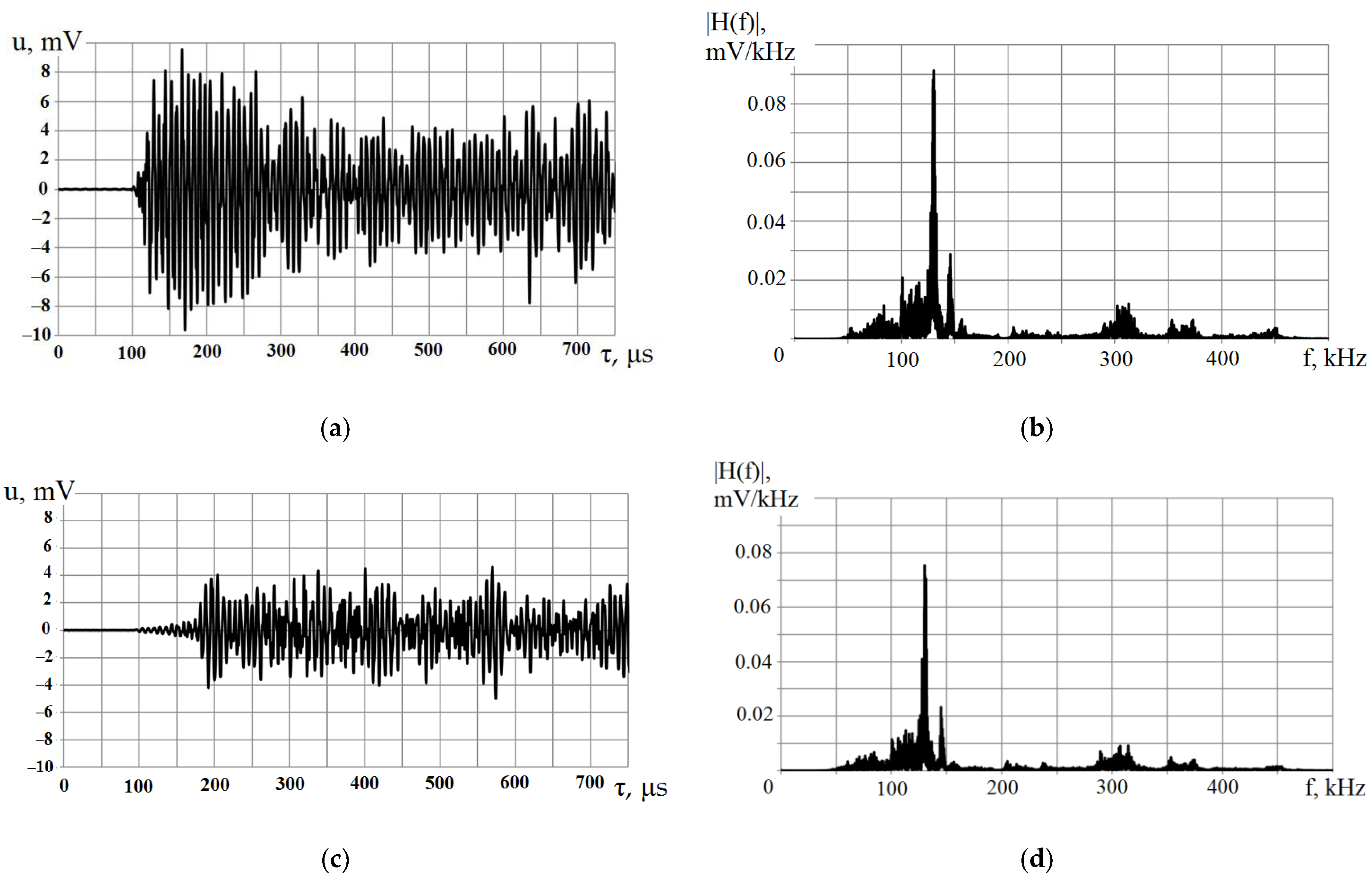
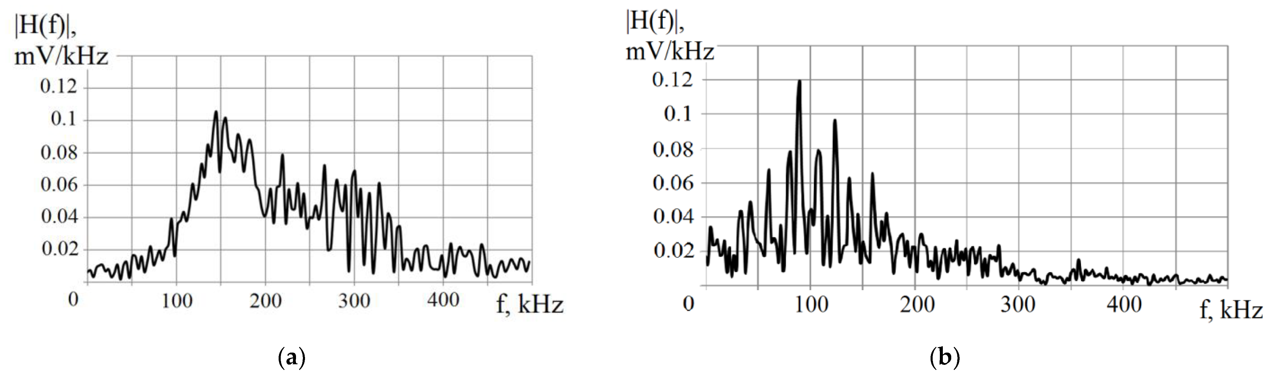
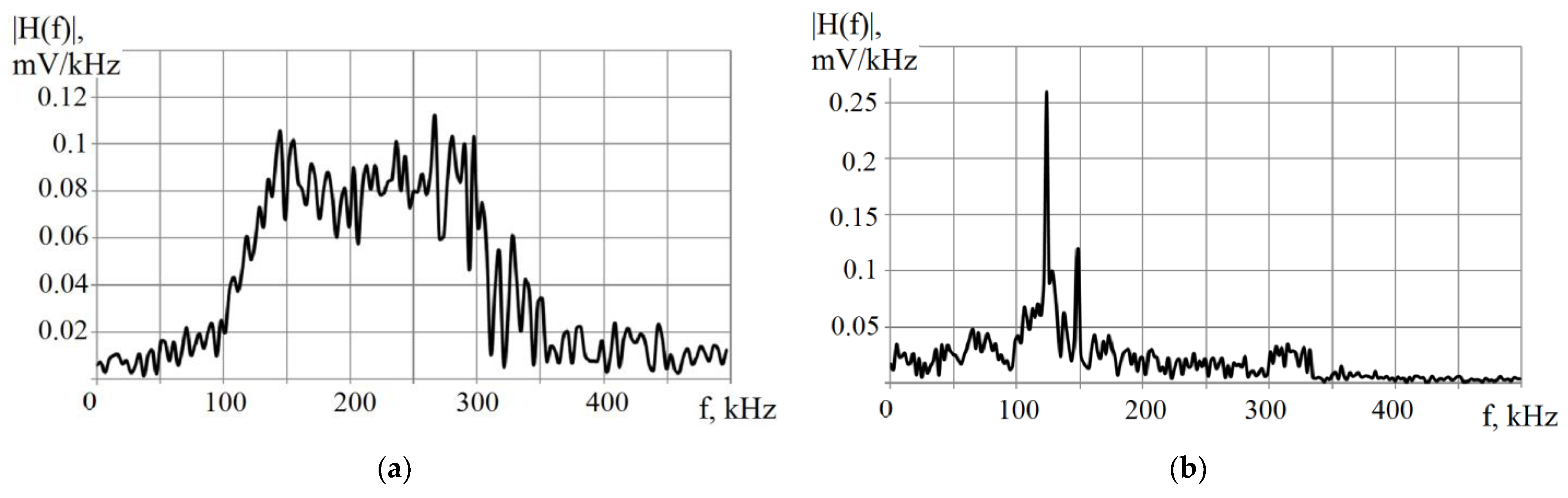
3.2. Finite-Element Model of AETs. Frequency Response Correspondence

The influence of transducer design on its frequency response was investigated by finite element modeling. It is widely known that the damper size and the number of piezoelectric elements can be considered as major design features that caused a significant effect on the transducer bandwidth. In Figure 6 the frequency response of transducers with a damper of various heights was shown.

The transducer with a piezoelectric element height of 3 mm, a damping protector of 1 mm and an upper damper with a thickness of 0.5 mm had the frequency response presented in Figure 6a. A decrease in the damper thickness resulted in an evident increase in the bandwidth of a receiving transducer up to 350 kHz. As shown in Figure 6b, growth in the thickness of the upper damper caused low sensitivity of the transducer in the frequency range above 200 kHz, as well as a decline in the resonance frequency from 150 to 80 kHz.

Comparison of the obtained numerical models of transducers included one and five piezoplates was carried out. The studied effect of increasing the number of piezoelectric plates on the transducer bandwidth was inferred in Figure 7.

From the frequency response of the transducer model with one piezoelectric element, 1 mm damping protector and an upper protector height of 3 mm, the local maximum of the energy density distribution at frequencies of 160 and 340 kHz can be noticed. The greater the number of piezoelectric elements, the more perceptible equalization of the energy density distribution in the 80–200 kHz passband will be. Based on the simulation results, the optimal design features of the AE source and receiving transducers (AE sensors) were selected for FEM analysis of acoustic signal propagation in a steel plate model. The model of the AE source included four piezoelectric plates 3 mm thick, a damping protector 1 mm thick, and an upper damper 0.5 mm thick, while the model of AE sensors consisted of two piezoelectric plates 3 mm thick, a damping protector 1 mm thick, and an upper damper 4 mm thick. Their frequency response graphs were shown in Figure 8.

The AE source of broadband acoustic signals had the frequency response given in Figure 8a. Four piezoelectric elements made it possible to expand the passband of the acoustic signal source up to 120–300 kHz. In Figure 8b the frequency response of the receiving transducer model was displayed. The optimal FE model of the AE transducer obtained the same spectral characteristics as the AE sensors from the experimental part had, see Figure 3. To numerically estimate the similarity of the recorded AE signals spectra (Figure 3b) and the frequency response of the receiving transducer FE model, the correlation coefficient r was computed:

$$r=\frac{\overline{\left|H{\left(f\right)}_1·H{\left(f\right)}_2\right|}-\overline{\left|H{\left(f\right)}_1\right|}·\overline{\left|H{\left(f\right)}_2\right|}}{{\sigma }_1·{\sigma }_2}$$

(4)

where H(f)₁ and σ₁—the average value and dispersion of the spectral characteristics of the recorded AE signals; H(f)₂ and σ₂—the average value and dispersion of the spectral characteristics of the receiving transducer model.

The correlation coefficient value between the results shown in Figure 3b and Figure 8b was r = 0.82.

3.3. Simulation Approach to Detect the AE Source Location

The simulation of the AE signals propagation in a steel plate was carried out in accordance with the experimental scheme (see Figure 1). The optimal design of AE sensors and the acoustic source was implemented to simulate broadband signals, the spectral characteristics of which were close to the VS150-RIC transducers used in experiments with a steel plate.

At the initial stage, the dependence of the calculated coordinate X on the amplitude of the recorded signals u_m was investigated using a linear location technique. As an example, the dependence of the calculated coordinate on the amplitude of the simulated signals X(u_m) when X = 100, 200, and 300 mm is graphically represented in Figure 9.

As follows from the scatter plots in Figure 9, the largest variability of X values was established when the AE source was located at a distance of X = 100 mm from AE sensor #1. The minimum error of the AE source location was noted when the signal amplitude constituted at least 80 dB. It was defined without reference to the AE simulator distance to the AE sensor #1. When the AE source was removed at X = 300 mm, an increase in the positioning error was indicated for signals with a maximum amplitude level of u_m ≤ 52 dB. It is also worth mentioning that the scatter of the X coordinate values is associated with the threshold discrimination of the AE signals oscillating shape. The latter ones have been recorded in the framework of modeling the propagation process of elastic waves in the isotropic metal plate.

3.4. The Model Results of Linear Location Technique for AE Source Positioning

The average positioning error was calculated for the 1D linear location method with the varied location of the AE source. Figure 10 showed the results of the AE sources linear location coordinates obtained by FE-modeling. The histogram of the location pattern was performed by discretizing the coordinate axis with a step of 10 mm.

It can be seen from Figure 10 that the largest scatter ΔX was defined when the AE source was located at X = 100 and 700 mm. Therefore, when the acoustic emission source got closer to the AE sensor, the ΔX achieved 200 mm. With the AE source moving away from the AE sensors, the difference between the calculated coordinates significantly decreased and did not exceed ΔX = 30 mm. Thus, in the coordinates X = 400 and 500 mm, the value of the location error was less than 5%. Moreover, it even reached γ_av = 2% in the center of the studied area. The highest value of location error was observed when AE sources located at 100 mm from one of the AE sensor γ_av = 8.6%.

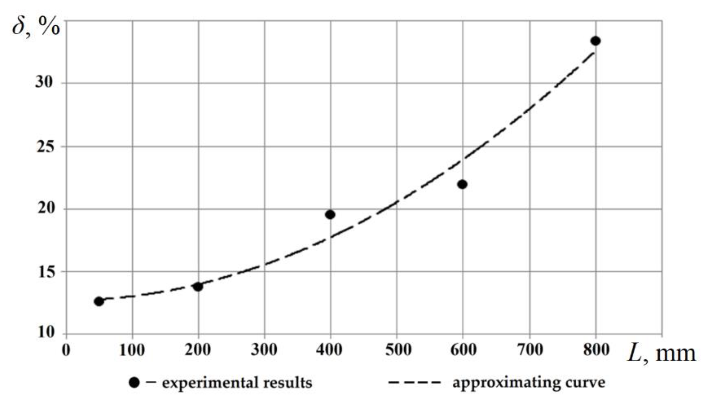
4. Comparison of the AE Source Positioning Error Obtained by the Experimental and Simulation Studies

The comparison between the average location error of AE source determined by experimental and computational approaches was graphically represented in Figure 11. The dashed line presents the interpolation of finite element modeling results by the least-squares method fitting with a third-degree polynomial.

It can be inferred from Figure 11 that the maximum level of the location error was registered in the coordinates X = 100 and 700 mm. Application of FEM analysis allowed to estimate with high accuracy the level of the average location error and at the same time avoid carrying out a large number of preliminary tests. The high precision of the calculation was confirmed by the correlation coefficient R = 0.92.

To minimize the positioning error, it is necessary to take into account not only the recording time of acoustic signals but also fluctuations in the wave velocity of AE signals. This approach can help to reduce the influence of the threshold algorithm on the values of ∆t. For the numerical calculation of V_g fluctuations, statistical models of multiple linear regression and machine learning methods can be used.

5. Conclusions

• The influence of the acoustic dispersion on the reduced error of AE source location has been considered. AE monitoring was performed using a thresholding approach. The location error calculated at a distance of less than 100 mm from the AE transducer reached 15% in respect to the whole investigated area;
• Finite element modeling of AE signals allowed to estimate with high accuracy the positioning error of the linear location technique applied to determine the AE source coordinates;
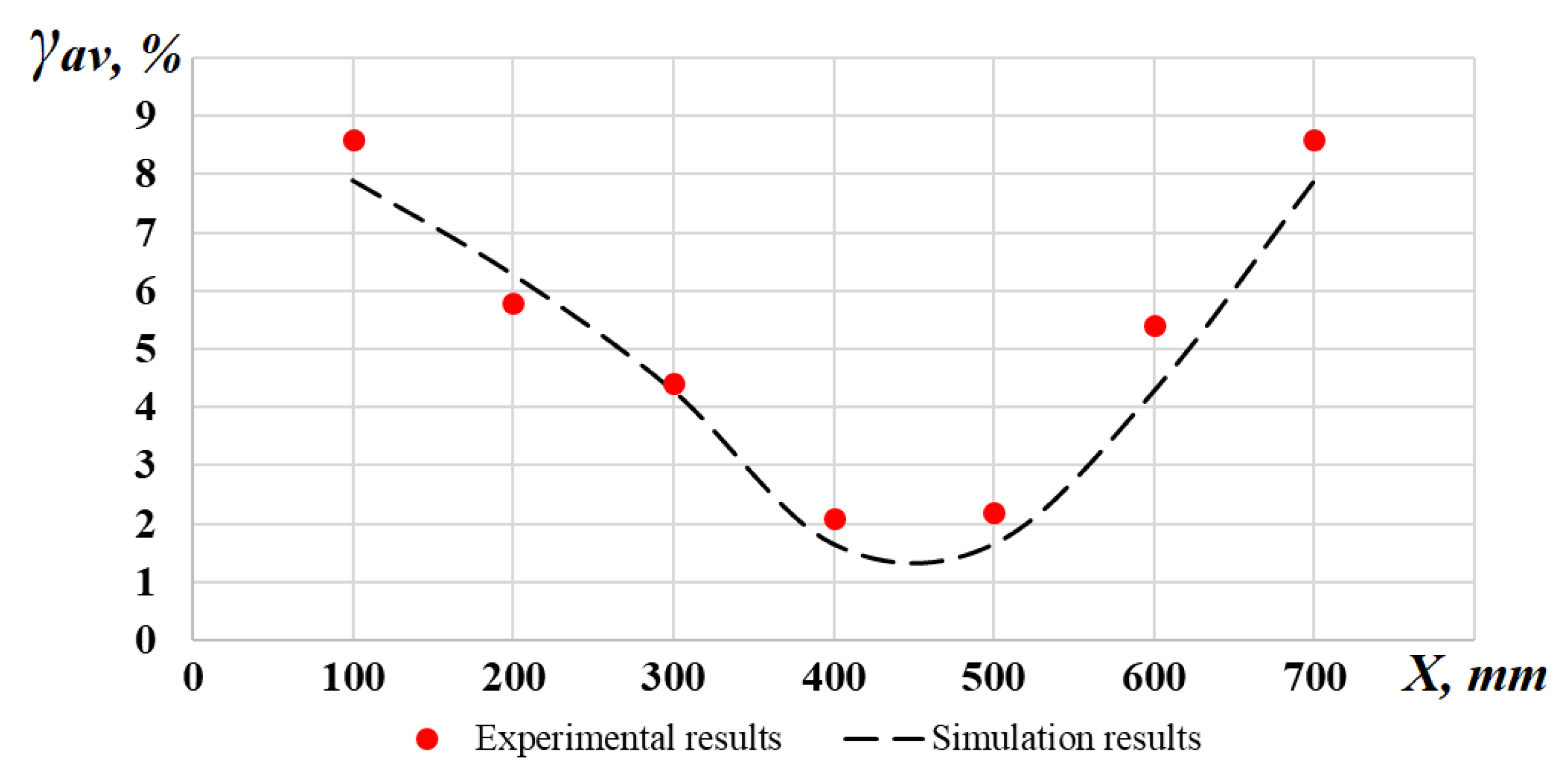
• The experimentally obtained data corresponded to the simulation results (see Figure 11). It implies that the developed FE model of acoustic wave propagation in a steel plate can be implemented to determine the AE source location with the required level of accuracy. Moreover, only a few preliminary tests should be carried out for a model construction;
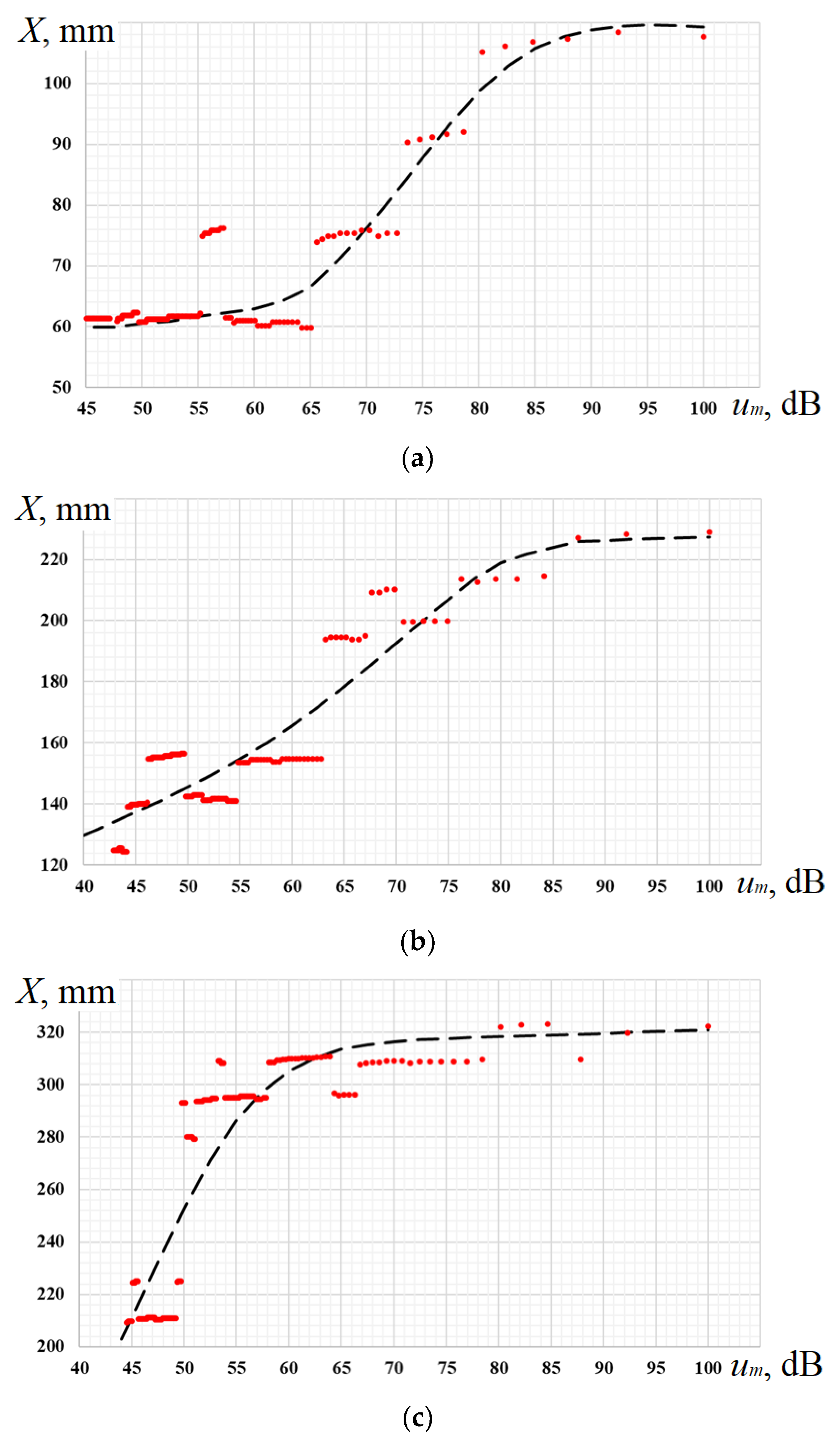
• The optimization method for assessing the reduced error of the 1D linear location technique of AE sources consists of several stages. At the initial stage, it is necessary to generate acoustic signals of various amplitudes using an electronic simulator. Then it is alternately installed at a distance of 0.1 B and 0.3 B (B—distance between two AETs) relative to one of the receiving transducers. Based on the results of the two experiments, there is a need to evaluate the spectral characteristics of the recorded AE signals, as well as to construct FE models of receiving AEs. Finally, a comparison between the error obtained by simulation and the results of preliminary tests should be done.
• The obtained results can be effectively used in the framework of acoustic emission monitoring of isotropic metal structures. There are many more potential applications offering benefits to the diagnostics adopting this approach. Especially it concerns maintenance inspections of extended objects with complex geometry.

References

1. Grosse, C.U.; Ohtsu, M. Acoustic Emission Testing, Basics for Research; Applications in Civil Engineering, Springer: Leipzig, Germany, 2008; p. 414. [Google Scholar]
2. Matvienko, Y.G.; Vasil’ev, I.E.; Chernov, D.V.; Ivanov, V.I.; Mishchenko, I.V. Error reduction in determining the wave-packet speed in composite materials. Instrum. Exp. Tech. 2020, 63, 106–111. [Google Scholar] [CrossRef]
3. Mpalaskas, A.C.; Matikas, T.E.; Aggelis, D.G.; Alver, N. Acoustic Emission for Evaluating the Reinforcement Effectiveness in Steel Fiber Reinforced Concrete. Appl. Sci. 2021, 11, 3850. [Google Scholar] [CrossRef]
4. Dixon, N.; Smith, A.; Flint, J.A.; Khanna, R.; Clark, B.; Andjelkovic, M. An acoustic emission landslide early warning system for communities in low-income and middle-income countries. Landslides 2018, 15, 1631–1644. [Google Scholar] [CrossRef] [Green Version]
5. Zou, S.; Yan, F.; Yang, G.; Sun, W. The Identification of the Deformation Stage of a Metal Specimen Based on Acoustic Emission Data Analysis. Sensors 2017, 17, 789. [Google Scholar] [CrossRef] [Green Version]
6. Vinogradov, A.; Danyuk, A.; Merson, D.; Yasnikov, I. Probing elementary dislocation mechanisms of local plastic deformation by the advanced acoustic emission technique. Scr. Mater. 2018, 151, 53–56. [Google Scholar] [CrossRef] [Green Version]
7. Louda, P.; Sharko, A.; Stepanchikov, D. An Acoustic Emission Method for Assessing the Degree of Degradation of Mechanical Properties and Residual Life of Metal Structures under Complex Dynamic Deformation Stresses. Materials 2021, 14, 2090. [Google Scholar] [CrossRef]
8. Ma, W.; Luo, H.; Han, Z.; Zhang, L.; Yang, X. The Influence of Different Microstructure on Tensile Deformation and Acoustic Emission Behaviors of Low-Alloy Steel. Materials 2020, 13, 4981. [Google Scholar] [CrossRef]
9. Zhou, Z.-L.; Zhou, J.; Dong, L.-J.; Cai, X.; Rui, Y.-C.; Ke, C.-T. Experimental study on the location of an acoustic emission source considering refraction in different media. Sci. Rep. 2017, 7, 7472. [Google Scholar] [CrossRef] [Green Version]
10. Baxter, M.; Pullin, R.; Holford, K.; Evans, S. Delta T source location for acoustic emission. Mech. Syst. Signal Processing 2007, 21, 1512–1520. [Google Scholar] [CrossRef]
11. Al-Jumaili, S.; Pearson, M.; Holford, K.; Eaton, M.; Pullin, R. Acoustic emission source location in complex structures using full automatic delta T mapping technique. Mech. Syst. Signal Processing 2016, 72–73, 513–524. [Google Scholar] [CrossRef]
12. Pullin, R.; Baxter, M.; Eaton, M.; Holford, K.; Evans, S. Novel acoustic emission source detection. J. Acoust. Emiss. 2007, 25, 215–223. [Google Scholar]
13. Stepanova, L.N.; Kabanov, S.I.; Ramazanov, I.S.; Kanifadin, K.V. Analysis of errors in location of flaws in multipass welds using different clustering methods. Russ. J. Nondestruct. Test. 2017, 53, 96–103. [Google Scholar] [CrossRef]
14. Chernyaeva, E.V.; Volkov, A.E.; Galkin, D.I.; Bigus, G.A.; Merson, D.L.; Bystrova, N.A. Evaluation of the condition of a metal using the acoustic-emission method: Prospects and problems. Russ. J. Nondestruct. Test. 2013, 49, 131–139. [Google Scholar] [CrossRef]
15. Tang, J.; Wang, Y.; Li, J.; Wang, H.; Chen, G. In-situ monitoring and analysis of the pitting corrosion of carbon steel by acoustic emission. Appl. Sci. 2019, 9, 706. [Google Scholar] [CrossRef] [Green Version]
16. Terentyev, D.A.; Popkov, Y.S. Determination of the parameters of the dispersion curves of Lamb waves with the use of the Hough transform of the spectrogram of an AE signal. Russ. J. Nondestruct. Test. 2014, 50, 19–28. [Google Scholar] [CrossRef]
17. Lukonge, A.; Cao, X. Leak detection system for long-distance onshore and offshore gas pipeline using acoustic emission technology. A review. Trans. Indian Inst. Met. 2020, 73, 1715–1727. [Google Scholar] [CrossRef]
18. Raghavendra, N.V. Engineering Metrology and Measurements; OUP India: New Delhi, India, 2013; p. 546. [Google Scholar]
19. Skal’s’kyi, V.R.; Pochaps’kyi, E.P.; Klym, B.P.; Rudak, M.O.; Velykyi, P.P. Application of the method of magnetoelastic acoustic emission for the analysis of the technical state of 19g steel after long-term operation in an oil pipeline. Mater. Sci. 2016, 52, 385–389. [Google Scholar] [CrossRef]
20. Matvienko, Y.G.; Vasiliev, I.E.; Chernov, D.V.; Marchenkov, A.Y. Diagnostics of welded joints in main pipelines equipment. Sci. Technol. Oil Oil Prod. Pipeline Transp. 2018, 8, 618–630. [Google Scholar] [CrossRef]
21. Makhutov, N.A.; Vasil’iev, I.E.; Chernov, D.V.; Ivanov, V.I.; Elizarov, S.V. Influence of the passband of frequency filters on the parameters of acoustic emission pulses. Russ. J. Nondestruct. Test. 2019, 55, 173–180. [Google Scholar] [CrossRef]
22. Gerasimov, S.I.; Sych, T.V. Finite element modeling of acoustic emission sensors. J. Phys. Conf. Ser. 2017, 881, 012003. [Google Scholar] [CrossRef] [Green Version]
23. Junior, C.A.P.; Nascimento, V.H.; Lopes, C.G. Modeling time of arrival probability distribution and TDOA bias in acoustic emission testing. In Proceedings of the 2018 26th European Signal Processing Conference (EUSIPCO), Rome, Italy, 3–7 September 2018; pp. 1122–1126. [Google Scholar]
24. Sause, M.G.R.; Richer, S. Finite Element Modelling of Cracks as Acoustic Emission Sources. J. Nondestruct. Eval. 2015, 34, 4–17. [Google Scholar] [CrossRef] [Green Version]
Figure 1. Scheme of experimental determination of AE source location on the steel plate.
Applsci 12 00224 g001
Figure 2. Experimental result of AE source linear location recorded on a steel plate. —AE source location; —AE sensors location, X—coordinate, Nl—number of recorded AE events (responses from the AE source).
Applsci 12 00224 g002
Figure 3. Comparison of the signal waveforms and spectra recorded by (a,b) AE sensor #1 and (c,d) AE sensor #2 located at a distance of 100 mm and 700 mm from the AE source, respectively.
Applsci 12 00224 g003
Figure 4. Dependence of the relative attenuation δ of high-frequency spectral components on the distance L between the AE sensors and AE source.
Applsci 12 00224 g004
Figure 5. Typical model of an AE sensor: (1)—damper, (2)—bonding layer, (3)—piezoelectric element, (4)—damping protector.
Applsci 12 00224 g005
Figure 6. The frequency response of transducers with a damper thickness of (a) 0.5 mm and (b) 5 mm.
Applsci 12 00224 g006
Figure 7. The frequency response of transducers with (a) one and (b) five piezoelectric elements.
Applsci 12 00224 g007
Figure 8. The frequency response of (a) AE source and (b) AE sensor.
Applsci 12 00224 g008
Figure 9. The dependence of the calculated coordinate X on the amplitude um of the simulated signals at the distance between the AE source and AE sensor #1 (a) 100 mm, (b) 200 mm and (c) 300 mm.
Applsci 12 00224 g009
Figure 10. Simulation results of AE source coordinate determination. —AE source location; —AE sensors location; Nl—the number of AE events.
Applsci 12 00224 g010
Figure 11. Comparison of the average location error for experimental and computational methods.
Applsci 12 00224 g011