Analyzing Multiscale Spatial Relationships between the House Price and Visual Environment Factors

Abstract

House price is closely associated with the development of the national economy and people’s daily life. Understanding the spatial distribution characteristics and influencing factors of the house price is of great practical significance. Although a lot of attention has been paid to modeling the house price from structure and location attributes, limited work has considered the impact of visual attributes. Intuitively, a better visual environment may raise the surrounding house price. When aggregating multiple factors that influence house price, the multiscale geographically weighted regression (MGWR) provides a suitable solution. Specifically, the MGWR assigns each factor a bandwidth to model the spatial heterogeneity, e.g., a factor may have different influences at different places. In this paper, we introduce the visual environment factors into the MGWR method. In detail, we extract ten visual elements, e.g., sky, vegetation, road, from the Baidu street view (BSV) images, using a deep learning framework. We further define six visual environment factors to investigate their influence on house price. Based on the data from two representative Chinese cities, i.e., Beijing and Chongqing, we reveal the influence degree and spatial scale difference of six visual indexes on the house price in two cities. Results show that: (1) the influence intensity of our proposed six visual environment factors on the house price in different regions of the city can be identified, and the green view index (GVI) is the most important visual environmental factor; and (2) the influence of these view indexes changes significantly or even reversely depends on different areas.

1. Introduction

As a hot topic concerning the government, real estate investors, and residents, the house price is strongly associated with economic activities and people’s daily life. Investigating the spatial distribution characteristics and influencing factors of the house price can provide suggestions for house buyers, as well as researchers in the real estate market. Exploring the influencing factors of house prices has always been a research hotspot, and many relevant references have made achievements in this regard. In these studies, the decisive factors of house price are diverse and complex, which are generally classified into three categories: structure attributes, location attributes, and physical environment attributes.

First, structure attributes refer to the properties of the house, such as the number of bedrooms, area, and age. T.H.Tan et al. [1] find that the number of bedrooms and private space is important influencing factors for first-time buyers. When exploring the relationship between house orientation and house price in Shanghai, Lu et al. [2] proved that the house prices in residential areas facing south are higher because they can enjoy more sunshine and beautiful scenery facing south. The floor is also one of the important factors affecting the house price. Xiao et al. [3] believe that the comfort of the landscape, in the same building on different floors, has vertical heterogeneity. Because the landscape viewing of different floors is different, the floor will also affect the house price. In Saudi Arabia, the size of the kitchen and the number of bedrooms are the most important factors influencing the house price [4]. Second, location attributes mainly refer to the accessibility of the house to the surrounding infrastructure (such as transportation facilities, education facilities). People are also willing to pay extra for houses closer to schools and subway stations. Residential areas with transfer stations in the suburbs also have higher house prices than residential areas without transfer stations [5,6]. Educational facilities are another influencing factor widely concerning everyone. Families with children are more willing to buy houses near the school at a higher price to ensure that children get better educational resources [7]. The quality of school education also significantly promotes the surrounding house prices. Wen et al. [8] take Hangzhou as an example and find that the quality of secondary education has the most significant impact on house prices, followed by primary schools and high school education. Last, physical environment attributes mainly refer to the urban landscape, such as rivers, mountains, and parks. The urban landscape provides aesthetic, entertainment, and ecological functions, which are beneficial to the spiritual, emotional, and physical health of residents. In China, with the improvement of the quality of life, people have begun to pursue a higher quality of living environment. In Hangzhou, mountains, lakes, rivers, parks, and other internal urban landscapes have a positive impact on house prices [9,10]. Through questionnaire surveys and field research, some studies have shown that street visual appearance not only directly affects residents’ impression but also affects the house price of the neighborhoods [11,12]. The emergence of big data and map services provides unprecedented opportunities to obtain a new kind of geographic data—street view images. As a kind of idiographic data, the street view images can be adopted to represent the local scenes of neighborhoods while emphasizing human perception [13,14]. Although studies have shown that the sky view factor and building height affect the house price [15], the impact of other visual factors on the house price has not been confirmed. There are still few studies that explore the relationship between visual environment elements and house prices.

Spatial heterogeneity is another common phenomenon in geographic distribution. At present, many references at home and abroad generally confirm the spatial heterogeneity of some house price-influencing factors. Existing house price methods, such as the hedonic price model (HPM) proposed by Rosen, typically only explore the relationships between influencing factors and the house price on a global scale, ignoring the spatial heterogeneity of influencing factors [16]. Kang et al. [17] introduced the GWR to model the spatial relationships between influencing factors and house price appreciation. Although classic GWR can solve part of the spatial heterogeneity problem, which cannot be handled by traditional linear regression models, it ignores the scale problem of spatial heterogeneity of different influencing factors and causes large estimation errors [18,19,20]. Goodchild [21] claimed, “scale is perhaps the most important topic of geographical information science”. However, there is little research on the scale difference of spatial heterogeneity of different house price-influencing factors. When explaining a certain socioeconomic phenomenon, the understanding of the "spatial scale effect" is very important. MGWR was proposed by Fotheringham by allowing the bandwidths of each variable to be different, thereby obtaining more credible estimation results and giving the scale of influence of different variables. Recently, MGWR has been introduced to examine the spatial variation of researchers in China [22] and explore the spatially nonstationary relationships between variables and COVID-19 incidence rates [23]. However, there are few studies on MGWR modeling the house price-influencing factors.

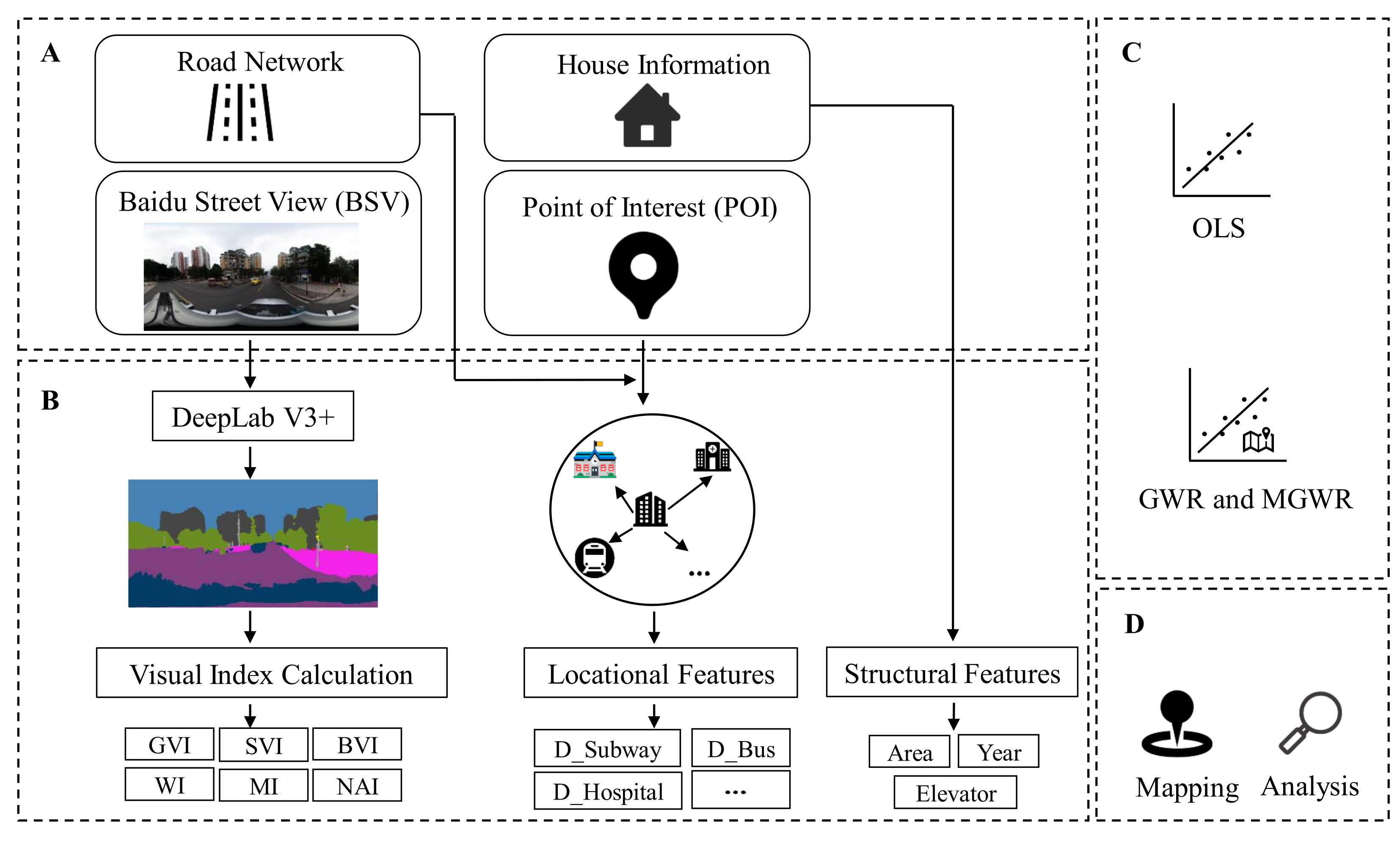
To sum up, quantifying the physical environment and exploring the influence of visual environment factors on house prices is of practical significance. Due to the spatial heterogeneity of influencing factors, using the geospatial model to understand the spatial relationship between influencing factors and house prices are necessary. In this work, we analyze the visual environment factors of house prices by considering multiscale effects. Compared with the traditional house price models, such as HPM and GWR, the MGWR can not only effectively deal with spatial heterogeneity of house price but can also identify the exclusive bandwidths for each influencing factor. The bandwidth can reflect the ranges of operational scales between influencing factors and house prices. First, ten visual elements of BSV images are extracted based on the deep learning methods, and six visual indexes affecting the house price are defined. Second, MGWR is introduced to explore the spatial heterogeneity relationships between six visual indexes and the house price. Last, the estimation accuracy of HPM, GWR, and MGWR are compared. Extensive experiments are conducted in Beijing and Chongqing, and results show that: (1) the influence intensity of six visual indexes on the house price in different regions of the city can be identified, while the same visual factors have different effects on different neighborhoods due to the combination differences of structure attributes and location attributes. The house prices in Beijing and Chongqing are very sensitive to visual factors, and there is a high degree of spatial heterogeneity. The scale of the GVI is the largest of all visual variables and is close to a global scale; (2) the R-squared and interpretation ability of MGWR are higher than HPM and GWR. The results of this study can provide a scientific basis and theoretical guidance for urban facilities planning and community street environment design in different cities.

2. Framework

2.1. Overview

The framework is composed of four stages, namely data collection, feature extraction, model construction, and mapping and analysis (Figure 1). First, we collect multi-source datasets, including the road network, house information, BSV images, and point of interest (POI). Second, by fusing the above datasets, we extract a series of features that are assumed to have an impact on the house price. Then, MGWR is built using the features constructed. Finally, we interpret the potential variables that are associated with the house price.

2.2. Data Collection

Four different categories of data are used in this study, namely road network, house information, BSV images, and POI, as shown in

Table 1. Datasets of the study area.

Datasets	Description	Data Source
House prices	Including area, date, total prices	Lianjia
POIs	Including name, type, location	Amap
Road networks	Road, community boundaries	Open Street Map
BSV images	Baidu Street View images	Baidu Maps

.

• House price data. House price data comes from a popular online real estate website—Homelink—which mainly describes the structural attributes of houses. Each record of house prices includes the location, area, unit price, etc. A total of 20,785 records in Beijing were obtained after processing and 20,098 records in Chongqing were obtained after processing.
• POI data. Typically, locational amenities refer to the facilities near the house. Here, we use the POI information to show the location characteristics of a nearby house. POI data were collected from Amap, which consists of nine subcategories: primary schools, parks, subway stations, etc. Finally, 13,532 POI records were obtained in Beijing and 8918 POI records in Chongqing.
• Road network data. The road network data was downloaded from the Open Street Map (OSM). After extracting five types of roads, including highways, primary, secondary roads, tertiary roads, and residential roads, 4412 roads within the fifth ring road of Beijing and 2137 roads in the main urban area of Chongqing were obtained. Combined with the distribution of the neighborhood and the connectivity of the road network, the study area was divided into 1640 research units and 747 research units, respectively.
• BSV images data. BSV images are downloaded by utilizing the Baidu street view API. BSV images have been widely used to describe the physical settings of urban environments and neighborhoods. A set of geo-referenced sampling points are generated along the roads with a fixed distance interval of 50 m. Finally, 64,569 panorama images in Beijing were collected after removing pictures of indoor or abnormal through visual inspection, and 38,987 images were obtained in Chongqing. The time and volume at which the data sources were collected have been listed in

  Table 2. Time and volume of the data sources.

  Datasets	Collecting Time	Volume
  		Beijing	Chongqing
  House prices	May 2021	20,785 records	20,098 records
  POIs	July 2021	13,532 records	8918 records
  Road networks	July 2021	4412 edges	2137 edges
  BSV images	September 2019	64,569 images	38,987 images

  .

2.3. Feature Extraction

2.3.1. Street Visual Features

Excepting these hard factors, the soft factors, such as visual characteristics of a community, which reflect the safety, lively, depressing, or beauty of the neighborhood environment, also have an impact on the house price [24,25,26]. The DeepLab V3+ [27,28] deep learning framework was adopted for the semantic segmentation and extracting of visual features from BSV images. Ten categories of visual elements, road, sidewalk, sky, building, vegetation, vehicle, person, traffic_sign, pole, and fence, were extracted from BSV images, as shown in Figure 2.

Based on the existing studies and related theories of house prices [29], this paper proposed six visual indices using the information extracted from the BSV images. The detailed computation method for each index is as follows.

• Green View Index (GVI), Building View Index (BVI), Sky View Index (SVI). Existing researches have proven that using street view images can explore the relationships between a set of visual elements and its social-economic attributes, such as the crime rate, the property value, and the population density, well [30,31]. Referring to the GVI calculation formula proposed by [32,33,34], the calculation formulas of BVI and SVI are proposed, respectively.

  $$GVI=\frac{P_v}{P_t}$$

  (1)

  $$SVI=\frac{P_s}{P_t}$$

  (2)

  $$BVI=\frac{P_b}{P_t}$$

  (3)
  $P_v$, $P_s$, and $P_b$ refer to the number of vegetation, sky, and building pixels in a panorama, and $P_t$ refers to the number of total pixels in a panorama. The higher the GVI value is, the more vegetation there is. The BVI reflects the height and continuity of the buildings on both sides of the street. SVI represents the area of sky elements from the perspective of human eyes, and the larger the SVI value indicates that the street vision is more open.
• Walkability Index (WI). The WI reflects the overall support of the outdoor context for walking. To focus on pedestrian feelings toward the streetscape from the perspective of perception, the WI is simplified as the extent of the visual impact of the horizontal perception environment [35,36,37]. WI is defined as follows:

  $$WI=\frac{\left(P_{si}+P_f\right)}{P_r}$$

  (4)
  $P_{si}$, $P_f$, and $P_r$ represent the number of sidewalk, fence, and road pixels in a panorama.
• Motorization Index (MI). The MI can describe the characteristics and properties of road traffic. H. Yue et al. have proven that MI has an impact on social and economic activities, reflecting the convenience of the community environment to a certain extent [38,39,40,41]. The MI calculation formula is defined as Equation (5).

  $$MI=\frac{\left(P_{si}+P_r+P_{ve}\right)}{P_t}$$

  (5)
  $P_{ve}$ represents the number of vehicle pixels in a panorama.
• Nature Artificial Index (NAI). With the improvement of living conditions, people have higher spiritual pursuits, and the basic hardware facilities can no longer meet people’s needs. Studies have shown that people are more willing to pay above the house price for communities with more natural environmental elements. NAI is defined as the percentage of the total pixels of natural elements in the total pixels of artificial elements in a panorama.

  $$NAI=\frac{P_n}{P_a}$$

  (6)
  $P_n$ refers to the number of natural elements pixels in a panorama; natural elements include vegetation and sky. $P_a$ refers to the number of artificial elements pixels in a panorama, and artificial elements include building, traffic_sign, fence, road, sidewalk, and pole.

2.3.2. Structural Features and Locational Features

Structural features are derived from the house information, and three categories are extracted: area, elevator, and the age of the house. For locational features, to better characterize the living convenience of neighborhoods thoroughly, we construct features from the distance from the house to the nearest facilities. In this paper, ArcGIS is used to construct the traffic network, and the network analysis method is used to measure the road length between the residential area and the urban facilities to obtain the real road distance between the residential area and the urban facilities [42,43]. Based on previous studies, eight location features are calculated in this paper [44]. The variable descriptive information is shown in

Table 3. Variables descriptive statistics.

Variables	Description	Beijing		Chongqing
		Mean	S.D.	Mean	S.D.
Locational features
D_Bus	Distance to the nearest bus station (km)	0.424	0.931	0.28	0.25
D_Subway	Distance to the nearest subway station (km)	1.457	1.565	0.953	0.672
D_Hospital	Distance to the nearest hospital (km)	0.913	1.255	0.919	0.756
D_Kindergarten	Distance to the nearest kindergarten (km)	0.778	0.698	0.313	0.325
D_PrimarySchool	Distance to the nearest primary school (km)	1.018	0.897	0.831	0.584
D_MiddleSchool	Distance to the nearest middle school (km)	1.287	1.167	1.157	0.735
D_Government	Distance to the nearest government (km)	0.646	1.062	0.271	0.3
D_Park	Distance to the nearest park (km)	1.564	1.515	0.965	0.653
Structural features
Elevator	Dummy variables (0 or 1)	0.485	0.499	0.504	0.499
Year	House age (year)	24.773	7.843	13.617	5.293
Area	Area (m${}^2$)	86.849	25.485	95.487	29.804
Visual features
GVI	Green View Index (%)	14.743	4.194	15.298	7.872
SVI	Sky View Index (%)	22.284	4.489	18.454	6.739
MI	Motorization Index (%)	23.075	2.56	27.332	3.561
WI	Walkability Index (%)	189.383	652.562	10.374	19.758
NAI	Nature Artificial Index (%)	2661.079	9976.847	2853.694	43,102.086
BVI	Building View Index (%)	3.309	1.192	5.021	2.895

.

2.4. Model Construction

2.4.1. Hedonic Price Model

The global regression is conducted by the hedonic price model (HPM). The HPM has three common forms: linear models, semilog models, and double-log models. In this study, the double-log form was adopted to build HPM because of the distribution of model variables. Based on the basic theory of the HPM, the double-log form HPM can explain the percentage change in the dependent variable caused by each unit of change in one dependent variable when the other independent variables are held constant. The HPM formula is given below.

$$ln\left(P_i\right)={\beta }_0+\sum _{j=1}^k{\beta }_j{x}_{ij}+\epsilon$$

(7)

In Formula (7), $P_i$ is the housing transaction price at the ith neighborhood unit, $ln\left(P_i\right)$ is the natural logarithm of $P_i$, ${\beta }_0$ is a constant, $x_{ij}$ is the jth independent variables for the ith neighborhood unit, ${\beta }_j$ is the corresponding estimated coefficient, and $\epsilon$ is an error term.

2.4.2. Multiscale Geographically Weighted Regression

Spatial nonstationarity is another common phenomenon in geographic distribution. However, the HPM neglects the spatial impacts of variables, and it cannot reveal the spatial dynamics of the relationship between spatial variables. The multiscale geographically weighted regression (MGWR) model can solve this problem. Therefore, we build the MGWR model to investigate the spatial nonstationarity and to investigate the influences on house prices. The MGWR model is an extended model of the GWR and semi-parametric geographically weighted regression (SGWR). Whereas both GWR and SGWR constrain the local relationships within each model to vary at the same spatial scale, MGWR allows the conditional relationships between the response variable and the different predictor variables to vary at different spatial scales. The calculation formula of MGWR is as follows:

$$ln\left(P_i\right)={\beta }_0\left(u_i,v_i\right)+\sum _{j=1}^k{\beta }_{bwj}\left(u_i,v_i\right)x_{ij}+{\epsilon }_i$$

(8)

where $\left(u_i,v_i\right)$ stand for the coordinates of the ith neighborhood unit, $bwj$ in ${\beta }_{bwj}$ indicates the bandwidth used for calibration of the jth conditional relationship, $x_{ij}{\beta }_{bwj}$ is the coefficient of the jth independent variables $x_{ij}$ at location $\left(u_i,v_i\right)$, and ${\epsilon }_i$ is the ith error term.

3. Experiment and Results

3.1. Spatial Distribution of the House Price

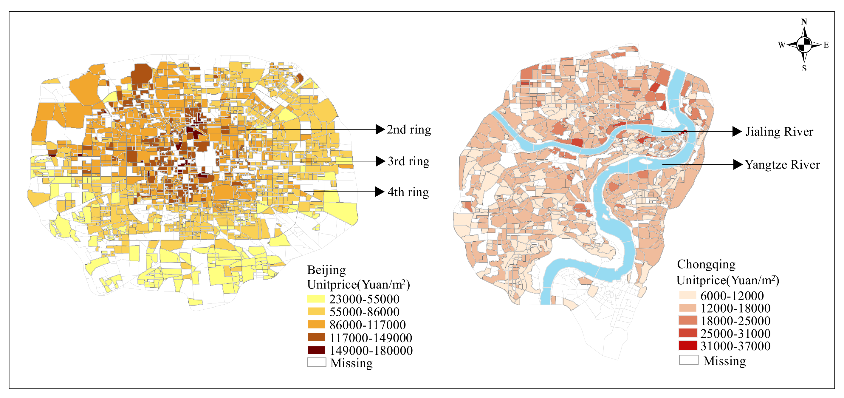
The weighted average method is adopted to aggregate the house price in the research unit in Beijing (Figure 3). Overall, the house price in Beijing fluctuates between 23,000 and 180,000 yuan within the fifth ring. Within the fourth ring region, the average house price is more than 55,000, the closer to the inner ring, the higher the house price. Outside the fourth ring road, the house price falls sharply. From the perspective of orientation, the house price is high in the northwest and low in the southeast. In most areas of Chongqing, the unit price fluctuates between 12,000 and 18,000 yuan. Divided by the river, the house price along both sides of the river are significantly higher than those in other regions. At the junction of the river, in the area near Chaotianmen, the house price fluctuates between 31,000 and 37,000, and the house price near Bashu Middle School in Yuzhong District is about 31,000. Due to the topography of Beijing, the difference between the development of the ring and the ring leads to the circular change of the house price, and there are high house price agglomeration distribution areas, while there is no high house price agglomeration distribution in Chongqing.

3.2. Spatial Distribution of Visual Indexes

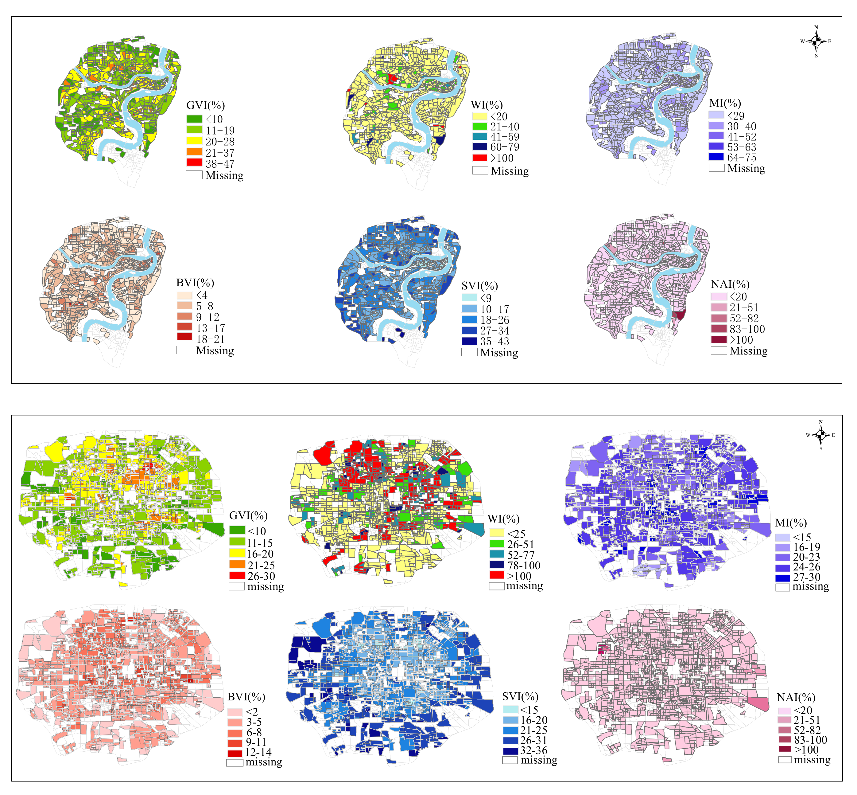
The weighted average method is adopted to aggregate visual indexes in the research units in Beijing and Chongqing. As shown in Figure 4, taking the GVI as an example, on the whole, the spatial distribution of the GVI is similar to that of the house price. The GVI is divided by the fourth Ring in Beijing. In the northwest, on both sides of Houhai and near Shichahai Park, the GVI value is higher than in other areas. In the southeast, the GVI value is higher in the area around Longtan Park. The GVI values near Loquat Mountain Park, Zourong Park, and Jialing Park in Chongqing were higher than those in other areas. Both cities showed that the GVI near the park was higher than other areas. The possible reason is that there is more vegetation and dense trees around the park, so the street view images captured more vegetation and accounted for more vegetation pixels.

3.3. Comparison of Models

Two metrics are used for the evaluation of model performance, namely, the corrected Akaike Information Criteria (AICc) and the coefficient of determination $R^2$. As can be seen from

Table 4. Comparison of models.

Model	Beijing		Chongqing
	${\mathit{R}}^2$	AICc	${\mathit{R}}^2$	AICc
HPM	0.56	3319.564	0.706	1221.922
GWR	0.834	2284.684	0.762	1168.135
MGWR	0.895	1815.088	0.831	1049.259

, the adjusted $R^2$ of the MGWR and GWR models is higher than that of HPM, and the AICc of the two models is lower than that of HPM. In addition, the adjusted $R^2$ of the MGWR model is higher than that of the GWR model, and the AICc is smaller than that of the GWR model. Therefore, in the process of Geospatial modeling, it is necessary to consider not only the spatial nonstationarity of the influencing factors but also the scale effect of different influencing factors on the dependent variables.

3.4. Spatial Scale Analysis

The bandwidths indicating the data-borrowing range can vary across parameter surfaces. The individual optimal bandwidths specific to each parameter in the MGWR model are given in

Table 5. Comparison of parameter bandwidth between MGWR and GWR.

Variables	Beijing		Chongqing
	MGWR	GWR	MGWR	GWR
Covariates
D_Bus	79	166	531	286
D_Subway	968	166	332	286
D_Hospital	1617	166	744	286
D_Kindergarten	1635	166	248	286
D_PrimarySchool	1518	166	97	286
D_MiddleSchool	127	166	736	286
D_Government	1214	166	744	286
D_Park	1336	166	744	286
Elevator	1635	166	218	286
Year	120	166	744	286
Area	43	166	44	286
Visual factors
GVI	1635	166	744	286
SVI	43	166	744	286
WI	43	166	733	286
MI	82	166	113	286
BVI	43	166	66	286
NAI	1635	166	240	286

, where it can be seen that the processes being modeled operate at different spatial scales. The GWR calibration yielded an optimal bandwidth of 166 nearest neighbors in Beijing, implying fairly localized processes. As can be seen from the table, the closer the bandwidth of the variable is to the total number of samples, the more likely it is to affect the house price on a large scale or even globally.

The parameter estimates associated with Beijing’s house price, such as the D_Hospital, the D_PrimarySchool, elevator, the GVI, and the NAI, are global; the optimal bandwidth in each case is as large as it could be (1640 nearest neighbors). The relationship between Beijing’s house price and the D_Subway exhibits spatial nonstationarity, but the process varies at a broad regional scale (optimal bandwidths of 968). The other variables have impacts on Beijing’s house prices that vary over relatively short distances, with the optimal bandwidths for the SVI being forty-three nearest neighbors, the MI being eighty-two nearest neighbors, and the BVI being forty-three nearest neighbors.

The parameter estimates associated with Chongqing’s house price, such as the D_hospital, the D_MiddleSchool, year, the GVI, and the SVI are global; the optimal bandwidth in each case is as large as it could be (747 nearest neighbors). The relationship between Chongqing’s house price and the D_Bus exhibits spatial nonstationarity, but the process varies at a broad regional scale (optimal bandwidths of 531). The other variables have impacts on Chongqing’s house price that vary over relatively short distances, with the optimal bandwidths for the area being forty-four nearest neighbors and the BVI being sixty-six nearest neighbors.

3.5. Results of the Global Regression Models

The HPM is used to model house prices by the visual factors selected in this paper and explore the global impact of visual factors on house prices. In this study, we controlled for a series of locational and structural variables, including D_Bus, D_Subway, D_Hospital, D_Kindergarten, D_PrimarySchool, D_MiddleSchool, D_Government, D_Park, Elevator, Year, and Area.

Table 6. Results of the global regression models.

Varibles	Beijing		Chongqing
	Coefficents	SE	Coefficents	SE
Covariates
D_Bus	−0.112 ***	0.019	−0.057 **	0.024
D_Subway	−0.120 ***	0.020	−0.131 ***	0.025
D_Hospital	0.050 ***	0.019	0.136 ***	0.026
D_Kindergarten	0.074	0.017	0.029	0.023
D_PrimarySchool	−0.037 **	0.018	0.027	0.024
D_MiddleSchool	−0.064 ***	0.018	−0.030 *	0.023
D_Government	0.038	0.018	0.051	0.024
D_Park	−0.096 ***	0.018	−0.036	0.022
Elevator	0.030 *	0.020	0.009 **	0.020
Year	−0.065 ***	0.017	−0.382 ***	0.025
Area	0.650 ***	0.017	0.770 ***	0.021
Visual factors
GVI	0.419 ***	0.067	0.218 ***	0.068
SVI	0.199 ***	0.070	0.241 **	0.062
WI	0.020	0.017	0.022	0.020
MI	0.072 ***	0.018	−0.040	0.028
BVI	−0.325 ***	0.035	−0.103 **	0.044
NAI	0.040 **	0.017	0.010 *	0.020

 * significant at the 0.1 level, ** significant at the 0.05 level, *** significant at the 0.01 level.

provides the OLS regression coefficient statistical description.

First, this paper selects eight influencing factors of location attributes. As can be seen from Table 4, factors affecting house prices in the global scope include six factors, the distance to the bus station, subway station, hospital, primary school, middle school, and park. In terms of transportation facilities and services, the distance between the bus station and subway station has a reverse promoting effect on housing prices. Specifically, the closer the distance between the bus station and subway station is, the higher the house price will be. According to the absolute value of the factor coefficient, the impact of the subway station on the housing price is greater than that of the bus station. In terms of health care, Chongqing and Beijing performed similarly, with housing prices falling the closer a neighborhood is to a hospital. Combined with the social functions of hospitals and the geomantic theory that Chinese people believe in, it is speculated that the complex noise and chaotic social environment of hospitals may make home buyers take extra consideration when buying houses. Therefore, hospitals near communities may restrain housing prices to some extent.

Second, from the perspective of structural attributes, the three structural characteristics of the two cities have a significant impact on the housing prices and have the same impact trend. Among them, the area and the presence of elevators have a positive impact on the housing price. That is to say, from the overall perspective, a house with an elevator has a larger area; therefore, the higher the price. Housing age refers to the difference between the current year and the year when the house was built. According to the regression coefficient, housing age is negatively correlated with housing price; that is, the house price of a new house is higher than that of an old house.

Last, it can be seen from Table 4 that the GVI, SVI, and BVI have the same influence trend on the house prices of the two cities. Specifically, the GVI and SVI are positively correlated with house prices; that is, the larger the GVI and SVI are, the higher house prices are. According to the literature review, street greening not only plays a role in the decoration of the city but also has a certain impact on the physical and mental health of urban residents. The more green vegetation visible on the street, the greater the proportion of visible sky, and the better walking experience for pedestrians. Therefore, the reasonable street design will improve the house prices of the community to a certain extent. The NAI has a positive correlation with the housing price of the two cities. According to the definition above, the NAI is the proportion of natural elements and artificial elements in a panorama. The more natural elements in the panorama, the higher the NAI. With the improvement of people’s quality of life, residents are more willing to spend more time with the natural environment, which not only adds vitality to the city but also brings visual comfort to the surrounding residents. Therefore, the natural environment of the community is also a factor affecting house prices.

In summary, in the covariates, the distance between transportation facilities, such as subway stations and bus stations, has a significant negative correlation with house prices in both cities, indicating that the closer to the subway station and bus station, the higher the house price. The distance between educational facilities, such as primary and secondary schools, has a significant negative correlation with urban house prices, indicating that the closer to the school, the higher the house prices. These two conclusions are consistent with the previous literature and our practice. Because the closer it is to the subway station and bus station, the more convenient it is for residents to travel, and the closer it is to the school, the better the educational resources. Among the structural attributes, the area is still the most critical factor affecting house prices. The larger the area, the higher the house prices. Among the visual elements, it is found that there is a significant negative correlation between the architectural visual index and house price in the two cities. It means that the larger the architectural visual index, the reverse promotion of house price growth. The possible reason is that the larger the architectural visual index, the denser and towering buildings, so it accounts for a large proportion of the street view. According to previous studies, dense buildings may bring people a greater sense of depression, which will directly affect residents’ walking experience and mental health.

3.6. MGWR Regression Coefficient Analysis

Similarly, we controlled for a series of locational and structural variables, adding visual factors to the MGWR model. The statistical description of the coefficients of the MGWR is shown in

Table 7. MGWR regression coefficient statistical description.

Variables	Beijing				Chongqing
	Mean	S.D.	Min	Max	Mean	S.D.	Min	Max
Covariates
D_Bus	−0.101	0.117	−0.556	−0.046	−0.065	0.022	−0.110	−0.037
D_Subway	−0.039	0.010	−0.061	−0.023	−0.091	0.042	−0.197	−0.048
D_Hospital	0.037	0.004	0.031	0.046	0.080	0.003	0.072	0.086
D_Kindergarten	0.026	0.003	0.020	0.033	0.013	0.028	−0.038	0.087
D_PrimarySchool	−0.022	0.010	−0.035	−0.006	−0.156	0.045	−0.263	−0.082
D_MiddleSchool	−0.024	0.073	−0.175	−0.045	−0.015	0.009	−0.028	−0.001
D_Government	0.041	0.015	0.021	0.063	0.035	0.008	0.024	0.047
D_Park	−0.053	0.091	−0.053	−0.019	−0.009	0.006	−0.020	−0.001
Elevator	0.008	0.002	0.005	0.014	0.208	0.453	0.113	1.571
Year	−0.035	0.054	−0.277	0.080	−0.406	0.162	−0.945	−0.103
Area	0.664	0.211	−0.042	1.305	0.717	0.147	0.331	1.308
Visual factors
GVI	0.299	0.003	0.295	0.304	0.161	0.004	0.168	0.156
SVI	0.185	0.204	−0.603	0.956	0.147	0.005	0.136	0.153
WI	−0.012	0.726	−1.775	2.245	0.004	0.004	−0.004	0.018
MI	0.033	0.109	−0.395	0.318	−0.068	0.084	−0.319	0.082
BVI	0.186	0.203	−0.450	0.924	−0.097	0.122	−0.608	0.222
NAI	0.196	1.473	0.038	3.910	0.599	1.016	0.390	2.918

. To see variations in the spatial scales at which the different processes operate more clearly, the weighted average method is adopted to aggregate coefficients of each variable in the research units in Beijing and Chongqing (as shown in Figure 5).

As shown in Table 7, six location variables significantly affect the house price in Beijing, namely, the D_Bus, D_Subway, D_Hospital, D_PrimarySchool, D_MiddleSchool, and D_Park. The coefficient of the D_Subway fluctuates between −0.061 and −0.032, indicating that as the distance to the subway decreases by 1 km, the house price of the northwest can rise by up to 0.061% in Beijing. The impact of traffic facilities on the house price in Chongqing is similar to that in Beijing. For every 1 km reduction in the distance to bus and subway in these areas, prices will rise by up to 0.110% and 0.197%. For structural attributes, in Chongqing, the area of houses is positively correlated with the house price on a global scope. Specifically, the house price increases by 0.717% on average for every 1 square meter increase in the house area. However, the area of houses has an opposite effect on the house price in different areas of Beijing.

The six visual indexes defined in this paper affect the house price to varying degrees. According to Figure 5, the GVI of the two cities both affect the house price on a global scope and are positively correlated with the house price. The average coefficients are 0.299 and 0.161, respectively. Specifically, when the GVI of Beijing and Chongqing increases by $1\%$, the house price increases by $0.299\%$ and $0.161\%$, respectively. The SVI is positively correlated with the urban house price; that is, the larger the SVI, the higher the house price. In Beijing, the SVI affects the house price on a local scope, among which the most influential areas are mainly in the Xidan North Street of the second ring Road and Shiji Jinyuan Shopping Center of the fourth ring road. While the SVI affects Chongqing’s house price on a global scope, the coefficient fluctuates between 0.136 and 0.153, the average coefficient is 0.147, indicating that with every $1\%$ increase of the SVI, the house price increases by $0.147\%$ on average. The MI affects the two cities’ house prices on a local scope, and the MI has the opposite effect on the house price in different regions. For example, near the People’s Square in Yuzhong District of Chongqing, the MI is negatively correlated with the house price. The D_PrimarySchool in this area also has a great impact on the house price, which may be the school district. Therefore, a large MI may not be friendly to the nearby schools. The influence of the MI on the house price in Beijing has a similar trend to that in Chongqing. Taking the western direction centered on Tian ’anmen Square and combining the distribution of the influence coefficient of the D_MiddleSchool, it is known that this area is mostly a middle school district, and the MI is negatively correlated with the house price. As can be seen from Figure 5, the impact of the BVI on the house price of the two cities is spatially nonstable. In particular, the BVI in the northwest of the third Ring in Beijing is negatively correlated with the house price, indicating that every $1\%$ reduction of the BVI will lead to a maximum $0.186\%$ increase in the house price. In the southwest of the third ring, the BVI is positively correlated with the house price. For Chongqing, the BVI has a significant negative correlation with the housing price; that is, the larger the BVI is, the lower the house price will be. High-rise and dense buildings may bring people a sense of psychological pressure, so the house price around them may be affected. The NAI mainly refers to the proportion between the sum of sky and green plants and other artificial environments. The NAI of the two cities is positively correlated with the house price. The more natural environmental elements near the residential area, the higher the house price of the residential area.

Based on the above analysis, the following conclusions can be obtained: (1) The GVI of the two cities has a significant impact on the house price. From the average coefficient, the GVI has a higher impact on the house price than other visual indexes. From the perspective of orientation, both cities show that the east, north, and south directions of the region’s house prices are the most affected. (2) According to Table 7 and Figure 5, the WI has the lowest impact on the house price. (3) There are spatial differences in the impact of all visual indexes on the house price; that is, the same street views visual index may have different effects on the house price in different regions to different degrees and trends. (4) The impact of the street visual environment index on the house price may be affected by other surrounding infrastructure. For example, near school districts, the MI has a negative correlation with the house price; that is, the smaller the MI, the higher the house price.

4. Conclusions

Among various factors that affect the house price, structure and location attributes have been intensively investigated. In this paper, we propose a new factor, the visual environment factor, for consideration. Our main contribution lies in that we extract ten visual elements and define six visual indexes to investigate their influences on house prices. To validate that our proposed indexes make sense, we introduce them into different methods, such as MGWR, GWR, and HPM. Then we implement our experiments on real-world data, which is extracted from Baidu Street View of Beijing and Chongqing. Some interesting results are as follows: (1) By visualizing the regression coefficient distribution, we can get the local or global change rules of different visual indexes affecting the house price. (2) The green view index is the most critical visual index affecting the house price and is positively correlated with the house price in the global scope. It indicates that the proportion of green area and vegetation in the community is positively promoting the rise of community house prices. Therefore, reasonable planning of community greening is not only conducive to the physical and mental health of residents but also conducive to the evaluation of house prices by real estate developers. (3) The sky view index, building view index, walkability index, motorization index, and nature artificial index also have a significant impact on the house price. Moreover, spatial heterogeneity exists in the influence of the five visual indexes on the house price, and the intensity of the visual indexes’ influence on the house price in different regions of the same city can be identified through the regression coefficient distribution. The influence intensity and trend of different visual indexes on house prices in different regions are significantly different. For example, near the school district, the motorization index has a significant negative correlation with house prices, while in the suburbs, the motorization index has a significant positive correlation with house prices. (4) In the MGWR, the influencing factors with small bandwidth have strong spatial heterogeneity and do not significantly affect the house price in the global scope. For example, the walkability index affects the house price only at small spatial scales. Our research integrates computer science and social science research by utilizing advanced techniques with emerging data sources and could provide new insights for buyers and urban planners.

In the future, we plan to improve this work in the following directions. First, we intend to incorporate the time attribute of BSV images into the relationship modeling of the house price and visual index and explore the influence of the physical environment on the house price in different stages with the change of time. Second, the influencing factors of the house price come from all aspects and are diverse; we plan to combine multi-source data (such as satellite remote sensing images) to enrich and quantify the factors influencing the house price.

References

1. Tan, T.H. Meeting first-time buyers’ housing needs and preferences in greater Kuala Lumpur. Cities 2012, 29, 389–396. [Google Scholar] [CrossRef] [Green Version]
2. Lu, J. The value of a south-facing orientation: A hedonic pricing analysis of the Shanghai housing market. Habitat Int. 2018, 81, 24–32. [Google Scholar] [CrossRef]
3. Xiao, Y.; Hui, E.C.; Wen, H. Effects of floor level and landscape proximity on housing price: A hedonic analysis in Hangzhou, China. Habitat Int. 2019, 87, 11–26. [Google Scholar] [CrossRef]
4. Opoku, R.A.; Abdul-Muhmin, A.G. Housing preferences and attribute importance among low-income consumers in Saudi Arabia. Habitat Int. 2010, 34, 219–227. [Google Scholar] [CrossRef]
5. Xu, Y.; Zhang, Q.; Zheng, S. The rising demand for subway after private driving restriction: Evidence from Beijing’s housing market. Reg. Sci. Urban Econ. 2015, 54, 28–37. [Google Scholar] [CrossRef]
6. Tan, R.; He, Q.; Zhou, K.; Xie, P. The effect of new metro stations on local land use and housing prices: The case of Wuhan, China. J. Transp. Geogr. 2019, 79, 102488. [Google Scholar] [CrossRef]
7. Hansen, K. Moving house for education in the pre-school years. Br. Educ. Res. J. 2013, 40, 483–500. [Google Scholar]
8. Wen, H.; Xiao, Y.; Hui, E. Quantile effect of educational facilities on housing price: Do homebuyers of higher-priced housing pay more for educational resources? Cities 2019, 90, 100–112. [Google Scholar] [CrossRef]
9. Wen, H.; Zhang, Y.; Zhang, L. Assessing amenity effects of urban landscapes on housing price in Hangzhou, China. Urban For. Urban Green. 2015, 14, 1017–1026. [Google Scholar] [CrossRef]
10. Liu, G.; Wang, X.; Gu, J.; Liu, Y.; Zhou, T. Temporal and spatial effects of a ‘Shan Shui’landscape on housing price: A case study of Chongqing, China. Habitat Int. 2019, 94, 102068. [Google Scholar] [CrossRef]
11. Yin, L. Street level urban design qualities for walkability: Combining 2D and 3D GIS measures—ScienceDirect. Comput. Environ. Urban Syst. 2017, 64, 288–296. [Google Scholar] [CrossRef]
12. Poursaeed, O.; Matera, T.; Belongie, S. Vision-based Real Estate Price Estimation. Mach. Vis. Appl. 2017, 29, 667–676. [Google Scholar] [CrossRef] [Green Version]
13. Fan, Z.; Zhang, D.; Yu, L.; Hui, L. Representing place locales using scene elements. Comput. Environ. Urban Syst. 2018, 71, 153–164. [Google Scholar]
14. Yao, Y.; Liang, Z.; Yuan, Z.; Liu, P.; Bie, Y.; Zhang, J.; Wang, R.; Wang, J.; Guan, Q. A human-machine adversarial scoring framework for urban perception assessment using street-view images. Int. J. Geogr. Inf. Sci. 2019, 33, 2363–2384. [Google Scholar] [CrossRef]
15. Yin, L.; Wang, Z. Measuring visual enclosure for street walkability: Using machine learning algorithms and Google Street View imagery. Appl. Geogr. 2016, 76, 147–153. [Google Scholar] [CrossRef]
16. Rosen, S. Hedonic prices and implicit markets: Product differentiation in pure competition. J. Political Econ. 1974, 82, 34–55. [Google Scholar] [CrossRef]
17. Kang, Y.; Zhang, F.; Peng, W.; Gao, S.; Ratti, C. Understanding house price appreciation using multi-source big geo-data and machine learning. Land Use Policy 2020, 111, 104919. [Google Scholar] [CrossRef]
18. Fotheringham, A.S.; Yang, W.; Kang, W. Multiscale geographically weighted regression (MGWR). Ann. Am. Assoc. Geogr. 2017, 107, 1247–1265. [Google Scholar] [CrossRef]
19. Wolf, L.J.; Oshan, T.M.; Fotheringham, A.S. Single and Multiscale Models of Process Spatial Heterogeneity. Geogr. Anal. 2017, 50, 223–246. [Google Scholar] [CrossRef] [Green Version]
20. Fotheringham, A.S.; Crespo, R.; Yao, J. Exploring, modelling and predicting spatiotemporal variations in house prices. Ann. Reg. Sci. 2015, 54, 417–436. [Google Scholar] [CrossRef]
21. Goodchild, M.F. Models of scale and scales of modelling. In Modelling Scale in Geographical Information Science; John Wiley and Sons: Hoboken, NJ, USA, 2001; pp. 3–10. [Google Scholar]
22. Gu, H.; Yu, H.; Sachdeva, M.; Liu, Y. Analyzing the distribution of researchers in China: An approach using multiscale geographically weighted regression. Growth Chang. 2021, 52, 443–459. [Google Scholar] [CrossRef]
23. Sma, B.; Aak, C.; As, D.; As, D.; Pa, E. Sociodemographic determinants of COVID-19 incidence rates in Oman: Geospatial modelling using multiscale geographically weighted regression (MGWR). Sustain. Cities Soc. 2020, 65, 102627. [Google Scholar]
24. Law, S.; Paige, B.; Russell, C. Take a look around: Using street view and satellite images to estimate house prices. ACM Trans. Intell. Syst. Technol. (TIST) 2019, 10, 1–19. [Google Scholar] [CrossRef] [Green Version]
25. De Nadai, M.; Lepri, B. The economic value of neighborhoods: Predicting real estate prices from the urban environment. In Proceedings of the 2018 IEEE 5th International Conference on Data Science and Advanced Analytics (DSAA), Turin, Italy, 1–3 October 2018; pp. 323–330. [Google Scholar]
26. Lee, C.; Park, K.H. Using photographs and metadata to estimate house prices in South Korea. Data Technol. Appl. 2020, 55, 280–292. [Google Scholar] [CrossRef]
27. Chen, L.C.; Zhu, Y.; Papandreou, G.; Schroff, F.; Adam, H. Encoder-Decoder with Atrous Separable Convolution for Semantic Image Segmentation; Springer: Cham, Switzerland, 2018. [Google Scholar]
28. Chen, C.; Jiao, S.; Zhang, S.; Liu, W.; Feng, L.; Wang, Y. TripImputor: Real-time imputing taxi trip purpose leveraging multi-sourced urban data. IEEE Trans. Intell. Transp. Syst. 2018, 19, 3292–3304. [Google Scholar] [CrossRef]
29. Zhang, Y.; Dong, R. Impacts of Street-Visible Greenery on Housing Prices: Evidence from a Hedonic Price Model and a Massive Street View Image Dataset in Beijing. Int. J. Geo-Inf. 2018, 7, 104. [Google Scholar] [CrossRef] [Green Version]
30. Arietta, S.M.; Efros, A.A.; Ramamoorthi, R.; Agrawala, M. City Forensics: Using Visual Elements to Predict Non-Visual City Attributes. IEEE Trans. Vis. Comput. Graph. 2014, 20, 2624–2633. [Google Scholar] [CrossRef]
31. Wu, J.; Wang, M.; Li, W.; Peng, J.; Huang, L. Impact of urban green space on residential housing prices: Case study in Shenzhen. J. Urban Plan. Dev. 2015, 141, 05014023. [Google Scholar] [CrossRef]
32. Li, X.; Ratti, C.; Seiferling, I. Quantifying the shade provision of street trees in urban landscape: A case study in Boston, USA, using Google Street View. Landsc. Plan. 2018, 169, 81–91. [Google Scholar] [CrossRef]
33. Li, X.; Zhang, C.; Li, W.; Ricard, R.; Meng, Q.; Zhang, W. Assessing street-level urban greenery using Google Street View and a modified green view index. Urban For. Urban Green. 2015, 14, 675–685. [Google Scholar] [CrossRef]
34. Dong, R.; Zhang, Y.; Zhao, J. How green are the streets within the sixth ring road of Beijing? An analysis based on tencent street view pictures and the green view index. Int. J. Environ. Res. Public Health 2018, 15, 1367. [Google Scholar] [CrossRef] [PubMed] [Green Version]
35. Hao, Z.; Sh, C.; Yc, D.; Miao, W.E.; Ssa, B. Social inequalities in neighborhood visual walkability: Using street view imagery and deep learning technologies to facilitate healthy city planning. Sustain. Cities Soc. 2019, 50, 101605. [Google Scholar]
36. Lu, Y. The association of urban greenness and walking behavior: Using google street view and deep learning techniques to estimate residents’ exposure to urban greenness. Int. J. Environ. Res. Public Health 2018, 15, 1576. [Google Scholar] [CrossRef] [PubMed] [Green Version]
37. Chen, C.; Liu, Q.; Wang, X.; Liao, C.; Zhang, D. semi-Traj2Graph: Identifying Fine-grained Driving Style with GPS Trajectory Data via Multi-task Learning. IEEE Trans. Big Data 2021. [Google Scholar] [CrossRef]
38. Chen, C.; Zhang, D.; Wang, Y.; Huang, H. Enabling Smart Urban Services with GPS Trajectory Data; Springer: Berlin/Heidelberg, Germany, 2021. [Google Scholar]
39. Yue, H. Modelling the effects of street permeability on burglary in Wuhan, China. Appl. Geogr. 2018, 98, 177–183. [Google Scholar] [CrossRef]
40. Chen, C.; Yang, S.; Wang, Y.; Guo, B.; Zhang, D. CrowdExpress: A probabilistic framework for on-time crowdsourced package deliveries. IEEE Trans. Big Data 2020. [Google Scholar] [CrossRef]
41. Chen, C.; Ding, Y.; Xie, X.; Zhang, S.; Wang, Z.; Feng, L. TrajCompressor: An online map-matching-based trajectory compression framework leveraging vehicle heading direction and change. IEEE Trans. Intell. Transp. Syst. 2019, 21, 2012–2028. [Google Scholar] [CrossRef]
42. Kong, F.; Yin, H.; Nakagoshi, N. Using GIS and landscape metrics in the hedonic price modeling of the amenity value of urban green space: A case study in Jinan City, China. Landsc. Urban Plan. 2007, 79, 240–252. [Google Scholar] [CrossRef]
43. Huang, B.; Wu, B.; Barry, M. Geographically and temporally weighted regression for modeling spatio-temporal variation in house prices. Int. J. Geogr. Inf. Sci. 2010, 24, 383–401. [Google Scholar] [CrossRef]
44. Hu, L.; Chun, Y.; Griffith, D.A. A Multilevel Eigenvector Spatial Filtering Model of House Prices: A Case Study of House Sales in Fairfax County, Virginia. ISPRS Int. J. Geo-Inf. 2019, 8, 508. [Google Scholar] [CrossRef] [Green Version]
Figure 1. The framework of this study: (A) Data collection. (B) Feature extraction. (C) Model construction. (D) Mapping and analysis.
Applsci 12 00213 g001
Figure 2. Semantic segmentation results for the BSV images with the DeepLab V3+ model.
Applsci 12 00213 g002
Figure 3. Spatial distribution of the house prices in Beijing and Chongqing.
Applsci 12 00213 g003
Figure 4. Distribution of quantitative results of six visual indices in Beijing and Chongqing.
Applsci 12 00213 g004
Figure 5. Spatial distribution of MGWR visual factor coefficients in Beijing and Chongqing.
Applsci 12 00213 g005