Article

Reliability Assessment of RC Bridges Subjected to Seismic Loadings

Departamento de Materiales, Universidad Autónoma Metropolitana, Mexico City 02200, Mexico
*
Author to whom correspondence should be addressed.
Appl. Sci. 2022, 12(1), 206; https://doi.org/10.3390/app12010206
Submission received: 20 November 2021 / Revised: 8 December 2021 / Accepted: 19 December 2021 / Published: 25 December 2021
(This article belongs to the Special Issue Reinforced Concrete Structures: Testing, Modelling and Assessment)

Abstract

:
An approach to estimate both the reliability index β and its complement, the probability of failure, through closed-form expressions that consider aleatory and epistemic uncertainties, is proposed. Alternatively, exceedance demand rates are obtained based on simplified expressions and numerical integration. Reliability indicators are calculated, considering the uncertainties in the compressive strength of concrete, steel yield, and section geometry, together with the aleatory uncertainties related to seismic loadings. Such indicators are estimated in a continuous RC bridge located in Acapulco, Guerrero, Mexico. The bridge was designed to comply with a drift of 0.004. Exceedance demand rates for drift thresholds from 0.001 to 0.012 are estimated, and maximum differences of 5.5% are found between the closed-form expression and numerical integration. The exceedance demand rate expressed by means of its inverse, the return period, indicates that the serviceability limit state is exceeded after 58 years of the bridge construction. The reliability index decreases by about 1.66%, and the probability of failure increases by about 16.1% when the epistemic uncertainties are considered. The approach shows the importance of epistemic uncertainties in the estimation of reliability indicators.

1. Introduction

Many Mexican cities with a high population density, such as Mexico City and Acapulco City, are located in earthquake-prone regions, making them vulnerable to both infrastructure damage and devastation in terms of human lives and economic losses. Communities take years to recover from the economic and social destruction caused by earthquakes. Therefore, earthquake mitigation is of prime importance in the reduction of both the loss of lives and structural damage. In order to ease the recovery period that comes after a seismic event, it is important to estimate the damage condition from a probabilistic point of view, with the objective of calculating an expected structural damage of local infrastructure, such as bridges, which are vital for rescue operations, transport of materials, and emergency equipment.
Given the different environmental loads that RC bridges are subjected to during their lifespan, their elements present structural deterioration, causing both a decrease in their structural capacity and a modification of their structural reliability. Therefore, it is indispensable to develop approaches that allow estimating the reliability levels of RC bridges. Several researchers have proposed different approaches to evaluate structural reliability.
Based on the above, several researchers have proposed different approaches to evaluating structural reliability. For example, [1,2] estimate the probability failure of structures by means of the Monte Carlo simulation technique using FORM and SORM methods; [3] provide a framework to estimate the time-dependent risk in a multihazard environment in bridges; [4] present a reliability analysis to predict the probability of failure in bridges using the Markov model; [5] estimate the probability of failure of railway bridges for high-speed trains; [6] propose a reliability assessment in steel bridges considering deterioration due to fatigue.
The solution to an engineering problem is not such if it has a short lifespan, or if it generates a structure with overdesigned geometric and physical properties. The high number of uncertainties that engineers face during the design process call for the use of concepts and methodologies of structural reliability. For example, [7] propose a reliability approach to evaluate the structural condition using distribution functions; [8] present an approach to estimate the structural reliability in a rock tunnel obtaining the failure probability from the first-order reliability method (FORM); [9] present a life-cycle management for bridges considering the risk attitude of decision-making; the effect of climate change on performance is also considered. References [10,11,12,13,14] present approaches with closed-form mathematical expressions.
One of the main concerns of structural engineers is how to design a structure capable of resisting extraordinary actions. Such structural demands appear unexpectedly, and can affect the structures, causing undesirable behavior of their components. Thus, it is important to know when the structure could present an undesired behavior. Researchers have proposed different approaches as the basis for obtaining exceedance demand rates (demand hazard curves): [15] perform seismic demand analyses in bridges located in California; [16] analyze the influence of viscous dampers on the probabilistic seismic performance of buildings; [17] calculate exceedance demand rates in concrete buildings; [18] propose demand hazard curves in steel buildings considering the effects of seismic isolation; [19] present a methodology to calculate demand hazard curves in a nuclear power plant; [20] present an approach to estimate seismic exceedance demand rates in gravity dams; [21,22] compute demand hazard curves in buildings structured with buckling-restrained frames; [23,24] propose a methodology to perform demand hazard analyses in steel buildings.
The difference between the present study and the works mentioned is that reliability is expressed in terms of both probability of failure and reliability index, using simplified closed-form mathematical expressions considering both aleatory and epistemic uncertainties. Moreover, demand hazard curves are estimated based on two approaches: (a) using closed-form analytical expressions that consider aleatory and epistemic uncertainties, and (b) using numerical integration. Reliability indicators are estimated in a bridge structure located in Acapulco, Guerrero, Mexico.

2. Reliability Approach

In recent years, various attempts have been made to apply probabilistic techniques to determine reliability indexes. The probability of survival of a certain system can be defined as P S = e v F t [25,26], where v F is the failure annual rate, and t is the time. Thus, the probability of failure is defined as P F = 1 e v F t [27]. v F can then be expressed as
v F = l n ( P F 1 ) t
On the other hand, the annual failure rate, E ( v F ) , that considers both aleatory and epistemic uncertainties is obtained by the following closed-form expression [28]:
E ( v F ) = k ( C ^ a ) r b e [ r 2 2 b 2 ( σ l n D | y 2 + σ l n C 2 + σ U D 2 + σ U C 2 ) ]  
where k and r are shape parameters of the seismic hazard curve, v ( y ) , a , and b are the elements of the median demand, and D ^ . σ l n C 2 . and σ l n D | y 2 are the variances of the natural logarithm of the capacity and demand, respectively. Making the hypothesis that v F follows a Poisson stochastic process in the probabilistic context given, v F is equal to E ( v F ) , and making an equality with Equations (1) and (2), the following expression is obtained:
k ( C ^ a ) r b e [ r 2 2 b 2 ( σ l n D | y 2 + σ l n C 2 + σ U D 2 + σ U C 2 ) ] = l n ( P F 1 ) t  
Making some algebraic steps, the probability of failure, PF, that considers the uncertainties related with aleatory and epistemic uncertainties is as follows:
P F = k ( C ^ a ) r b e [ r 2 2 b 2 ( σ l n D | y 2 + σ l n C 2 + σ U D 2 + σ U C 2 ) ] θ  
where
θ = e k · t · e σ A , E · ( C ^ a ) r b σ A , E ( e k · t · e σ A , E · ( C ^ a ) r b 1 ) ( C ^ a ) r b k  
where θ is a correction factor and σ A , E = σ l n D | y 2 + σ l n C 2 + σ U D 2 + σ U C 2 . Based on the probability of failure, the reliability index β is as follows:
β = Φ 1 [ P F ]
where Φ is the standard normal distribution function.

3. Demand Hazard Assessment

The exceedance demand rate or demand hazard curve, v D ( d ) , can be obtained as follows [28]:
v D ( d ) = 0 | d v ( y ) d y | P ( D d | y ) d y
where d v ( y ) / d y represents the derivative of the seismic annual rate of exceedance P ( D d | y ) is the probability that the demand,   D , exceeds a preestablished damage level, d , for a given intensity, y; that is, the structural fragility. In order to propose a practical solution for Equation (7), [28] present the following hypothesis: (1) the seismic mean annual exceedance rate, v(y), can be described in an intensity region of interest by the function v ( y ) = k y r ; (2) the median demand can be estimated as D ^ = a y b ; and (3) the structural demands are distributed lognormally with its standard deviation of the natural logarithm [29]. Thus, the exceedance demand rate is
v D ( d ) = v ( d a ) 1 b exp (   r 2 2 b 2   σ l n D | y 2 )
where v is the mean annual rate of exceedance of the minimum acceleration presented in the spectral acceleration hazard curve; ( d / a ) 1 / b is the spectral acceleration corresponding to a damage level, d ; σ l n D | y 2 is the variance of the natural logarithm of the demand given a seismic intensity, y If the epistemic uncertainties associated with demand are considered, the following equation is obtained [28]:
v D ( d ) = v ( d a ) 1 b exp (   r 2 2 b 2   ( σ l n D | y 2 + σ U D 2 ) )
where σ U D 2 represents the variances of the epistemic uncertainties related to structural demand.

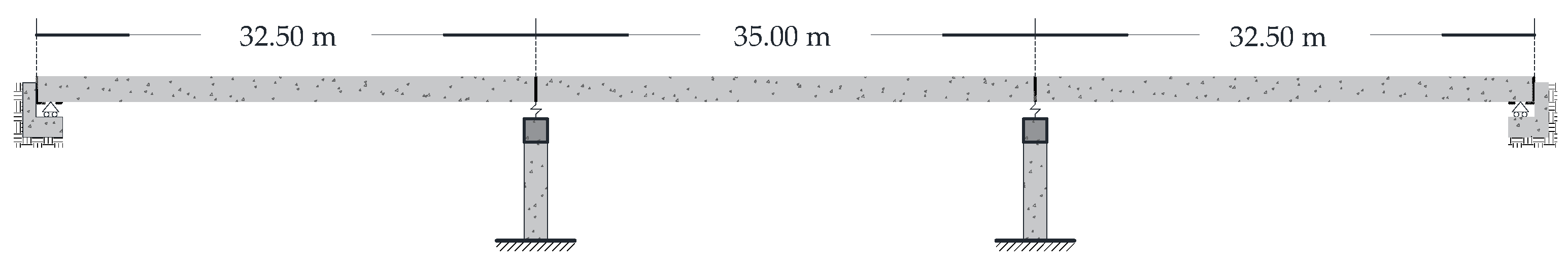
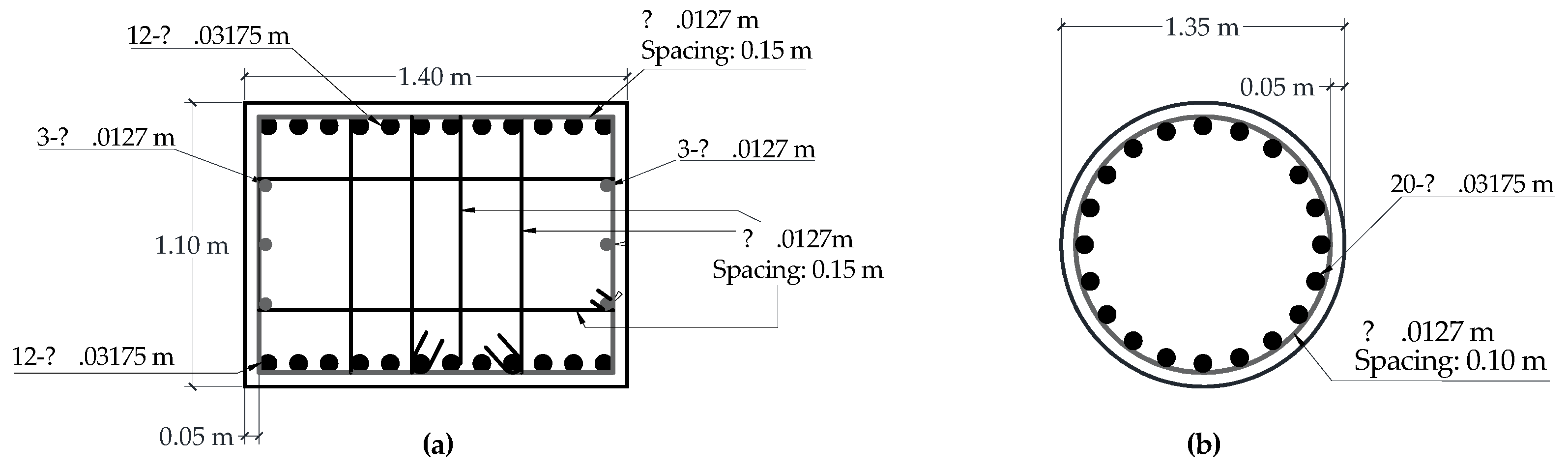
4. Example of Application

Reliability indicators are obtained for a continuous RC bridge of three spans with a total length of 100 m and 7 m in height. The compressive strength, f c , used for columns and cap beams is equal to 29.42 MPa, and has a value of 40 MPa for AASHTO beams. The structure, which is located in Acapulco, Guerrero, Mexico, is designed to accomplish a drift design equal to 0.004. The superstructure is supported by seat abutments located in the extreme spans. Fixed and roller supports are used at the base of columns and abutments, respectively. Beams and cap beams are connected by means of elastic springs with infinite stiffness in both longitudinal and transverse direction. The fundamental period of the RC bridge is equal to 0.40 s. Figure 1 and Figure 2 show the longitudinal and transverse sections of the bridge, respectively. Figure 3 shows the dimensions and reinforcement of the column and cap beams sections.

4.1. Expected Structural Properties of Materials, Loads, and Structural Sections

The expected properties refer to properties defined based on mean values from experiment tests. The use of expected structural properties is essential for providing an accurate measure of the expected response of the overall system. The intention is to avoid systematic bias by using nominal instead of expected properties for some structural components. Table 1 shows the statistical parameters for concrete strength, f c , recommended by [30].
The statistical parameters of the compressive strength, f c , of the concrete used in the bridge structure that are not included in Table 1 are obtained by means of linear interpolation. Regarding the yield stress of the reinforcing steel, the parameters proposed by [31] are used, which are shown in Table 2.
The ε s h value is the strain in the hardening zone and ε s u is the value of the ultimate strain of the reinforcing steel. The statistical parameters associated with dead load in reinforced concrete bridges are defined by [30]. The results of this research are shown in Table 3. Table 4 shows the mean values for structural sections of the bridge [32].

4.2. Nonlinear Dynamic Procedure
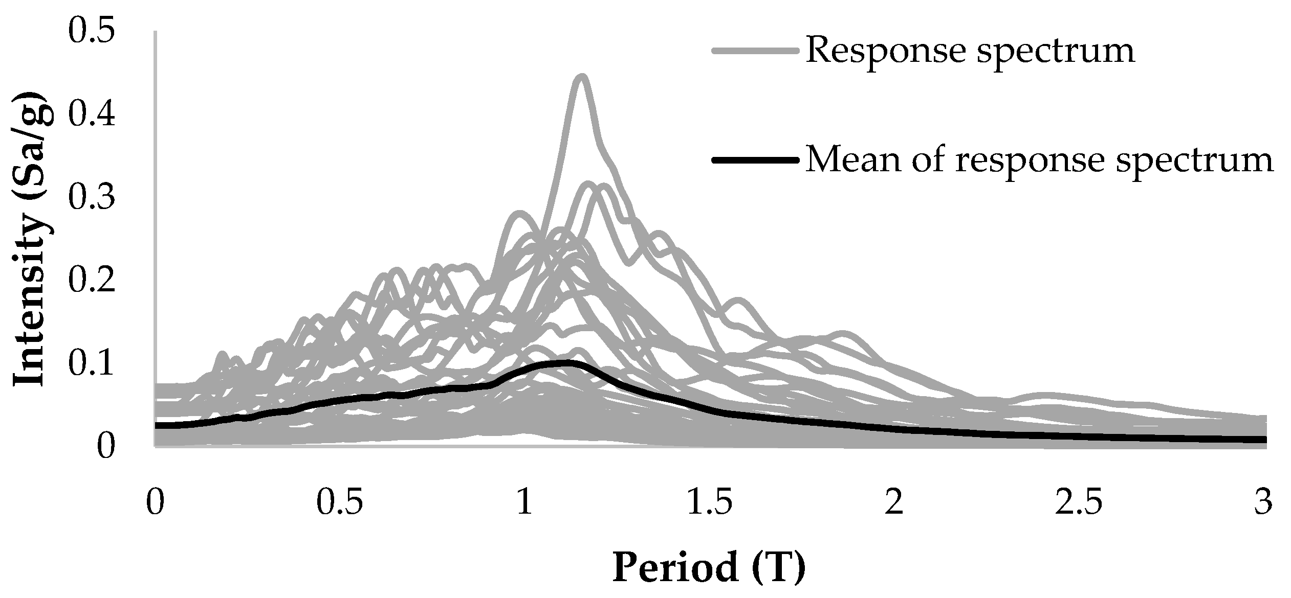
Nonlinear analysis is the best tool currently available for predicting structural response at varying levels of ground motion intensity. The nonlinear dynamic analysis aims to estimate all significant modes of deformation and damage in the structure, from the onset of inelastic response to the collapse. To compute structural performance from a probabilistic point of view, nonlinear response analysis is based on the expected properties of materials and components (see Section 4.1). In Mexico, most bridges are designed to undergo certain nonlinear behavior under extraordinary earthquake action. As for the bridge topology in the study, columns resist lateral loadings; they provide the lateral stiffness of the system. Collapse is considered to occur when plastic hinges appear at the ends of columns and cap beams. The bridge deck is considered to transmit dead loads only. The moment–curvature relation for each structural element is estimated considering the stress–strain constitutive model of confined reinforced concrete reported by [33] and [31] for Mexican steels. The cyclic model developed by [34], called the modified Takeda hysteresis rule, is used. The parameters α and β that consider the stiffness degradation of such hysteresis rule are equal to 0.5 and 0.6. The Ruaumoko 3D program [35] is used to compute the nonlinear response of the structural system.

4.3. Ground Motions

The National Seismological System of Mexico has an earthquake monitoring network in the state of Guerrero due to its location as seismic zone in the southwest of the Mexican Republic. For this study, two stations near the analyzed bridge are identified: a) “Acapulco Centro Cultural”, ACAC, and “Acapulco Diana”, ACAD, where the information was collected to integrate a database of 40 seismic records with magnitudes between 4 and 7.5. The dominant period of soil site presents values from 0.3 to 0.64, the maximum ground acceleration of the ground motions ranges from 0.019 to 0.44 Sa/g, and the mean of epicentral distance is 170 km. Figure 4 shows the pseudoacceleration spectrum of the 40 seismic records and their mean. Table 5 shows the characteristics of all the seismic records used in the analysis.

4.4. Structural Capacity Estimation

The nonlinear analysis is computed to estimate the structural behavior using incremental dynamic analysis (IDA); forty capacity curves associated with the seismic records of ACAD and ACAC are obtained. Figure 5 shows that the IDA curves have three phases: (1) structural elastic behavior, (2) inelastic response zone, and (3) the point near failure, which is identified with a black dot. Considering that the incipient failures follow a lognormal distribution [28,29], the median value of the structural capacity results in 0.0114 with a standard deviation of the natural logarithm of the capacity, σ l n C , of 0.18.

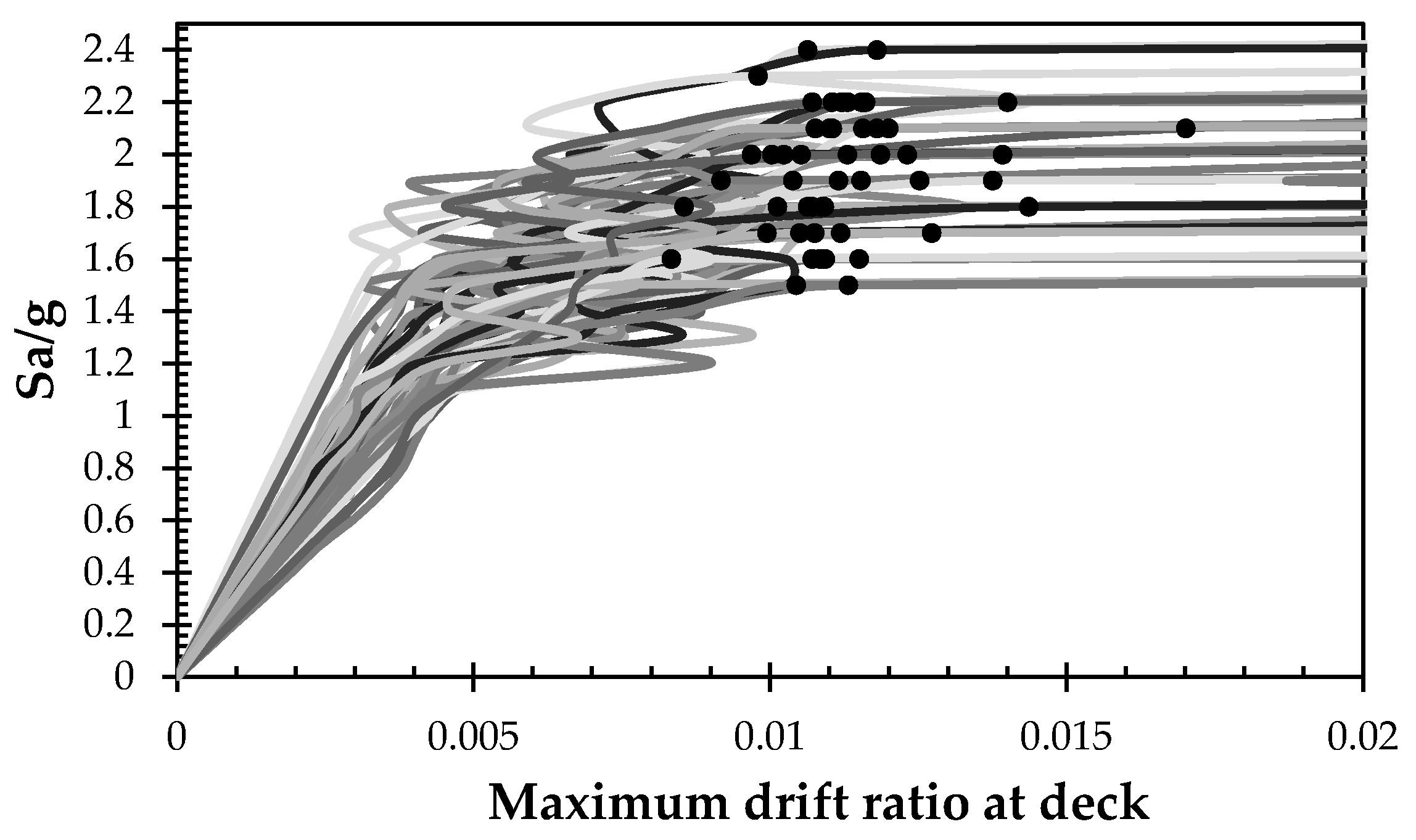
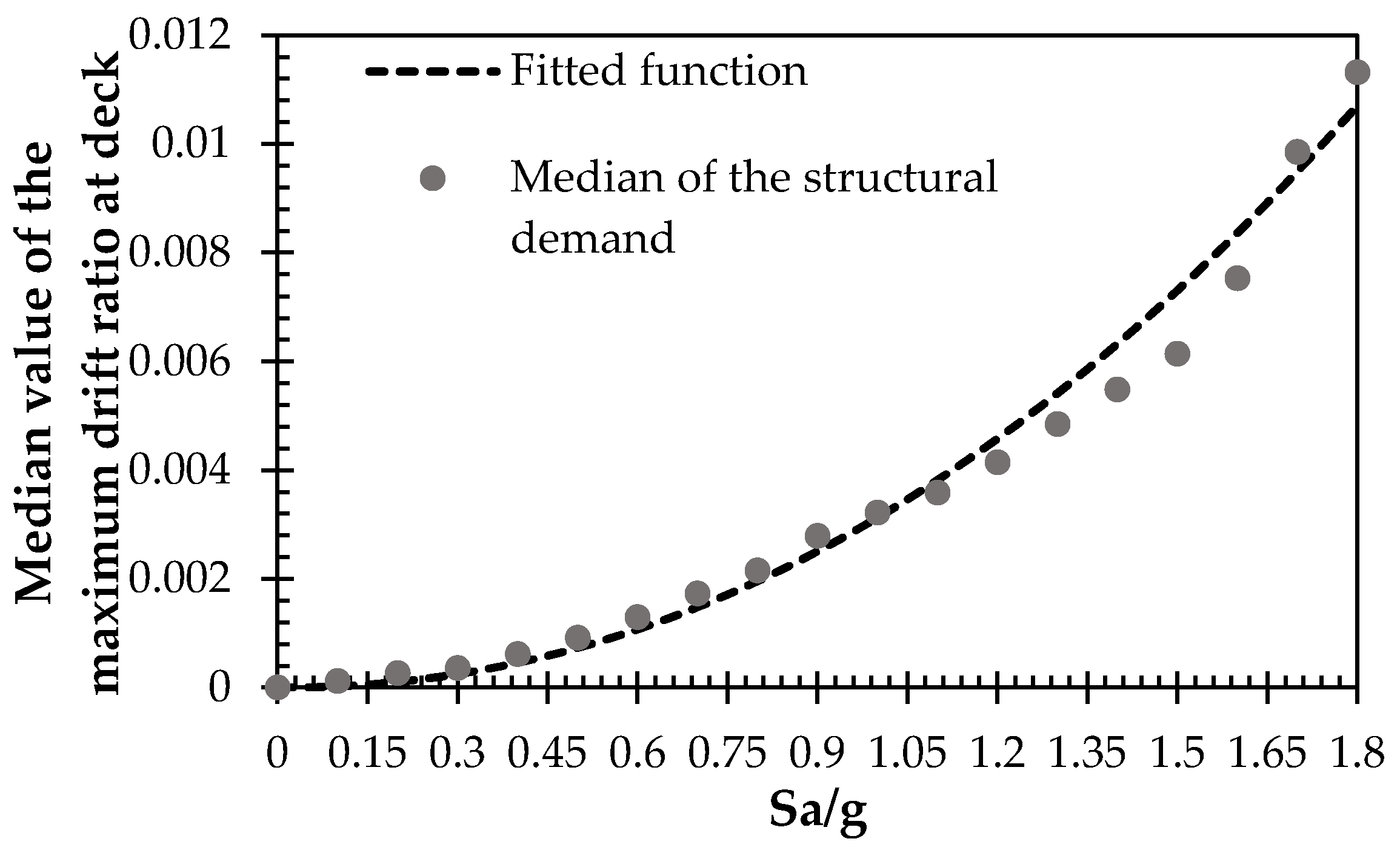
4.5. Structural Demand Assessment

The median structural demand, D ^ , is calculated by means of step-by-step nonlinear dynamic analyses, considering forty seismic records shown in Table 5. The seismic records are scaled up until failure of the structure occurs. Figure 6 shows the median of the structural demand and the fitted function. For this case, the parameters that fitted the shape of the structural demand are a = 0.00313 and b = 2.0921 . The following is observed: (a) the median of structural demand increases proportionally to the seismic intensities; (b) seismic intensities less than 0.45 Sa/g do not generate any structural damage.
Table 5. Characteristics of 40 seismic records.
“Acapulco Centro Cultural”, ACAC“Acapulco Diana”, ACAD
CNIDDateMagnitudeCNIDDateMagnitude
19509-141/N00E09/14/956.4211112-111/N00E12/11/116.5
29509-141/N90E09/14/956.4221112-111/N90E12/11/116.5
30205-281/N90E05/28/024.9239509-141/N00E09/14/956.4
40205-281/N00E05/28/024.9249509-141/N90E09/14/956.4
50206-191/N90E06/19/025.5259701-111/N00E01/11/976.9
60206-191/N00E06/19/025.5269701-111/N90E01/11/976.9
70209-251/N90E09/25/024.7279906-151/N00E06/15/996.4
80301-221/N90E01/22/035.6289906-151/N90E06/15/996.4
90401-011/N00E01/01/045.7299909-301/N00E09/30/997.5
100401-012/N90E01/01/045.8309909-301/N90E09/30/997.5
110401-012/N00E01/01/045.8310007-211/N90E07/21/005.1
120401-131/N00E01/13/045.1320401-011/N90E01/01/045.7
130406-141/N00E06/14/045.6330608-111/N90E08/11/065.9
140411-151/N00E11/15/044.7341105-051/N90E05/05/115.5
150508-141/N00E08/14/054.8351105-051/N00E05/05/115.5
160608-111/N00E08/11/065.9361112-111/N90E12/11/116
170905-221/N90E05/22/095.7371112-111/N00E12/11/116
181005-251/N00E05/25/105381306-271/N90E06/27/134
191006-301/N90E06/30/106391308-161/N90E08/16/135.1
201306-161/N90E06/16/135.8401308-161/N00E08/16/135.1

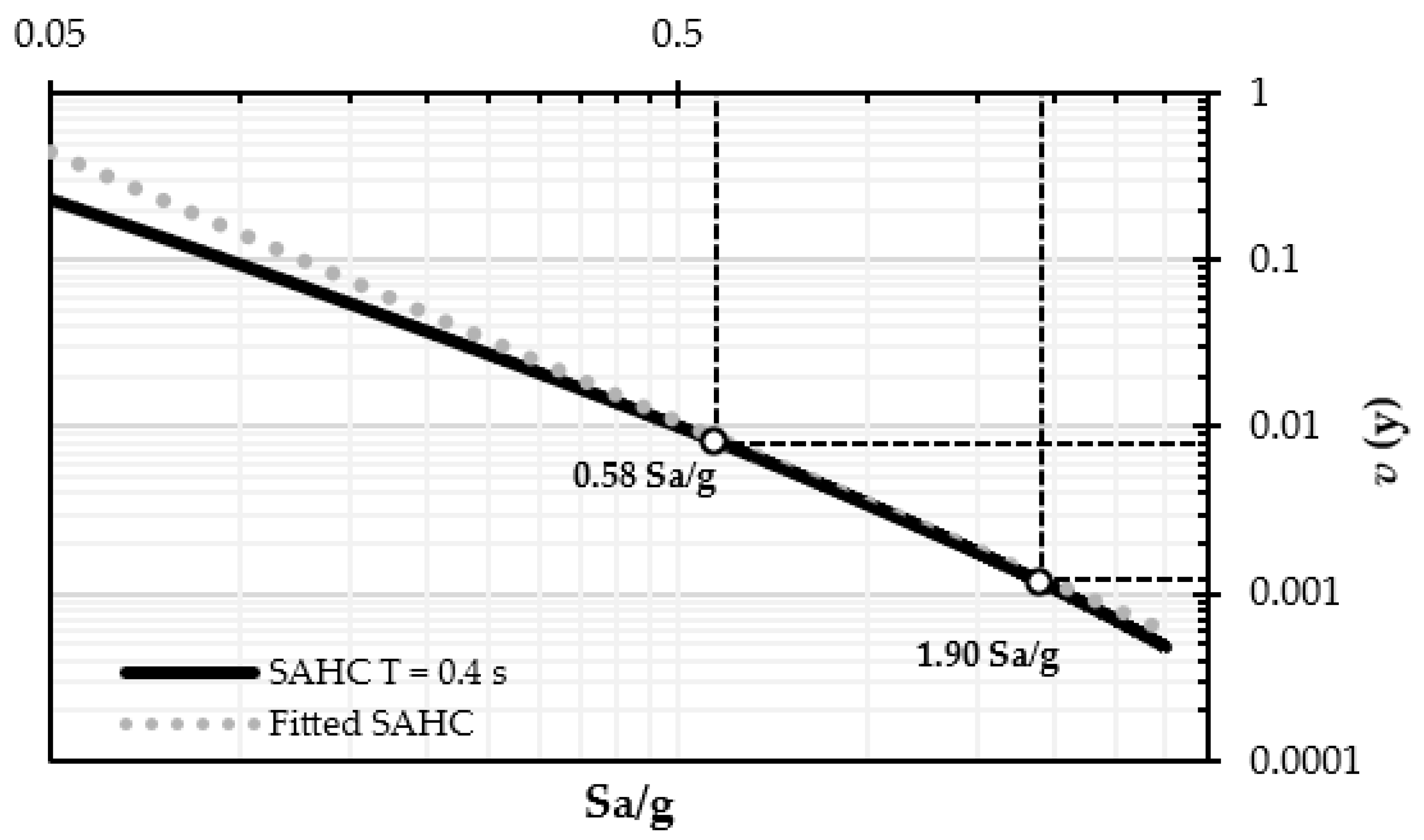
4.6. Spectral Acceleration Hazard

The spectral acceleration hazard curve (SAHC) is known, and it is associated with the fundamental period of the structure (T = 0.40 s), the site, and 5% of critical damping. The SAHC is fitted for the region of interest that corresponds to drift ratio values from 0.001 to 0.012, which are shown in Figure 7; their corresponding Sa/g are equal to 0.58 and 1.90. Such values represent the region of interest. Therefore, the constants k and r are equal to 0.003513 and 1.6224, respectively.

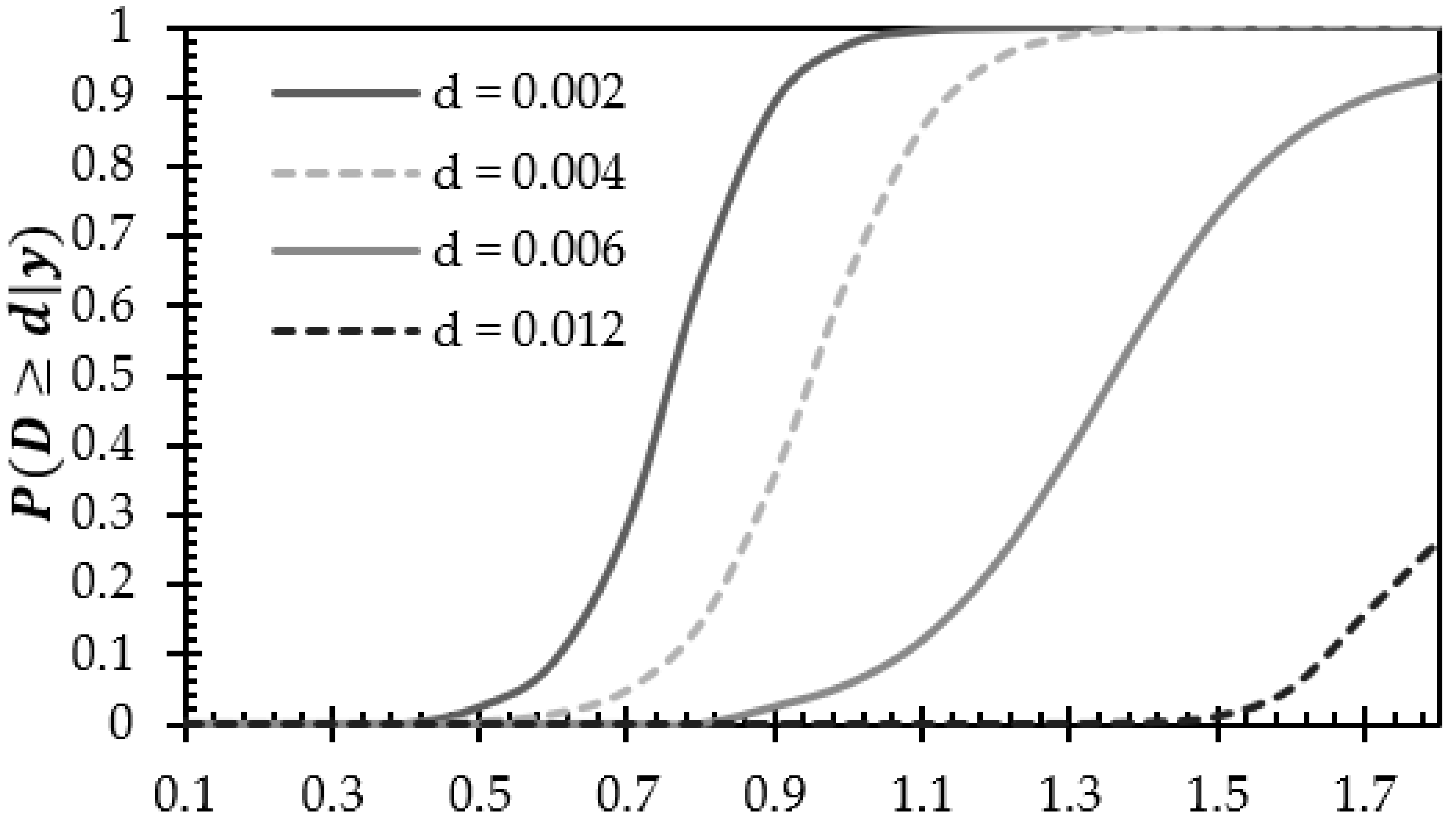
4.7. Probability of Exceeding a Certain Drift Threshold

Fragility curves are used to assess the vulnerability of structures due to a certain environmental load. It is assumed that fragility curves follow a lognormal shape with the following expression [36]:
P ( D d | y ) = 1 Φ ( l n d l n D ^ | y σ l n D ^ | y )  
where D ^ | y is the median value of the structural demand given a seismic intensity, y ; and σ l n D ^ | y is the standard deviation of the natural logarithm of the demand for a given intensity, y .
Fragility curves are calculated for four different drift thresholds: (a) 0.002, which is associated with a threshold lower than the design threshold, (b) 0.004, corresponding to the drift design and serviceability limit state [36], (c) 0.006, chosen as an intermediate threshold between serviceability and collapse thresholds, and (d) 0.012, which is associated with the value of collapse limit state [37]. Figure 8 shows the fragility curves for different drift thresholds. The following is observed: (a) seismic intensities less than 0.4 Sa/g produce exceedance probabilities close to zero in all thresholds; (b) regarding the threshold of 0.002, there are probabilities of exceedance of 1 when seismic intensities are greater than 1 Sa/g; (c) the serviceability threshold presents a value of exceedance probability of 0.5 at 0.95 Sa/g, approximately; (c) the serviceability threshold presents a value of exceedance probability of 0.5 at 0.95 Sa/g, approximately; (d) for the 0.006 threshold, and for intensities less than 0.8 Sa/g, there are exceedance probabilities close to zero; (e) for the threshold of 0.012, the exceedance condition is associated with a probability equal to 0.31 Sa/g.

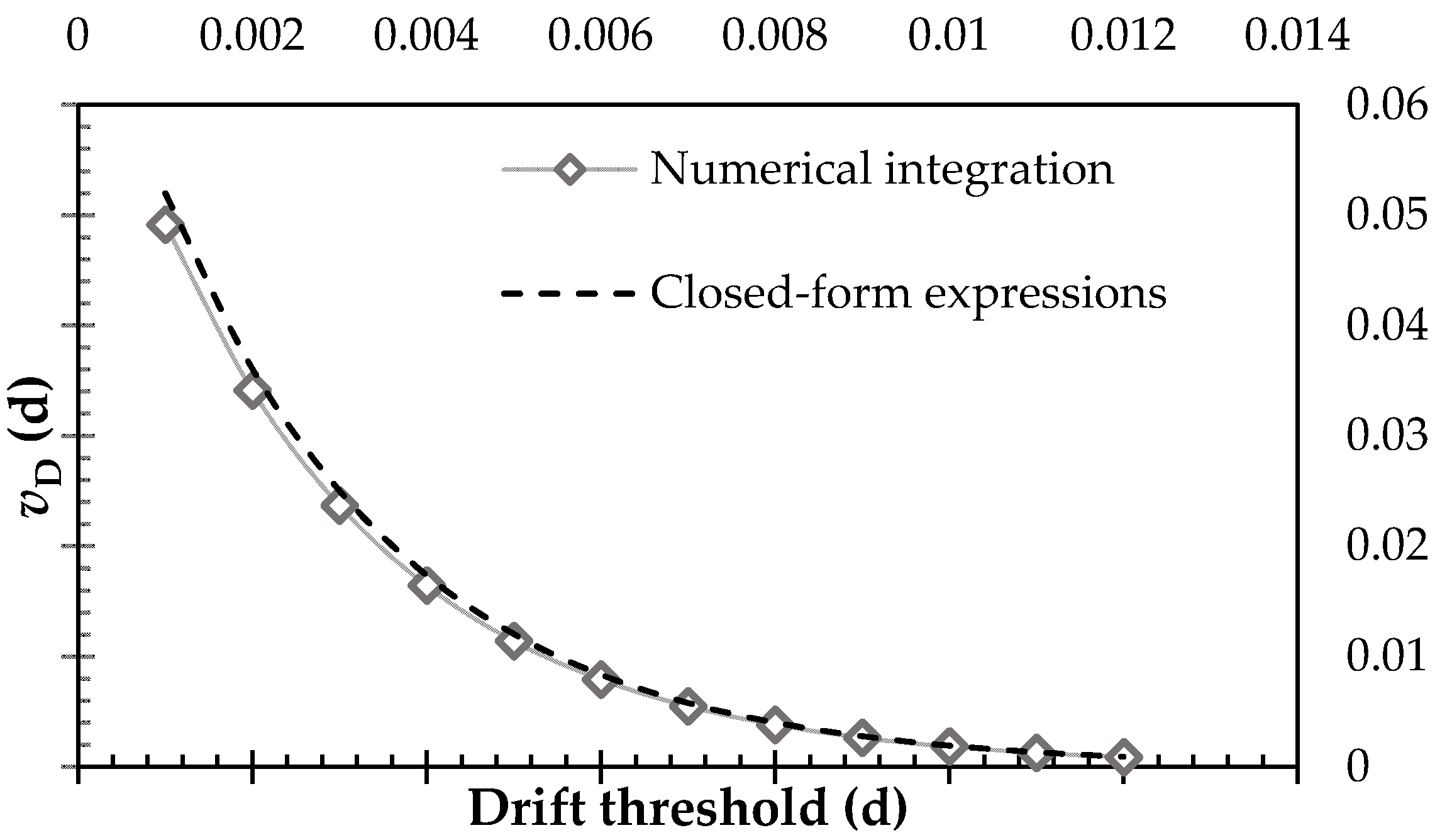
4.8. Mean Annual Demand Exceedance Rate

Demand hazard curves indicate the number of times that a certain drift threshold is exceeded per unit of time. The inverse of a certain value of demand hazard is the return period; this implies how many years a level of damage is expected to be exceeded. The above results are helpful for decision-making processes when the limit state under consideration is reached. Figure 9 illustrates the demand hazard curves obtained by closed-form expressions considering aleatory and epistemic uncertainties Equation (9) and numerical integration Equation (7). The mean annual rate of exceedance of the minimum intensity, v , is equal to 0.2308. The parameters a and b are obtained in Section 4.5, while parameters k and r are defined in Section 4.6. Epistemic uncertainties are considered with a value of 0.25 [38]. Demand hazard curves are built considering the maximum drift at the bridge deck for values from 0.001 to 0.012. In general, a difference of 5% between the two proposed approaches is observed. Such difference is mainly associated with the following: (a) epistemic uncertainties were considered in the closed-form expression, whereas the numerical solution does not consider such kind of uncertainties; and (b) there might be a bias when SAHC is fitted. If the values given by the closed-form expression are considered, a return period of 28 years is observed for threshold equal to 0.002, implying a mean annual demand rate of 0.03608; on the other hand, a mean annual demand frequency of 0.01738 is obtained for the serviceability limit state, which is associated with a return period of 58 years. For threshold d = 0.006 , a mean annual demand rate of 0.00837 is obtained, which is associated with a return period of 119 years, whereas a mean annual exceedance rate of 0.000935 is obtained for the limit state of collapse, implying a return period of 1068 years. Thus, it is inferred that it takes a long time to exceed higher drift thresholds.

4.9. Reliability Index

The reliability index β , Equation (6), the probability of failure, Equation (4), and the annual failure rate, Equation (2) are calculated with and without epistemic uncertainties; most of the parameters used are defined in the preceding section. The structural capacity, C ^ , is estimated in Section 4.4. Table 6 shows the reliability indicators computed considering the first service-life year with and without epistemic uncertainties. The following is observed: (a) the annual structural failure rate with epistemic uncertainties resulted 16.10% greater than the case without; (b) the return period of the mean annual rate of failure is 653 years after the bridge construction with epistemic uncertainties, and 759 years for the case without; (c) the reliability index decreases 1.66% when epistemic uncertainties are considered. Moreover, it is noticed that the reliability indices are lower than 3.5, which means that these values are not recommended by [39].

5. Conclusions

An approach was proposed to obtain both the reliability index and the probability of failure that considers epistemic uncertainties. Demand hazard curves are also obtained based on numeric and closed-form expressions. The probability of failure is proposed in a closed-form expression format, which has the following advantages: (a) it can be used for different kinds of structures; (b) it can be adapted for different environmental loads; (c) it calculates the probability of failure with and without the consideration of the epistemic uncertainties; and (d) it is familiar to structural engineers.
The approach was illustrated in a continuous bridge designed to comply with a drift threshold equal to 0.004. Uncertainties related to mechanical and geometric properties were considered, together with uncertainties for seismic loadings. Prior to obtaining demand hazard curves, different fragility curves were generated considering different thresholds. Demand hazard curves were determined for drift thresholds between 0.001–0.012. Considering the stipulations in the AASHTO design code [39], the lifespan of bridges must be guaranteed up to 75 years. Based on the results, the serviceability limit state could be exceeded 17 years before reaching the structure lifespan, which means that the design drift threshold is expected to be exceeded at 58 years. Therefore, the use of a design drift threshold equal to 0.004 is not recommended. A drift threshold exceedance does not mean that the structure is unable to resist seismic loadings; such exceedance means that the structure could present undesirable reliability levels before the recommended interval of serviceability. The reliability index target for bridges is to overcome β = 3.5, considering the structure as new [39]. Considering such target, the bridge under study presented a reliability index 18.24% lower than the recommendation given by [38] when epistemic uncertainties are considered; if such uncertainties are not considered, the reliability index is 16.28% lower. Thus, the value of 0.004 of design drift threshold is not recommended for this type of topology. It is recommended to explore lower values of design drift threshold between 0.001 to 0.003.
The reliability index and its probability of failure give certainty about both the safety level that a structure has under design loads, and the capacity of the structure to present serviceability levels during a certain time interval. The exceedance demand rate provides the instant when the structure reaches a certain level of damage. If the damage level compromises the structural integrity, decisions need to be made about inspection or maintenance actions with the aim to extend the lifespan of the system.

Author Contributions

Conceptualization, D.T.; methodology, D.T., D.H. and G.V.; software, D.H. and G.V.; validation, D.T., D.H. and G.V.; data curation, D.H. and G.V.; writing—original draft preparation, D.H. and G.V.; writing—review and editing, D.T., D.H. and G.V.; funding acquisition, D.T. All authors have read and agreed to the published version of the manuscript.

Funding

This research was funded by Consejo Nacional de Ciencia y Tecnología Grant A1-S-8700.

Institutional Review Board Statement

Not applicable.

Informed Consent Statement

Not applicable.

Data Availability Statement

Data is contained within the manuscript.

Acknowledgments

The first and second author gratefully acknowledge economic support from CONACyT during their PhD studies. They also appreciate the support of Universidad Autónoma Metropolitana (UAM). The third author appreciates the support given by both Consejo Nacional de Ciencia y Tecnología through the Ciencia Básica Project CB 2017-2018 A1-S-8700, and Universidad Autónoma Metropolitana.

Conflicts of Interest

The authors declare no conflict of interest.

References

  1. Echard, B.; Gayton, N.; Lemaire, M.; Relun, N. A combined Importance Sampling and Kriging reliability method for small failure probabilities with time-demanding numerical models. Reliab. Eng. Syst. Saf. 2013, 111, 232–240. [Google Scholar] [CrossRef]
  2. Huang, X.; Chen, J.; Zhu, H. Assessing small failure probabilities by AK-SS: An active learning method combining Kriging and Subset Simulation. Struct. Saf. 2016, 59, 86–95. [Google Scholar] [CrossRef]
  3. Decò, A.; Frangopol, D.M. Risk assessment of highway bridges under multiple hazards. J. Risk Res. 2011, 14, 1057–1089. [Google Scholar] [CrossRef]
  4. Lokuge, W.; Wilson, M.; Tran, H.; Setunge, S. Predicting the probability of failure of timber bridges using fault tree analysis. Struct. Infrastruct. Eng. 2019, 15, 783–797. [Google Scholar] [CrossRef]
  5. Hirzinger, B.; Adam, C.; Oberguggenberger, M.; Salcher, P. Approaches for predicting the probability of failure of bridges subjected to high-speed trains. Probabilistic Eng. Mech. 2020, 59, 103021. [Google Scholar] [CrossRef]
  6. Wang, R.; Leander, J.; Karoumi, R. Fatigue reliability assessment of steel bridges considering spatial correlation in system evaluation. Struct. Infrastruct. Eng. 2021, 6, 1–15. [Google Scholar] [CrossRef]
  7. Xia, H.W.; Ni, Y.Q.; Wong, K.Y.; Ko, J.M. Reliability-based condition assessment of in-service bridges using mixture distribution models. Comput. Struct. 2012, 106–107, 204–213. [Google Scholar] [CrossRef]
  8. Lü, Q.; Chan, C.L.; Low, B.K. System reliability assessment for a rock tunnel with multiple failure modes. Rock Mech. Rock Eng. 2013, 46, 821–833. [Google Scholar] [CrossRef]
  9. Frangopol, D.M.; Dong, Y.; Sabatino, S. Bridge life-cycle performance and cost: Analysis, prediction, optimisation and decision-making. Struct. Infrastruct. Eng. 2017, 13, 1239–1257. [Google Scholar] [CrossRef]
  10. Yuhua, D.; Datao, Y. Estimation of failure probability of oil and gas transmission pipelines by fuzzy fault tree analysis. J. Loss Prev. Process Ind. 2005, 18, 83–88. [Google Scholar] [CrossRef]
  11. Celarec, D.; Vamvatsikos, D.; Dolšek, M. Simplified estimation of seismic risk for reinforced concrete buildings with consideration of corrosion over time. Bull. Earthq. Eng. 2011, 9, 1137–1155. [Google Scholar] [CrossRef]
  12. Vamvatsikos, D.; Dolšek, M. Equivalent constant rates for performance-based seismic assessment of ageing structures. Struct. Saf. 2011, 33, 8–18. [Google Scholar] [CrossRef]
  13. Tolentino, D.; Ruiz, S.E.; Torres, M.A. Simplified closed-form expressions for the mean failure rate of structures considering structural deterioration. Struct. Infrastruct. Eng. 2012, 8, 483–496. [Google Scholar] [CrossRef]
  14. Tolentino, D.; Ruiz, S.E. Time-dependent confidence factor for structures with cumulative damage. Earthq. Spectra 2015, 31, 441–461. [Google Scholar] [CrossRef]
  15. Mackie, K.; Stojadinović, B. Probabilistic seismic demand model for California highway bridges. J. Bridg. Eng. 2001, 6, 468–481. [Google Scholar] [CrossRef] [Green Version]
  16. Dall’asta, A.; Tubaldi, E.; Ragni, L. Influence of the nonlinear behavior of viscous dampers on the seismic demand hazard of building frames. Earthq. Eng. Struct. Dyn. 2016, 45, 149–169. [Google Scholar] [CrossRef]
  17. Liu, X.X.; Wu, Z.Y.; Liang, F. Multidimensional performance limit state for probabilistic seismic demand analysis. Bull. Earthq. Eng. 2016, 14, 3389–3408. [Google Scholar] [CrossRef]
  18. Fanaie, N.; Sadegh Kolbadi, M.; Afsar Dizaj, E. Probabilistic Seismic Demand Assessment of Steel Moment Resisting Frames Isolated by LRB. Numer. Methods Civ. Eng. J. 2017, 2, 52–62. Available online: http://nmce.kntu.ac.ir/article-1-127-en.html (accessed on 1 September 2021). [CrossRef]
  19. Yee, E. Use of the t-Distribution to Construct Seismic Hazard Curves for Seismic Probabilistic Safety Assessments. Nucl. Eng. Technol. 2017, 49, 373–379. [Google Scholar] [CrossRef]
  20. Gavabar, S.G.; Alembagheri, M. Structural demand hazard analysis of jointed gravity dam in view of earthquake uncertainty. KSCE J. Civ. Eng. 2018, 22, 3972–3979. [Google Scholar] [CrossRef]
  21. Deylami, A.; Mahdavipour, M.A. Probabilistic seismic demand assessment of residual drift for Buckling-Restrained Braced Frames as a dual system. Struct. Saf. 2016, 58, 31–39. [Google Scholar] [CrossRef]
  22. Afsar Dizaj, E.; Fanaie, N.; Zarifpour, A. Probabilistic seismic demand assessment of steel frames braced with reduced yielding segment buckling restrained braces. Adv. Struct. Eng. 2018, 21, 1002–1020. [Google Scholar] [CrossRef]
  23. Maleki, M.; Ahmady Jazany, R.; Ghobadi, M.S. Probabilistic seismic assessment of SMFs with drilled flange connections subjected to near-field ground motions. Int. J. Steel Struct. 2019, 19, 224–240. [Google Scholar] [CrossRef]
  24. Zaker Esteghamati, M.; Farzampour, A. Probabilistic seismic performance and loss evaluation of a multi-story steel building equipped with butterfly-shaped fuses. J. Constr. Steel Res. 2020, 172, 106–187. [Google Scholar] [CrossRef]
  25. Yang, S.I.; Frangopol, D.M.; Neves, L.C. Service life prediction of structural systems using lifetime functions with emphasis on bridges. Reliab. Eng. Syst. Saf. 2004, 86, 39–51. [Google Scholar] [CrossRef]
  26. Yang, S.I.; Frangopol, D.M.; Kawakami, Y.; Neves, L.C. The use of lifetime functions in the optimization of interventions on existing bridges considering maintenance and failure costs. Reliab. Eng. Syst. Saf. 2006, 91, 698–705. [Google Scholar] [CrossRef]
  27. Tobias, P.; Trindade, D. Applied Reliability, 3rd ed.; Chapman and Hall/CRC: New York, NY, USA, 2011. [Google Scholar]
  28. Cornell, C.A.; Jalayer, F.; Hamburger, R.O.; Foutch, D.A. Probabilistic Basis for 2000 SAC Federal Emergency Management Agency Steel Moment Frame Guidelines. J. Struct. Eng. 2002, 128, 526–533. [Google Scholar] [CrossRef] [Green Version]
  29. Rosenblueth, E.; Esteva, L. Reliability Basis for Some Mexican Codes. Spec. Publ. 1972, 31, 1–42. [Google Scholar]
  30. Nowak, A.S.; Rakoczy, A.M.; Szeliga, E.K. Revised Statistical Resistance Models for R/C Structural Components; American Concrete Institute: Farmington Hills, MI, USA, 2011. [Google Scholar]
  31. Rodríguez, M.; Botero, J. Comportamiento sísmico de estructuras considerando propiedades mecánicas de aceros de refuerzo mexicanos. Rev. Ing. Sísmica 1995, 1, 39–50. Available online: https://www.smis.mx/index.php/RIS/article/view/268 (accessed on 2 August 2021). [CrossRef]
  32. Ellinwood, B.; Galambos, T.V.; McGregor, J.G.; Cornell, C.A. Development of a Probability Based Load Criterion for American National Standard A58 Building Code Requirements for Minimum Design Loads in Buildings and Other Structures; NBS SPECIAL PUBLICATION 577; U.S. Department of Commerce: Washington, DC, USA, 1980.
  33. Mander, J.B.; Priestley, M.J.N.; Park, R. Theoretical stress-strain model for confined concrete. J. Struct. Eng. 1988, 114, 1804–1826. [Google Scholar] [CrossRef] [Green Version]
  34. Otani, S. Inelastic Analysis of R/C Frame Structures. J. Struct. Div. 1974, 100, 1433–1449. [Google Scholar] [CrossRef]
  35. Carr, A.J. RUAUMOKO 3D Volume 3: User Manual for the 3-Dimensional Version; University of Canterbury: Christchurch, New Zealand, 2003; Volume 3, p. 152. [Google Scholar]
  36. Tolentino, D.; Márquez-Domínguez, S.; Gaxiola-Camacho, J.R. Fragility assessment of bridges considering cumulative damage caused by seismic loading. KSCE J. Civ. Eng. 2020, 24, 551–560. [Google Scholar] [CrossRef]
  37. NTC. Normas Técnicas Complementarias del Reglamento de Construcciones del Distrito Federal. Gaceta Oficial, Mexico City (in Spanish), 6th ed.; Trillas: Ciudad de Mexico, Mexico, 2004. [Google Scholar]
  38. Bradley, B.A.; Dhakal, R.P.; Cubrinovski, M.; Mander, J.B.; MacRae, G.A. Improved seismic hazard model with application to probabilistic seismic demand analysis. Earthq. Eng. Struct. Dyn. 2007, 36, 2211–2225. [Google Scholar] [CrossRef] [Green Version]
  39. AASHTO. Standard Specifications for Highway Bridges; American Association of State Highway and Transportation Officials: Washington, DC, USA, 2012. [Google Scholar]
Figure 1. Longitudinal view.
Applsci 12 00206 g001
Figure 2. Cross-section view.
Applsci 12 00206 g002
Figure 3. Geometry and design: (a) cap beams and (b) columns.
Applsci 12 00206 g003
Figure 4. Response spectra and mean for 40 seismic records.
Applsci 12 00206 g004
Figure 5. Structural capacity due to earthquakes.
Applsci 12 00206 g005
Figure 6. Median of the maximum drift.
Applsci 12 00206 g006
Figure 7. Spectral acceleration hazard curve for the fundamental period, T = 0.40 s.
Applsci 12 00206 g007
Figure 8. Fragility curves for different drift thresholds.
Applsci 12 00206 g008
Figure 9. Demand hazard curves.
Applsci 12 00206 g009
Table 1. Compressive stress, f c , of ordinary concrete.
f c   ( MPa ) Bias FactorCoefficient of Variation
27.601.240.15
31.001.210.14
41.401.150.125
Table 2. Yield and ultimate stress of reinforcing steel.
f y ( MPa ) ε s h   ( mm / mm ) f u   ( MPa ) ε s u   ( mm / mm )
Mean440.02 0.0066 713.92 0.11
Standard deviation16.570.002216.280.012
Table 3. Bias factor and variation coefficient for structural and nonstructural elements.
Bias FactorCoefficient of Variation
Factory items1.030.08
Site elements1.050.10
Asphalt1.000.25
Non–structural elements1.03–1.050.08–0.01
Table 4. Statistical parameters for structural elements.
Mean (m)Standard Deviation (m)
Slab width 7.62 × 10−46.60 × 10−3
Beam height −5.33 × 10−36.35 × 10−3
Beam width 2.54 × 10−33.81 × 10−3
Columns dimensions1.52 × 10−36.35 × 10⁻³
Cover 8.13 × 10−34.32 × 10−3
Table 6. Reliability indicators.
E ( v F ) P F β
With epistemic uncertainties1.531 × 10−31.529 × 10−32.96
Without epistemic uncertainties 1.318 × 10−31.317 × 10−33.01
Publisher’s Note: MDPI stays neutral with regard to jurisdictional claims in published maps and institutional affiliations.

