Abstract
The traditional method for seismic earth pressure calculation has certain limitations for retaining structures under complex conditions. For example, when the soil width is small, the results obtained by the traditional method will be much larger. Therefore, this paper assumes that the soil slip surface is a logarithmic spiral. Based on the plane strain unified strength theory formula, while also considering the soil arching effects and tension cracks, the analytical solutions of the lateral earth pressure coefficient and the active earth pressure under the earthquake action were deduced. The mechanism and distribution of seismic active earth pressure with limited width were discussed in terms of some relevant parameters. The results indicated that the seismic active earth pressure presented a “convex” nonlinear distribution along the retaining structure. As the contribution of the intermediate principal stress increased, the strength limit of the material was effectively utilized, and the earth pressure was reduced by 22.96%. The resultant force increased as the horizontal seismic coefficient increased. However, this effect was no longer evident when the wall–soil friction angle was close to the internal friction angle. The resultant force action point increased with the wall–soil friction angle, and it should be noted that was true when . Finally, by drawing a comparison with previous studies, we verified that the method proposed in this paper is reasonable and can provide a new idea for subsequent 3D seismic earth pressure research.
1. Introduction
With the development of construction technology and the increase of underground building density, the soil behind deep foundation pit retaining structures will be restricted by many other types of underground structures. For example, in an existing deep basement, underground pipe gallery, or subway station, the soil is contained within a limited width. Earthquake is also a factor that must be considered. Retaining structures in high-intensity seismic areas are constantly facing the severe test of earthquake damage. Therefore, for the safety and economy of the retaining structure, the accurate estimation of the seismic earth pressure of the limited backfill is very important. Traditional Rankine [1], Coulomb [2], and Mononobe–Okabe [3,4] theories are based on semi-infinite space. The slip surface is assumed as a plane, and the effects of the intermediate principal stress and soil arching effects are not considered. Some scholars have also realized this problem, and many theoretical and experimental studies have been carried out.
At present, the earth pressure distributions obtained by some theories commonly used in engineering are linear. However, related experimental and theoretical studies [5,6] have shown that the distribution is actually nonlinear. For soil with limited width, the magnitude and distribution of earth pressure given by some experiments and numerical studies [7,8,9] are also quite different from the traditional earth pressure theory. Tang and Chen [10] established a general calculation model and obtained an analytical solution for limited backfill. Xie et al. [11] studied the active earth pressure of the retaining wall near the rock face and proposed an analytical solution which can more accurately predict the earth pressure of the retaining wall near the rock face. Moreover, the influence of soil arching cannot be ignored. Since the earliest discovery of the arching effect by Terzaghi [12], many scholars have introduced soil arching effects into the calculation of earth pressure. Handy [13] proposed the lateral earth pressure coefficient and a formula for the nonlinear active earth pressure. Take and Valsangkar [14] conducted a series of centrifugal tests on the earth pressure of a retaining wall with a limited backfill width. Paik and Salgado [15] derived a method for the calculation of the lateral pressure coefficient based on soil arching effects. Zhao and Zhu [16] introduced the soil arching effects into limited backfill, and the results obtained were closer to the numerical analysis, which has a certain engineering reference value.
As mentioned earlier, traditional earth pressure theories are based on the assumption of a planar fracture surface. However, some studies [17,18] have shown that the slip surface of limited backfill is actually closer to a curve. Yang et al. [19,20] and He et al. [21] conducted experimental and theoretical studies of the limited backfill slip surface. The results showed that the slip surface is a logarithmic spiral, and the theoretical results were in good agreement with the experimental results. Seismic action must be paid sufficient attention. Based on Rankine’s theory, Iskander et al. [22] analyzed the seismic active earth pressure of cohesive soil in semi-infinite space using a pseudo-static method. The rationality of the method was verified by comparison with previous studies. Yang and Zhang [23] used the model of the combination of logarithmic spiral and tension cracks. The energy method was used to analyze the seismic active earth pressure under different crack types. In some statistics about the damage of supporting structures, the influence of earthquake action is very significant [24,25]. However, there are few studies on the seismic earth pressure of limited backfill.
Although the above works carried out studies on different aspects of earth pressure, they are all based on the traditional Mohr–Coulomb theory—that is, the effect of intermediate principal stress is ignored. The soil behind the wall is actually in a three-dimensional (3D) stress state. Li et al. [26,27] studied the active earth pressure coefficient in the 3D state and pointed out that consideration of the 3D effect of the soil will produce a more economical solution. Since the unified strength theory [28,29,30] was proposed, the important influence of intermediate principal stress on material failure has been considered. Zhang et al. [31] proposed an improved Rankine earth pressure formula based on the unified strength theory. The results were lower than those obtained using the classic Rankine theory, indicating that the unified strength theory can further exert the strength potential of materials. Jiao et al. [32] introduced the intermediate principal stress into the calculation of the semi-infinite earth pressure. The soil arching effects were considered. The results showed that the proposed method could effectively reduce material consumption and save engineering costs. Shao et al. [33] considered the relationship between the residual strength effect and the strength parameters of unsaturated loess, established the seismic passive earth pressure formula of the loess filling based on the modified plane strain unified strength theory.
In summary, the current research on seismic earth pressure mainly has the following deficiencies: (1) The influence of intermediate principal stress is ignored; (2) research on limited backfill needs to be supplemented; (3) most of is the existing research is still based on the assumption of a planar slip surface; and (4) there is little research on cohesive soil. Therefore, on the basis of previous studies, this paper assumes that the slip surface is a curve, considering the influence of intermediate principal stress, soil arching effects, and tension cracks. The active lateral pressure coefficient and the earth pressure formula of limited backfill under earthquake action are deduced, and the sensitivity of the main parameters is analyzed through calculation examples.
2. Unified Strength Theory Formula under Plane Strain State
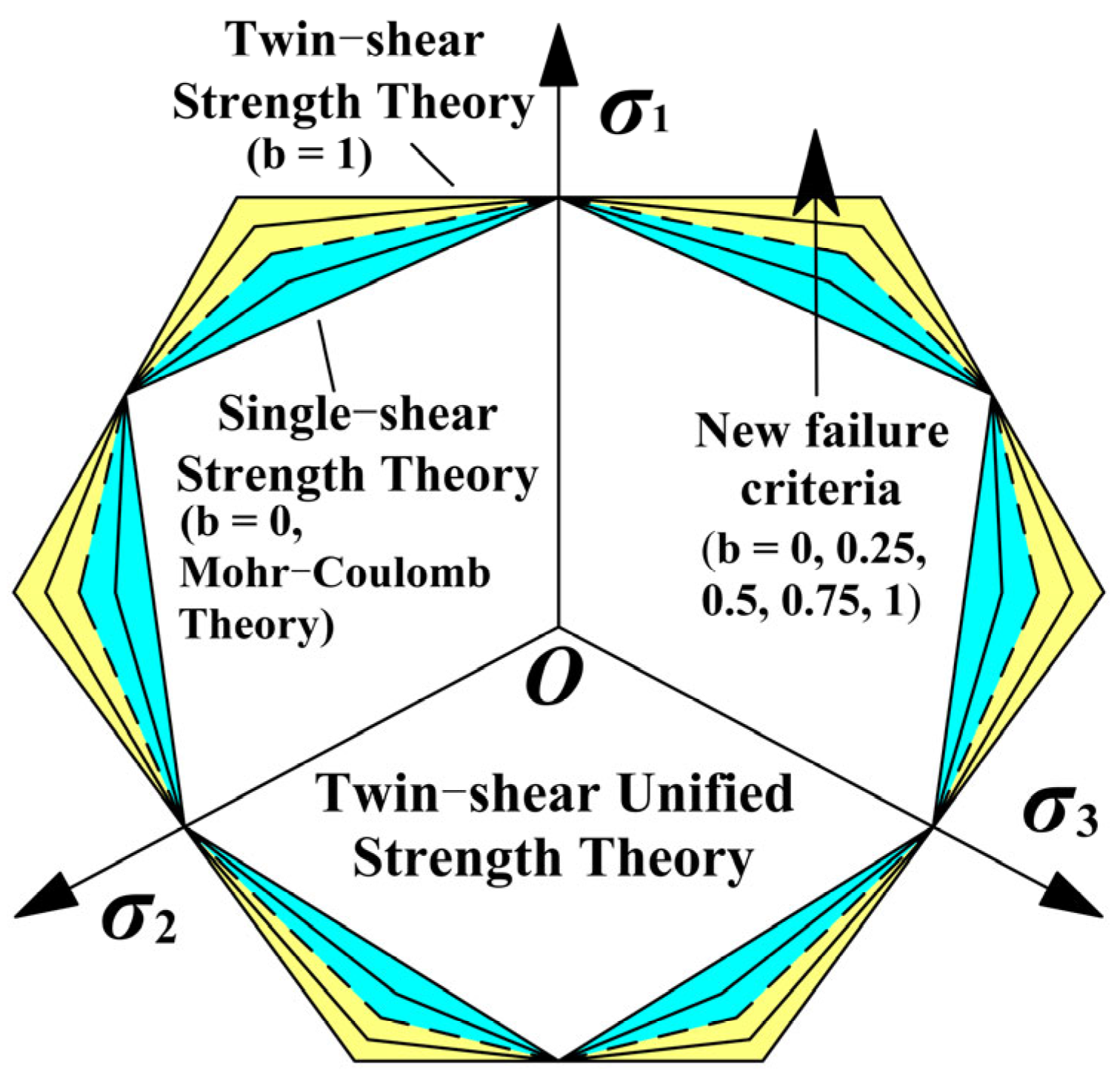
The intermediate principal stress has an important influence on the failure of different materials. The twin-shear unified strength theory was proposed, containing all the stress components acting on the orthogonal octahedron element and different effects on material failure [30]. In addition, it can adapt to geotechnical materials with different tensile and compressive strengths and related to hydrostatic stress, and makes up for the deficiencies of the Mohr–Coulomb theory. This theory collects a series of failure criteria, covering all areas between the upper and lower limits, and has good applicability to different materials. The principal stress form of the twin-shear unified strength theory is expressed as:
where is the intermediate principal stress weight coefficient, which can express the influence of the intermediate principal stress on the yield of the material, and [29]; , , are three principal stresses; and are the material tensile and compressive stress, respectively; is the material tension–compression ratio parameter; and and are the soil cohesion and internal friction angle obtained from the triaxial test, respectively.
The π plane limit lines of the unified strength theory are shown in Figure 1. The unified strength theory can degenerate to more calculation criteria under different values. The limit lines are convex when . When or , the limit lines are non-convex. Therefore, the unified strength theory is not limited by the traditional convexity theory. In addition to forming a series of convex limit surfaces, it can also form a series of non-convex limit surfaces, which can be flexibly adapted to various materials. The innermost is the single-shear strength theory—that is, the Mohr–Coulomb strength theory (). The outermost is the twin-shear strength theory ().
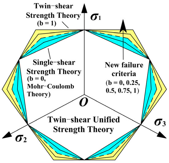
Figure 1.
Yield loci of the unified strength theory.
Because the intermediate principal stress is between the maximum principal stress and the minimum principal stress , the following relationship is given:
where is the intermediate principal stress coefficient. The elastic solution of the plane strain problem can be known: . Therefore, can be obtained by the generalized Hooke’s law: . In plane strain, volume deformation in the plastic state is ignored, that is, . Moreover, when , , the twin-shear unified strength theory is a special case or linear approximation of Tresca, Mises, and twin-shear stress yield criteria. Different values can reflect different intermediate principal stress effects. Therefore, is taken as the representative value in subsequent analysis, combined with the influence of the intermediate principal stress. By combining Equations (1) and (2), the modified soil friction angle and cohesion are determined as:
3. Slip Surface Equation of Limited Backfill
This paper is based on the theoretical and experimental research of Wang et al. [34] and Yang and Tang [19]. The cohesive backfill has a limited width. The slip surface of the backfill is assumed to be a logarithmic spiral, as shown in Figure 2.
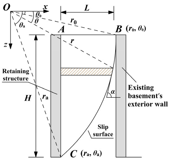
Figure 2.
Sketch of logarithmic spiral slip surface.
In Figure 2, is the retained soil width; is the retaining structure height; is the angle between the tangent line at any point on the slip surface and the horizontal plane; and and are the logarithmic spiral angle and polar radius at any point on the slip surface, respectively. and are the polar coordinates of the pending point.
The slip surface equation is given by:
The corresponding rectangular coordinate equation can be expressed as:
The slope of any point on the logarithmic spiral is:
Then, the angle between the tangent line at any point on the slip surface and the horizontal plane is:
at point C can be determined as:
where is the Coulomb failure angle when the soil reaches the active limit state, and . At this time, the active earth pressure required is biased towards safety [20].
4. Active Earth Pressure Analysis under Seismic Action
Earth pressure analysis under seismic action is a dynamic problem. In this paper, the pseudo-static method is used to deal with the calculation of dynamic earth pressure—that is, the Mononobe–Okabe theory. The seismic inertial force is applied to the sliding soil and then combined with the sliding soil to form an equivalent weight. It is made into a static problem. In order to simplify the calculation, the following assumptions are made:
- The soil surface is level.
- The supporting structure is rigid, and its deformation is not considered.
- The influence of the foundation pressure in the basement of the adjacent building is not considered [35].
- The horizontal seismic inertial force points to the retaining structure, and the vertical seismic inertial force points upwards.
- The effect of the earthquake on the basic mechanical properties of soil is not considered.
4.1. Seismic Active Lateral Pressure Coefficient for Cohesive Soil
Soil arching effects exist objectively [36,37], especially in limited soil and deep foundation pits. In the system under consideration in the present study, due to the lateral movement of the retaining structure and the influence of the wall–soil friction angle, the stress redistribution phenomenon will be more obvious (Figure 3a). In addition, this research is aimed at cohesive soil. Based on the research of Paik and Salgado [15], and combined with the Mohr circle for initial liquefaction given by Richards et al. [38], the stress Mohr circle when the soil behind the retaining structure reaches the active limit state under the earthquake is shown in Figure 3b.

Figure 3.
Arching effects in limited backfill: (a) trajectory of minor principal stress; (b) Mohr circle for stresses at the retaining structure.
In Figure 3, and are the angles between the minor principal stress surface and the horizontal plane at the retaining structure and the slip surface, respectively; is the radius of the minor principal stress arch; is the distance from any point inside the soil to the surface; is the thickness of the thin-layer element; is the uniform surcharge on the soil surface; is the vertical force at any point of the minor principal stress trajectory at depth ; is the shear stress on the retaining structure; is the wall–soil friction angle; is the vertical seismic coefficient; is the lateral earth pressure coefficient; and the other parameters are as mentioned above.
From Figure 3b, the following relationship is given:
where and are the stress values in the new and old coordinate systems, respectively.
When the soil reaches the active limit equilibrium state, combined with the stress Mohr circle, the principal stress deflection angle in the soil at the retaining structure can be obtained [15]:
where is the Rankine active earth pressure coefficient, and .
The angle between the action surface of the major principal stress and the failure surface is . Therefore, the angle between the minor principal stress surface and the horizontal plane at the slip surface can be given by:
As shown in Figure 3a, the average vertical stress acting on the thin-layer element can be obtained:
Additionally, from Figure 3b, and considering the uniform surcharge on the soil surface, the following is obtained:
where is the unit weight of the retained soil. Combining Equations (14) and (15), the seismic active lateral pressure coefficient for cohesive soil can be obtained:
In order to facilitate subsequent calculations, the following relationship is given:
where is the non-cohesive soil lateral earth pressure coefficient, which can be expressed as:
The influence of tension cracks in cohesive soil is a problem that must be considered. The height of tension cracks under earthquake ():
according to Equation (19), when , .
4.2. Establishment of Seismic Active Earth Pressure Formula
The thin-layer element method is used in this part. The selected element is shown in Figure 4. When the element thickness is sufficiently small, can be approximated as a straight line.
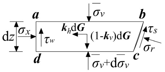
Figure 4.
Horizontal thin-layer element model.
In Figure 4, and are the average vertical stress acting on the top and bottom of the thin-layer element, respectively; and are the horizontal and vertical seismic coefficients, respectively; is the self-weight of the thin-layer element; is the horizontal reaction force of the retaining structure; is the reaction force of the lower soil body to the upper soil; and is the shear stress at the slip surface.
The self-weight of the element is (higher-order infinitesimals omitted):
The shear stresses on both sides of the element are taken as:
where is the adhesion between the retaining structure and soil.
The stress equilibrium equation in the horizontal and vertical directions of the thin-layer element are:
By combining Equations (20)–(23) and with higher-order infinitesimals omitted, the following differential equation is obtained:
where
Equation (24) is solved with the following boundary condition,, yielding:
where
In summary, the distribution formula of the seismic active earth pressure can be expressed as:
4.3. Resultant Force and Its Action Point
By combining Equations (16) and (26), the horizontal active earth pressure resultant force can be obtained as:
where ; can be determined as . Using the optimization algorithm to find the number that makes achieve the maximum value is the required , and the horizontal active earth pressure resultant force can also be obtained accordingly.
The total overturning moment of the retaining structure can be expressed as:
The resultant force and its action point are respectively determined as:
Using the formula in this paper to calculate the active earth pressure of limited backfill, the main calculation process diagram is shown in Figure 5.
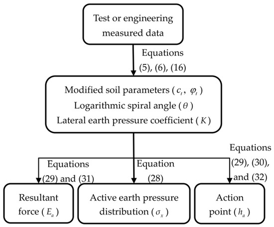
Figure 5.
Flow chart of active earth pressure calculation.
5. Parametric Sensitivity Analysis
Relevant important parameters are discussed according to the listed calculation route. In the following analysis, the basic parameters of the soil were uniformly selected as unit weight , cohesion , internal friction angle , retaining structure height , soil width , uniform surcharge . We mainly discuss the influence of intermediate principal stress weight coefficient , horizontal and vertical seismic coefficients and , wall–soil friction angle , and soil width on the earth pressure distribution, lateral earth pressure coefficient, active earth pressure resultant force, and its action point.
5.1. Active Earth Pressure Distribution
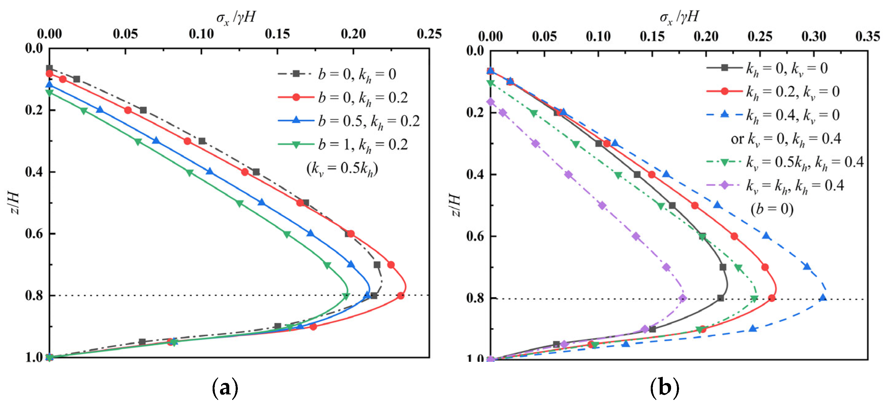
We assumed that the wall–soil , and that the intermediate principal stress weight coefficient . According to the Specification of Seismic Design for Highway Engineering (JTG B02-2013) [39], the following parameter values were set: horizontal seismic coefficient = 0, 0.2 (level VIII), 0.4 (level IX); vertical seismic coefficient . The horizontal seismic active earth pressure distributed along the height of the retaining structure is shown in Figure 6. Horizontal active earth pressure and depth are dimensionless.
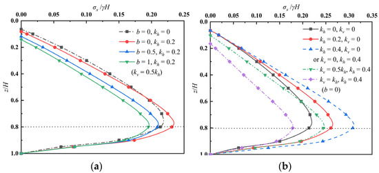
Figure 6.
Distribution of horizontal seismic active earth pressure: (a) ; (b) and .
Figure 6a shows the horizontal active earth pressure distribution under different intermediate principal stress weight coefficients. Where , it can be seen that as the values increased, the horizontal active earth pressure gradually decreased. It is worth noting that in the working condition without earthquake action (i.e., ), the intermediate principal stress was not considered. The obvious difference indicates that the seismic action significantly influenced the earth pressure compared with other working conditions. In addition, it can be seen from Figure 6b that when , the horizontal active earth pressure gradually increased with the horizontal seismic coefficient, and the trend of non-linearity increased sharply. The main gaps were concentrated in the middle and lower parts of the retaining structure. On the contrary, as the vertical seismic coefficient increased, the horizontal active earth pressure demonstrated a clear and gradual decreasing trend. Under several working conditions, the distribution of active earth pressure presented the same trend, and the decreasing points were all near .
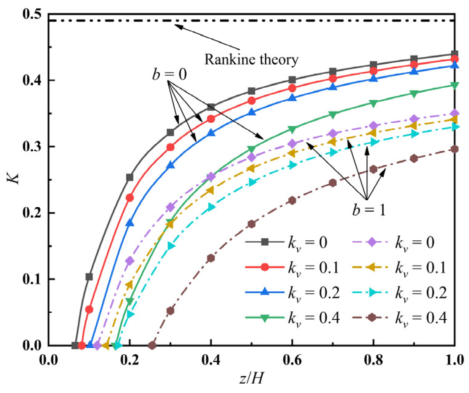
5.2. Lateral Seismic Active Earth Pressure Coefficient
The lateral seismic active earth pressure coefficient is the key to calculating the earth pressure, which is affected by many factors. That is:
In this study, ; . The change curves of under different depths and vertical seismic coefficient are shown in Figure 7. It can be seen that under several working conditions, along the depth direction, showed a sharp increasing trend in the middle and upper parts of the retaining structure, and then the increase rate tended to become flat. Affected by the tension cracks, had a negative value within a certain range of the soil surface, and the overall coefficient was smaller than the Rankine earth pressure coefficient. In addition, gradually decreased with the increase of and . When , the reduction was the most obvious.
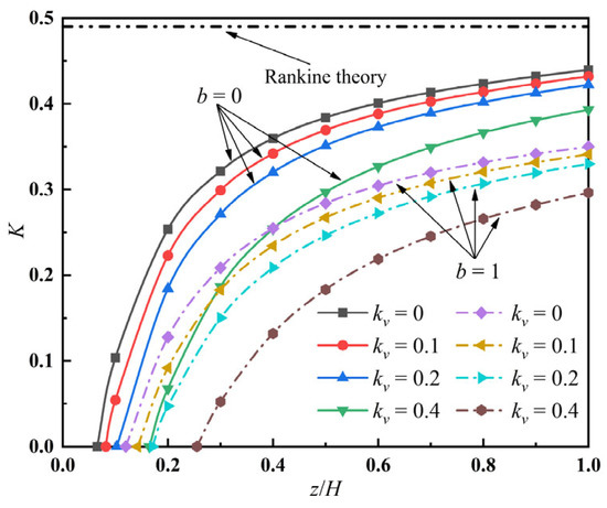
Figure 7.
Influence of and on .
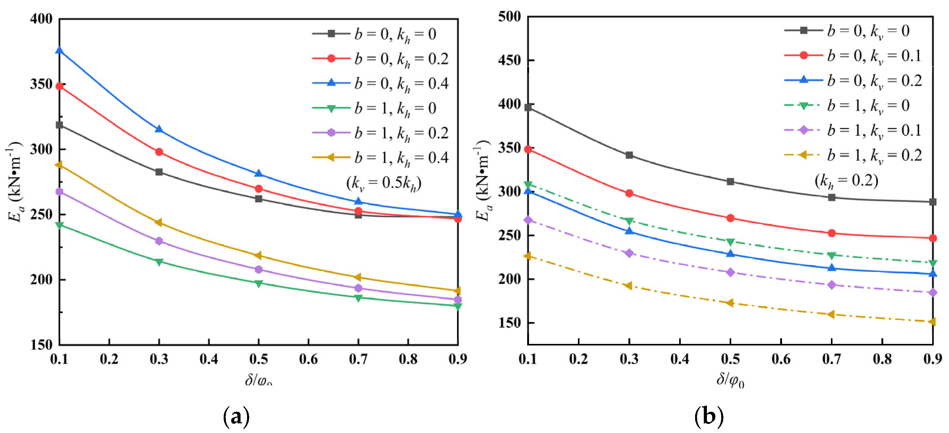
5.3. Active Earth Pressure Resultant Force
In this study, ; . The change curves of resultant force under different wall–soil friction angles and horizontal and vertical seismic coefficients are shown in Figure 8. It can be seen from Figure 8a that as and increased, gradually decreased. Under the same earthquake conditions, the resultant earth pressure of was lower than that of by 22.96%. On the contrary, increased as increased. However, with the increase of , this amplitude gradually decreased. When was close to the internal friction angle , the influence of on was no longer very obvious. In Figure 8b, had the same changing trend as , , and increased—that is, it gradually decreased in all cases.
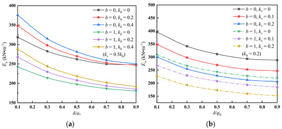
Figure 8.
Influence of and on : (a) and ; (b) and .
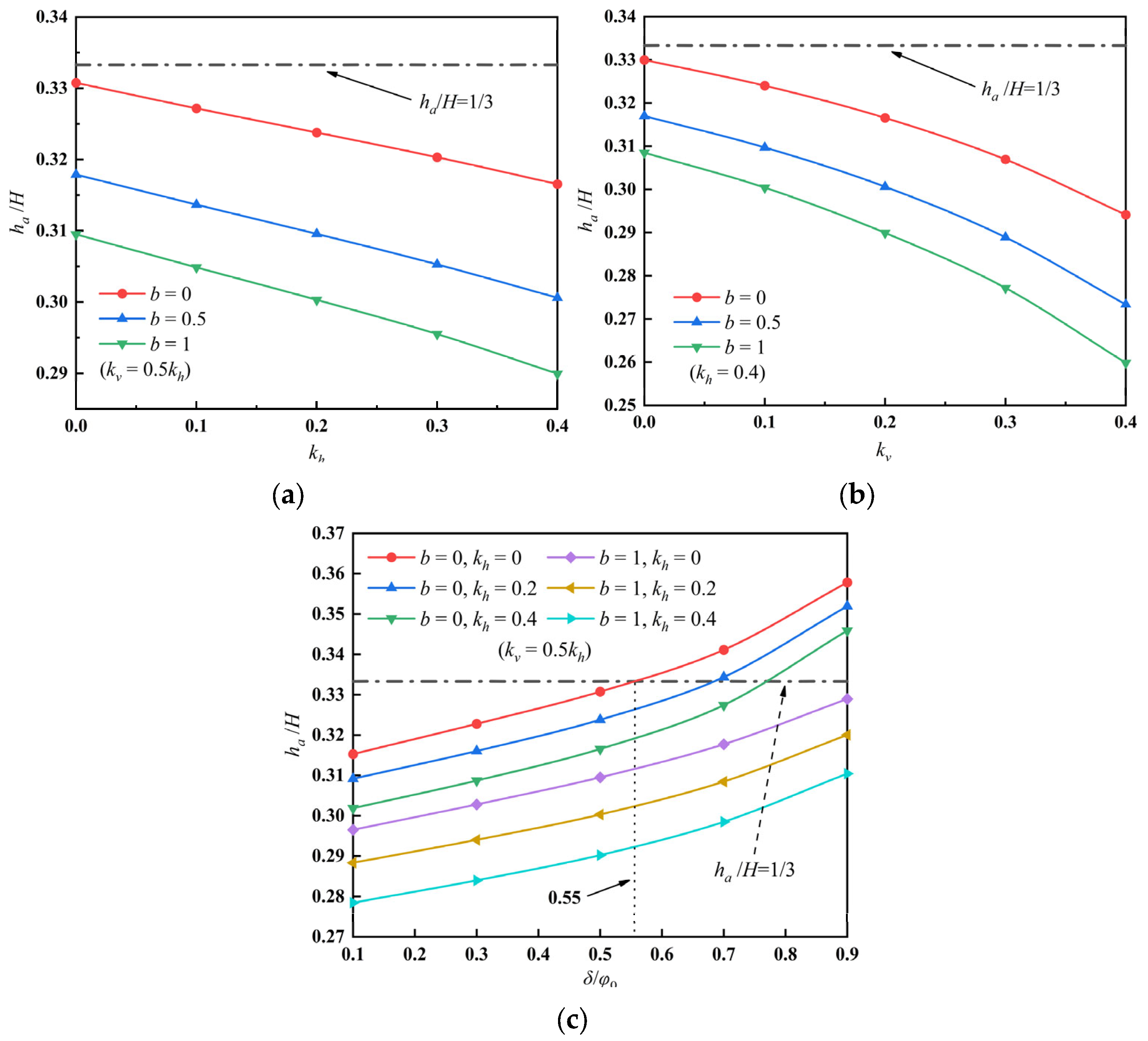
5.4. Resultant Force Action Point
We assumed that . The change curves of the resultant force action point under different horizontal and vertical seismic coefficients () and wall–soil friction angles () are shown in Figure 9. It is clear from Figure 9a,b that decreased with increasing , , and . The decreasing trend was approximately linear with increasing , while a nonlinear trend was observed for increasing . When , the initial reduction points of the two working conditions were located near the traditional earth pressure resultant point . In Figure 9c, unlike the seismic coefficient, gradually increased as increased. When was small, the resultant force action points under several working conditions were less than . However, when and , situations where the resultant force action points were greater than began to appear.
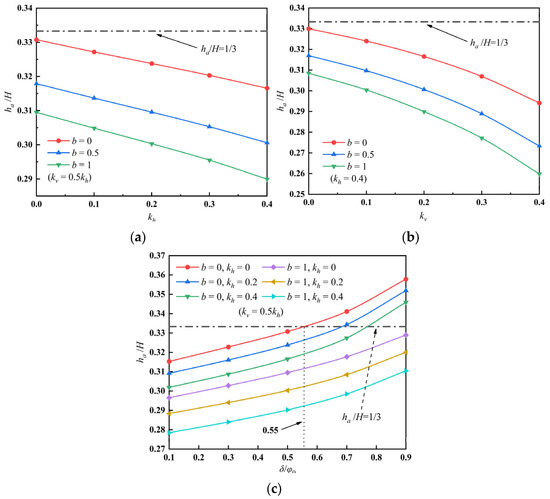
Figure 9.
Influence of , and on : (a) ; (b) ; (c) .
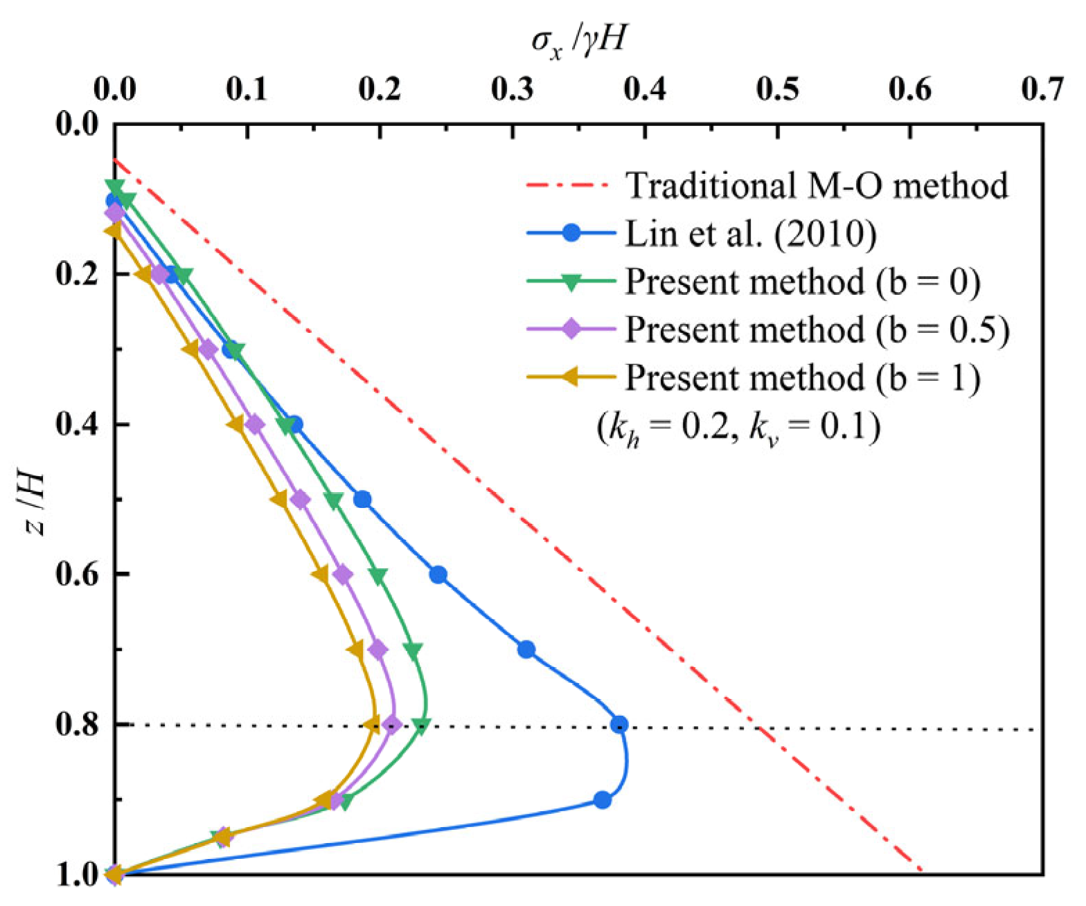
6. Comparison and Verification
In order to further illustrate the applicability of the method in this paper, the research results of Lin et al. [40] were selected for comparison. The relevant parameters were assumed to be: ; ; ; ; ; ; ; . The horizontal earth pressure distributions of several methods are shown in Figure 10. The traditional Mononobe–Okabe method leads to a linear distribution, while the results of Lin et al. [40] and the method in this paper both demonstrate nonlinear distributions. At the same time, based on the results of shaking-table tests of seismic earth pressure on retaining walls under different foundation conditions by Qu and Zhang [24], it is found that a “convex” nonlinear distribution in the lower part of the retaining structure is realistic. It can also be seen that the results obtained by the traditional Mononobe–Okabe method were much larger than the results of this paper and those of Lin et al. [40]. Compared with the results obtained by Lin et al. [40], the main gap was concentrated in the lower part of the retaining structure. This may be explained by the fact that the intermediate principal stress and soil arching effect were not considered, and because the linear slip surface was used simultaneously. However, both displayed the same trend, and the earth pressure reduction point was near , which is consistent with the previous analysis. This also shows that the method proposed in this paper is reasonable.
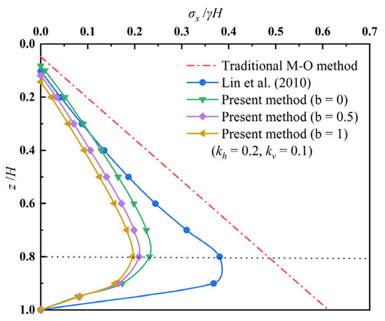
Figure 10.
Comparison of active earth pressure in previous studies.
7. Discussion
This study is the first attempt to apply the twin-shear unified strength theory to calculate the seismic active earth pressure under limited backfill. The influence of a curved slip surface is also considered, which has very important theoretical significance for the seismic earth pressure of limited backfill and the subsequent 3D earth pressure research. In the parameter sensitivity and comparative analysis, the earth pressure distribution form, the intermediate principal stress, the seismic coefficient, and the wall–soil friction angle were discussed.
The horizontal earth pressure presented a “convex” nonlinear distribution, which is consistent with the measured results obtained from the shaking-table test of a retaining structure by Qu and Zhang [24]. Lin et al. [40] also carried out theoretical research on seismic active earth pressure and obtained the same distribution form based on a semi-infinite space assumption. However, these previous studies did not comprehensively consider the effects of limited backfill width, intermediate principal stress, and soil arching effects. Therefore, there are still some obvious deviations between the results obtained in this research and previous studies, mainly in the middle and lower parts of the retaining structure. Nevertheless, the overall trend is consistent, and they are all different from the linear distribution of the classical Mononobe–Okabe theory [3,4] or a simple extension of it [22], indicating that the method proposed in this paper is reasonable. The seismic active earth pressure gradually decreased with the intermediate principal stress weight coefficient, by up to 22.96%. This indicates that the intermediate principal stress has a positive effect on further exerting the strength limit of the material, which presents good agreement with previous earth pressure studies considering the intermediate principal stress [32,33]. The lateral earth pressure coefficient deduced in this paper was affected by the vertical seismic coefficient . gradually decreased with , which is different from the research by Yang and Zhang [23] on the influence of the horizontal seismic coefficient on the earth pressure coefficient. The resultant force action point increased nonlinearly with the wall–soil friction angle , which also indirectly indicates that is significantly affected by the soil arching effects. It is worth noting that began to be greater than the classic resultant force action point when . The anti-overturning stability should be strengthened in retaining structure design.
It should be pointed out that the earth pressure is an approximate calculation. Regardless of which theory is adopted, there will still be a substantial difference between the theoretical value and the actual situation. In addition, the method proposed in this paper is a generalized model. From the perspective of safety, it assumes that the logarithmic spiral angle at the bottom of the retaining structure is , which makes the formula in this paper have certain limitations—that is, the critical width of the limited backfill under the curved slip surface cannot be given. At present, measurement data on the seismic earth pressure of soil with a limited width is very scarce. The formulas in this study need to be further verified and improved by many experiments in the future.
8. Conclusions
In soil with limited width, it is valuable to explore the action mechanism and distribution characteristics of active earth pressure under the action of intermediate principal stress and earthquake. Based on previous studies, the default slip surface is a logarithmic spiral. This study was carried out under complex conditions based on the plane strain twin-shear unified strength theory formula and considering the effects of soil arching and tension cracks. Three conclusions are summarized as below:
Due to the contribution of the intermediate principal stress, the lateral earth pressure coefficient, the horizontal active earth pressure, the resultant force, and the action point gradually decreased with the increase of the intermediate principal stress weight coefficient . When , the strength potential of the material could be increased by 22.96% at most under the same seismic conditions. Therefore, reasonable consideration of the influence of the intermediate principal stress can reduce the consumption of materials to a certain extent, which has considerable economic benefits in engineering.
The effect of earthquake on earth pressure is very significant. As the horizontal seismic coefficient increased, the active earth pressure and the resultant force gradually increased, while the action point gradually decreased. As the vertical seismic coefficient increased, the lateral earth pressure coefficient gradually decreased—when , the reduction of was the most obvious. In addition, as the wall–soil friction angle increased, the soil arching effects became increasingly obvious, gradually decreased, and gradually increased. It is worth noting that in the calculations in this paper, when and . At this time, it is necessary to strengthen the anti-overturning stability when designing retaining structures.
The pseudo-static method was used in this study to deal with the dynamic earth pressure under earthquake action when soil has a limited width, which is equivalent to a further improvement of the Mononobe–Okabe method. Through comparison with previous studies, we found that both methods presented a “convex” nonlinear distribution along the retaining structure, and the decreasing points were all near . This indicates that the method proposed in this paper is reasonable and can provide a new approach for the subsequent study of 3D seismic earth pressure considering the intermediate principal stress.
Author Contributions
Methodology, D.K. and H.L.; data curation, W.G. and B.W.; writing, H.L. All authors have read and agreed to the published version of the manuscript.
Funding
This research received no external funding.
Institutional Review Board Statement
Not applicable.
Informed Consent Statement
Not applicable.
Data Availability Statement
Data sharing not applicable.
Conflicts of Interest
The authors declare no conflict of interest.
References
- Rankine, W.J.M. On the stability of loose earth. Philos. Trans. R. Soc. 1857, 147, 9–27. [Google Scholar]
- Coulomb, A. Essai sur une Application des Règles de Maximis & Minimis à Quelques Problèmes de Statique Relatifs à L’architecture; De l’Imprimerie Royale: Paris, France, 1776; Volume 7, pp. 343–382. [Google Scholar]
- Okabe, S. General theory on earth pressure and seismic stability of retaining wall and dam. J. Jpn. Soc. Civ. Eng. 1924, 10, 1277–1323. [Google Scholar]
- Mononobe, N. Considerations into earthquake vibrations and vibration theorie. J. Jpn. Soc. Civ. Eng. 1924, 10, 1063–1094. [Google Scholar]
- Wang, Y.Z. Distribution of earth pressure on a retaining wall. Géotechnique 2000, 50, 83–88. [Google Scholar] [CrossRef]
- Zhang, H.B.; Liu, M.P.; Zhou, P.F.; Zhao, Z.Z.; Li, X.L.; Xu, X.B.; Song, X.G. Analysis of earth pressure variation for partial displacement of retaining wall. Appl. Sci. 2021, 11, 4152. [Google Scholar] [CrossRef]
- Hu, W.D.; Zhu, X.N.; Liu, X.H.; Zeng, Y.Q.; Zhou, X.Y. Active earth pressure against cantilever retaining wall adjacent to existing basement exterior wall. Int. J. Geomech. 2020, 20, 04020207. [Google Scholar]
- Frydman, S.; Keissar, I. Earth pressure on retaining walls near rock face. J. Geotech. Eng. 1987, 113, 586–599. [Google Scholar] [CrossRef]
- Liu, M.L.; Chen, X.S.; Hu, Z.Z.; Liu, S.Y. Active earth pressure of limited C-φ soil based on improved soil arching effect. Appl. Sci. 2020, 10, 3243. [Google Scholar] [CrossRef]
- Tang, Y.; Chen, J. A computational method of active earth pressure from finite soil body. Math. Probl. Eng. 2018, 2018, 9892376. [Google Scholar] [CrossRef] [Green Version]
- Xie, M.X.; Zheng, J.J.; Zhang, J.; Cui, L.; Miao, X. Active earth pressure on rigid retaining walls built near rock face. Int. J. Geomech. 2020, 20, 04020061. [Google Scholar] [CrossRef]
- Terzaghi, K. Theoretical Soil Mechanics; John Wiley & Sons: New York, NY, USA, 1943; pp. 66–76. [Google Scholar]
- Handy, L. The arch in soil arching. J. Geotech. Eng. 1985, 111, 302–318. [Google Scholar] [CrossRef]
- Take, W.A.; Valsangkar, A.J. Earth pressures on unyielding retaining walls of narrow backfill width. Can. Geotech. J. 2001, 38, 1220–1230. [Google Scholar] [CrossRef]
- Paik, K.H.; Salgado, R. Estimation of active earth pressure against rigid retaining walls considering arching effect. Géotechnique 2003, 53, 643–653. [Google Scholar] [CrossRef]
- Zhao, Q.; Zhu, J.M. Research on active earth pressure behind retaining wall adjacent to existing basements exterior wall considering soil arching effect. Rock Soil Mech. 2014, 35, 723–728. (In Chinese) [Google Scholar]
- Tsagareli, Z.V. Experimental investigation of the pressure of a loose medium on retaining walls with a vertical back face and horizontal backfill surface. Soil Mech. Found. Eng. 1965, 91, 197–200. [Google Scholar] [CrossRef]
- Ellis, H.B. Use of cycloidal arcs for estimating ditch safety. J. Soil Mech. Found. Div. 1973, 99, 165–197. [Google Scholar] [CrossRef]
- Yang, M.H.; Tang, X. Rigid retaining walls with narrow cohesionless backfills under various wall movement mode. Int. J. Geomech. 2017, 17, 04017098. [Google Scholar] [CrossRef]
- Yang, M.H.; Dai, X.B.; Zhao, M.H.; Luo, H. Calculation of active earth pressure for limited soils with curved sliding surface. Rock Soil Mech. 2017, 38, 2029–2035. (In Chinese) [Google Scholar]
- He, Z.M.; Liu, Z.F.; Liu, X.H.; Bian, H.B. Improved method for determining active earth pressure considering arching effect and actual slip surface. J. Cent. South Univ. 2020, 27, 2032–2042. [Google Scholar] [CrossRef]
- Iskander, M.; Chen, Z.B.; Omidvar, M.; Guzman, I.; Elsherif, O. Active static and seismic earth pressure for c-φ soil. Soils Found. 2013, 53, 639–652. [Google Scholar] [CrossRef] [Green Version]
- Yang, X.L.; Zhang, S. Seismic active earth pressure for soils with tension crack. Int. J. Geomech. 2019, 19, 06019009. [Google Scholar] [CrossRef]
- Qu, H.L.; Zhang, J.J. Shaking table tests on influence of site conditions on seismic earth pressures of retaining wall. Chin. J. Geotech. Eng. 2012, 34, 1227–1233. (In Chinese) [Google Scholar]
- Yang, X.L.; Chen, H. Seismic active earth pressure of unsaturated soils with a crack using pseudo-dynamic approach. Comput. Geotech. 2020, 125, 103684. [Google Scholar] [CrossRef]
- Li, Z.W.; Yang, X.L.; Li, Y.X. Active earth pressure coefficients based on a 3D rotational mechanism. Comput. Geotech. 2019, 112, 342–349. [Google Scholar] [CrossRef]
- Li, Z.W.; Yang, X.L. Analysis and design charts for 3D active earth pressure in cohesive soils with crack. Acta Geotech. 2020, 16, 1–15. [Google Scholar] [CrossRef]
- Yu, M.H. Twin shear stress yield criterion. Int. J. Mech. Sci. 1983, 25, 71–74. [Google Scholar] [CrossRef]
- Yu, M.H.; He, L.N.; Liu, Y. Generalized twin shear stress yield criterion and its generalization. Chin. Sci. Bull. 1992, 37, 2085–2089. [Google Scholar]
- Yu, M.H. Unified Strength Theory and Its Applications; Springer: Singapore, 2018; pp. 129–169. [Google Scholar]
- Zhang, J.; Hu, L.; Liu, H.B.; Wang, S.S. Calculation study of Rankine earth pressure based on unified strength theory. Chin. J. Rock Mech. Eng. 2010, 29, 3169–3175. (In Chinese) [Google Scholar]
- Jiao, Y.Y.; Zhang, Y.; Tan, F. Estimation of active earth pressure against rigid retaining walls considering soil arching effects and intermediate principal stress. Int. J. Geomech. 2020, 20, 04020217. [Google Scholar] [CrossRef]
- Shao, S.J.; Chen, F.; Deng, G.H. Seismic passive earth pressure against the retaining wall of structural loess based on plane strain unified strength formula. Rock Soil Mech. 2019, 40, 1255–1262. (In Chinese) [Google Scholar]
- Wang, K.H.; Ma, S.J.; Wu, W.B. Active earth pressure of cohesive soil backfill on retailing wall with curved sliding surface. J. Southwest Jiaotong Univ. 2011, 46, 732–738. (In Chinese) [Google Scholar]
- Ying, H.W.; Huang, D.; Xie, X.Y. Study of active earth pressure on retaining wall subject to translation mode considering lateral pressure on adjacent existing basement exterior wall. Chin. J. Rock Mech. Eng. 2011, 30, 2970–2978. (In Chinese) [Google Scholar]
- Goel, S.; Patra, N. Effect of arching on active earth pressure for rigid retaining walls considering translation mod. Int. J. Geomech. 2008, 8, 123–133. [Google Scholar] [CrossRef]
- Khosravi, M.H.; Kargar, A.; Amini, M. Active earth pressures for non-planar to planar slip surfaces considering soil arching. Int. J. Geotech. Eng. 2018, 14, 730–739. [Google Scholar] [CrossRef]
- Richards, R., Jr.; Elms, D.G.; Budhu, M. Dynamic fluidization of soil. J. Geotech. Geoenviron. 1990, 116, 740–759. [Google Scholar] [CrossRef]
- Ministry of Transport, People’s Republic of China. JTG B02-2013 Specification of Seismic Design for Highway Engineering; China Communications Press: Beijing, China, 2019. (In Chinese)
- Lin, Y.L.; Yang, G.L.; Zhao, L.H.; Zhong, Z. Horizontal slices analysis method for seismic earth pressure calculation. Chin. J. Rock Mech. Eng. 2010, 29, 2581–2591. (In Chinese) [Google Scholar]


Publisher’s Note: MDPI stays neutral with regard to jurisdictional claims in published maps and institutional affiliations. |
© 2021 by the authors. Licensee MDPI, Basel, Switzerland. This article is an open access article distributed under the terms and conditions of the Creative Commons Attribution (CC BY) license (https://creativecommons.org/licenses/by/4.0/).