TSCH Multiflow Scheduling with QoS Guarantees: A Comparison of SDN with Common Schedulers

Abstract

Industrial Wireless Sensor Networks (IWSN) are becoming increasingly popular in production environments due to their ease of deployment, low cost and energy efficiency. However, the complexity and accuracy demanded by these environments requires that IWSN implement quality of service mechanisms that allow them to operate with high determinism. For this reason, the IEEE 802.15.4e standard incorporates the Time Slotted Channel Hopping (TSCH) protocol which reduces interference and increases the reliability of transmissions. This standard does not specify how time resources are allocated in TSCH scheduling, leading to multiple scheduling solutions. Schedulers can be classified as autonomous, distributed and centralised. The first two have prevailed over the centralised ones because they do not require high signalling, along with the advantages of ease of deployment and high performance. However, the increased QoS requirements and the diversity of traffic flows that circulate through the network in today’s Industry 4.0 environment require strict, dynamic control to guarantee parameters such as delay, packet loss and deadline, independently for each flow. That cannot always be achieved with distributed or autonomous schedulers. For this reason, it is necessary to use centralised protocols with a disruptive approach, such as Software Defined Networks (SDN). In these, not only is the control of the MAC layer centralised, but all the decisions of the nodes that make up the network are configured by the controller based on a global vision of the topology and resources, which allows optimal decisions to be made. In this work, a comparative analysis is made through simulation and a testbed of the different schedulers to demonstrate the benefits of a fully centralized approach such as SDN. The results obtained show that with SDN it is possible to simplify the management of multiple flows, without the problems of centralised schedulers. SDN maintains the Packet Delivery Ratio (PDR) levels of other distributed solutions, but in addition, it achieves greater determinism with bounded end-to-end delays and Deadline Satisfaction Ratio (DSR) at the cost of increased power consumption.

1. Introduction

The adoption of Industrial Wireless Sensor Networks (IWSN) in industry requires devices and protocols that can guarantee physical operation and greater determinism in transmissions [1]. In order to satisfy the latency and reliability requirements of automation systems, even in converged environments, in which multiple information flows with different levels of priorities are involved. Therefore, the IEEE 802.15.4 standard, which specifies the physical and medium access control layers, has been updated to IEEE 802.15.4e. It maintains the physical layer, which consists of 16 channels in the 2.4 GHz band, and the medium access control replaces Carrier Sense Multiple Access with Collision Avoidance (CSMA/CA) with three new protocols [2] to support different types of industrially oriented applications. These are Low Latency Deterministic Network (LLDN), Deterministic and Synchronous Multi-channel Extension (DSME) and Time Slotted Channel Hopping (TSCH).

The protocols most adaptable to industry are DSME and TSCH, because they incorporate mechanisms to limit interference and increase determinism. They are based on time division to allocate transmission timeslots over different frequencies. However, the TSCH protocol is more widely used, because the slotframe it uses is simpler and has greater flexibility, as it allows the addition or removal of a single timeslot [3]. Because transmissions are made at a specific time, the transmitter and receiver must be synchronised, and they must be informed of the action to be taken at each instant of time. For this reason, a scheduling process is necessary to assign the transmission and reception timeslots as well as the channels on which they will be carried out. Currently, the standard does not define how to carry out this process, consequently, different proposals have emerged to generate TSCH scheduling.

These schedulers can be classified as centralised, distributed or autonomous, depending on the entity that makes the decision to allocate the slots. In the centralised ones, a central element, called Path Computation Element (PCE) is in charge of assigning the scheduling to each node. Among the most representative of these are the Traffic Aware Scheduling Algorithm (TASA) [4] and Adaptive Multihop Scheduling (AMUS) [5]. In distributed scheduling, nodes negotiate with their neighbours to allocate slots. Among these are Decentralized Traffic Aware Scheduling (DeTAS) [6] and Wave [7]. Finally, the autonomous ones reuse information from other protocols and each node assigns its scheduling locally. Among these is Orchestra [8], along with certain variants such as Escalator [9] and Autonomous Link-based Cell scheduling (ALICE) [10].

Centralised schedulers allow more complete control of transmissions, as the PCE does the scheduling with full knowledge of the topology. However, the additional traffic between the nodes and the PCE decreases the available bandwidth at each node. This has led to the widespread use of autonomous and distributed solutions, which do not require this additional load of control traffic. One of the most widely used autonomous schedulers is Orchestra, due to its reliability, high performance and availability by default in the Contiki-NG (https://www.contiki-ng.org/, accessed on 15 November 2021) operating system. In accordance with [8], this protocol achieves a packet delivery ratio of 99.9%. However, the constant increase in QoS requirements requires that other parameters such as end-to-end delay and deadline, be guaranteed in order for IWSN to adapt to the convergence of flows of different priorities. Satisfying these requirements with autonomous or distributed schedulers means increasing the complexity of the protocols, as their local operation results in sub-optimal solutions.

For these reasons centralised schedulers are necessary. However, to compensate for the limitations they present, a disruptive approach such as Software Defined Networks (SDN) is needed. In contrast to centralised scheduling solutions that only have control over the MAC layer, an SDN solution allows control over all layers, which makes it possible to manage all decisions and processes that take place at the nodes. Hence, with this type of scheduler it is possible to meet the increased QoS requirements.

However, SDN integration is not straightforward, due to the difficulty of managing control traffic in a resource-constrained environment. This has led to multiple implementations such as SD-WSN [11], TinySDN [12], Atomic SDN [13] and SDN-WISE [14]. However, these solutions use the CSMA protocol as MAC, which makes them unfeasible in industrial environments with deterministic requirements. To adapt to these environments, it is necessary to have solutions that use the TSCH protocol such as Whisper [15], uSDN [16] and SDN WISE-TSCH [17]. Whisper and uSDN are based on a traditional TSCH RPL network using the 6TiSCH protocol stack, where in the case of Whisper the SDN controller injects “fake” messages that modify the metrics of the nodes in order to alter the operation of the routing and schedulling protocols, whereas uSDN injects configurations through the Constrained Application Protocol (COAP). However, in both cases the use of standardized upper layers limits the flexibility of software-defined networking. In the case of SDN WISE-TSCH extends the performance of SDN WISE that offers a complete design of all layers and protocols to allow full centralised management, therefore all layers and protocols are optimised to minimise control traffic. Because of this it has less control traffic than AMUS but still more than Orchestra. However, the control that is obtained over the entire network means that the adverse effects of this type of traffic are avoided [17].

This paper focuses on analysing the advantages of software defined networks to guarantee strict QoS parameters in multi-flow environments. Different scenarios with industrial level characteristics are simulated using different TSCH schedulers that are available and have been extensively studied [18,19,20]. Performance is evaluated in terms of end-to-end delay, packet delivery ratio, deadline satisfaction ratio and power consumption. In addition, a testbed is implemented to compare the two protocols that have shown the best performance in the simulations, evaluating the end-to-end delay and the Packet Inter-Arrival Time (PIAT).

The rest of the paper is organised as follows. Section 1 introduces the TSCH and Routing Protocol for Low-Power and Lossy Networks (RPL) and the different scheduling protocols. Section 2 presents a description of the scenario and the metrics used in the tests. Section 3 contains the simulation results for each of the metrics, and the testbed results. Discussion and conclusions are shown in Section 4.

1.1. RPL and Time Slotted Channel Hopping

RPL is the standard routing protocol designed for Low-power and Lossy networks (LLN) devices, which have limitations in power processing, memory and energy consumption. According to the standard [21] this protocol represents the topology of routing through Destination-Oriented Directed Acyclic Graph (DODAG) oriented towards the root node or sink and is also the protocol used to build the topology in a WSN. To build it, it is necessary to exchange control messages, called DODAG Information Objects (DIO) and Destination Advertisement Object (DAO), which each node sends continuously. These messages contain information about the routing metric and the objective function to be used to find the parent node, which according to the objective function will be the optimal path to reach the root.

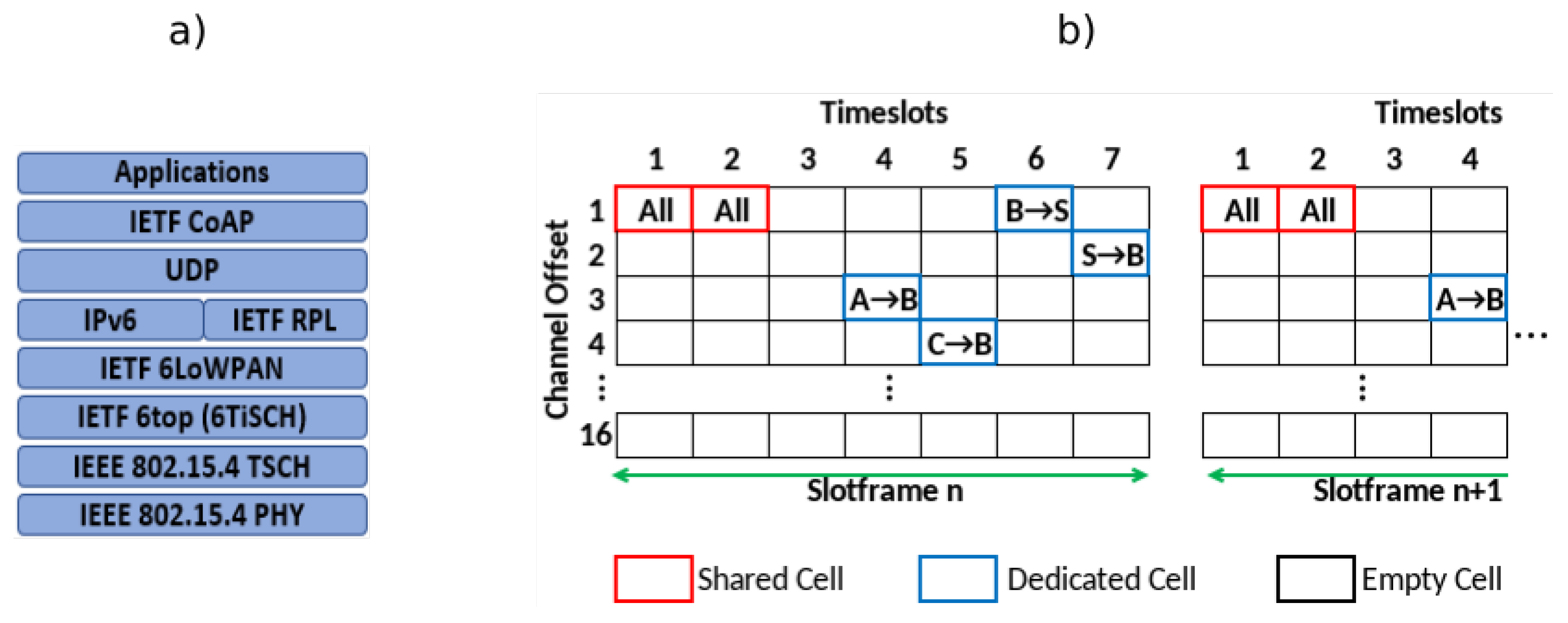
The RPL process starts when the DODAG root node sends a DIO message with a range equal to 1. When it is received, the nodes update their range, which will be the distance to the root node. In addition, they use the objective function to select the best path to the root. This protocol is part of the 6TiSCH stack Figure 1a, which includes the necessary protocols to adapt IPv6 to industry standards.

The TSCH media access control protocol, is defined in the standard IEEE 802.15.4e, and is considered a suitable solution for providing real-time multi-hop transmissions in industrial environments [22]. TSCH offers guarantees in terms of latency and data delivery in IWSNs since it allows nodes to have a guaranteed space to send their packets. To do this, it divides the time into a fixed number of timeslots which are grouped into slotframes, which are cyclical, see Figure 1b. The most common duration of each timeslot is 10 ms, enough time to be able to transmit a frame of the maximum size (127 Bytes), to wait for the Acknowledgement (ACK) from the receiver, and to process the packet. The frequency division is done with the assignment of a channel offset, which is used to determine the physical channel, therefore a timeslot and a channel offset must be defined for each transmission. The combination of these two parameters is a cell, which can be shared or dedicated. In the case of shared, any of the nodes can transmit if they have packets to send, otherwise the node goes to receiving mode.

Therefore, in the shared slot the CSMA scheme is followed with backoff exponent to reduce collisions. On the other hand, if it is dedicated, a uni-directional link is established between two nodes and only the source node can transmit during the timeslot and in the specific offset channel. This time division requires that all nodes are synchronised so that they can exchange information. This is achieved with the Enhanced Beacon (EB) packet exchange, which includes information about the Absolute Sequence Number (ASN) which the nodes take as a time reference and determines the current timeslot. It also allows the clock drifts to be compensated. The ASN information is used with Channel offset to generate a rotation of the physical channels in each slotframe using Equation (1). This helps reduce the points of interference and path fading, thus increasing reliability.

$$frequency=F\left[(ASN+C{h}_{offset})mod{N}_{ch}\right]$$

(1)

To allocate each of the cells in the nodes, there must be a scheduling process to synchronise the transmission and reception states. However, the IEEE 802.15.4e standard does not include any specification on how to do this. For this reason, the following section explains different types of schedulers and details the operation of the most common of these.

1.2. TSCH Schedulers and Protocols

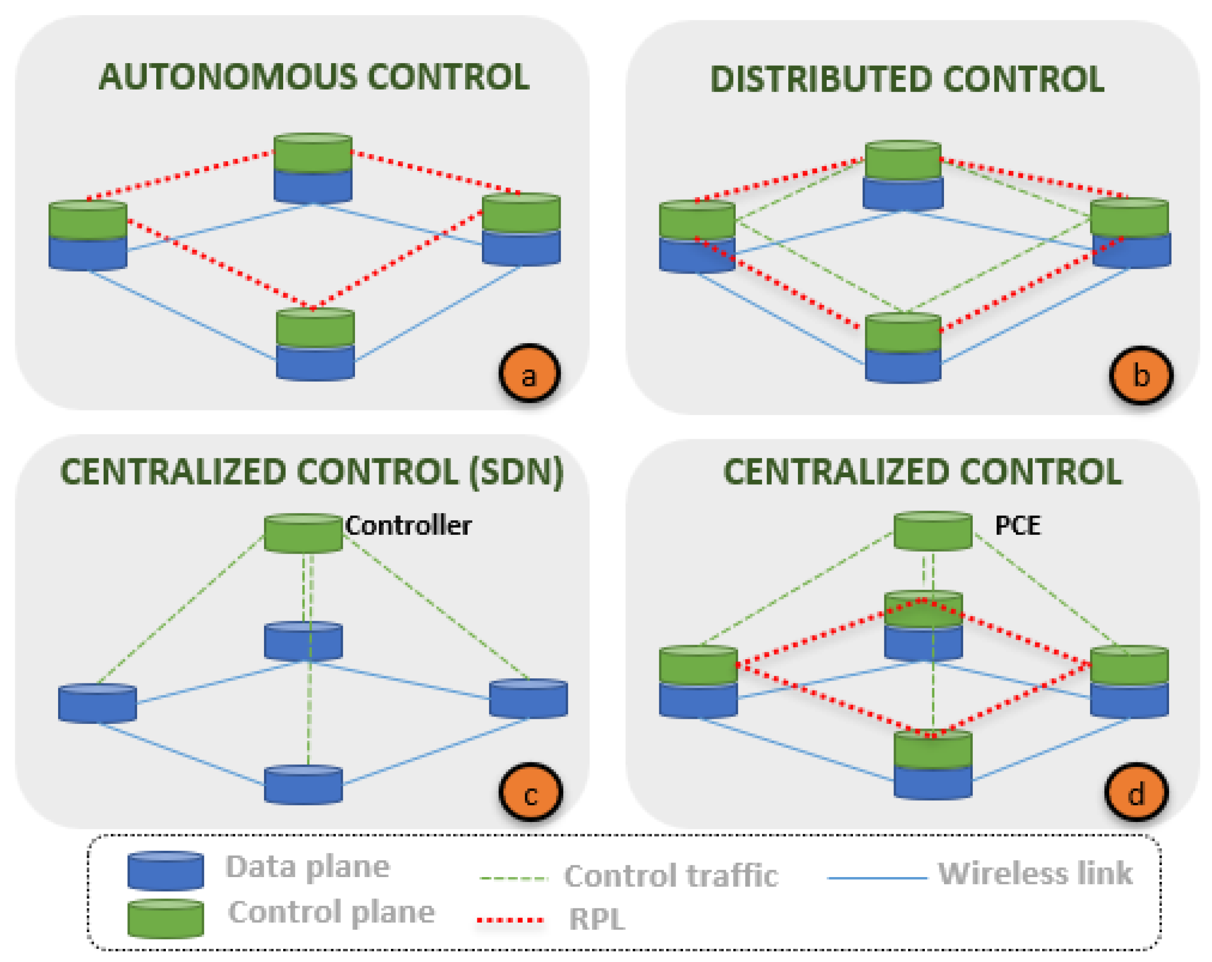
To assign the operating states of each node to the corresponding cells, it is first necessary to carry out the TSCH scheduling process. This decides what action the node will perform in each timeslot. The node will be able to receive, transmit, or sleep. The nodes covered by the scheduler must be correctly synchronised so that the transmission and reception timeslots match. Because there is no standard for this scheduling, multiple TSCH schedulers have been developed, which can be classified into autonomous, distributed and centralised. In addition, SDN is considered a more specialised centralised approach which separates the control plane and the data plane to optimise the overall performance.

The differences between each of the approaches can be seen in Figure 2, using the same topology. In Figure 2a autonomous scheduler, the nodes only exchange RPL messages over established wireless links, and each node reuses the obtained RPL information to do the scheduling. In distributed schedulers Figure 2b, in addition to the RPL information, the nodes exchange negotiation packets to request or accept cells in the TSCH schedule. In centralised Figure 2c,d a single device is used to create the scheduling, therefore each device must send control traffic with topology information. However, the simple centralised Figure 2d, maintains the operation of the devices and protocols as in Figure 2a,b. In Figure 2c, the devices and protocols are simpler since they do not have to make any decisions because the control plane is completely centralised. This section briefly describes the main features of the existing TSCH schedulers, as well as the specific performance of some of them which will be used in a comparative analysis.

1.2.1. Autonomous

One of the characteristics of autonomous TSCH schedulers is that they reuse the topology and routing information stored by the nodes to perform the scheduling. This information is obtained through the exchange of RPL control messages with their neighbours, Figure 2a. Therefore, no additional signalling is required for the formation of the different schedules and only the MAC address and updated topology information is needed. The most commonly used autonomous scheduler is Orchestra [5], due to its ease of configuration and high performance.

In Orchestra, each node creates and maintains its own TSCH scheduling and updates it as changes occur in the network. In fact, they only use the RPL information received from neighbours and parents. An Orchestra schedule is composed of several Slotframes, each for a different type of traffic: Beacon messages (broadcast), RPL messages or Unicast messages (application traffic).

Four types of slots are defined in Orchestra:

• Common Shared Slot (CS): a common cell in all the nodes used for transmission and/or reception.
• Receiver-based Slot (RBS): there is one cell in reception and one cell in transmission for each neighbouring node, the position of the cell is calculated with the information from the Receiver.
• Sender-based Slot (SBS): there is one slot in transmission for each node and one in reception for the neighbours. The difference with the previous one is that the position of the cell is calculated with the information of the Sender.
• Sender-based Dedicated Orchestra Slots (SBD): this is a specific transmission slot for each neighbour, but in this case instead of using shared cells, a dedicated cell is used.

On the other hand, the different slotframes that can make up the scheduling with Orchestra are:

• EB Slotframe: this is a slotframe consisting of dedicated Sender-based Slots, and is for the transmission of EB messages.
• Broadcast Slotframe: this is a slotframe consisting of Common Shared Slots (shared cells), mainly for RPL traffic.
• Receiver-based Unicast Slotframe: for unicast traffic consisting of Receiver-based cells.
• Sender-based Unicast Slotframe: for unicast traffic consisting of Sender-based cells.

Orchestra scheduling can be carried out in two different configurations, Receiver-based or Sender-based:

(a)

Configuration Receiver-based: this consists of an EB Slotframe, a Broadcast Slotframe and Receiver-based Unicast Slotframe.

(b)

Configuration Sender-based: this consists of an EB Slotframe, a Broadcast Slotframe and a Sender-based Unicast Slotframe.

1.2.2. Distributed

These schedulers are based on negotiating the cell allocation of each node with its neighbours. In terms of reliability and delay performance they are similar to autonomous schedulers. They are also based on the RPL protocol, but have an added cost for the signalling and control messages used in the negotiation, Figure 2b. In [23], three possible alternatives are considered for the allocation of a cell from one node to an adjacent node: sharing of the same cell between all nodes, which reduces the complexity of signalling schedules but has negative effects in larger networks due to possible interference. Secondly, negotiation of a timeslot, which leads to an increase in energy consumption due to the exchange of messages. In addition, the last option, an arbitrary timeslot, which requires the use of hash functions to calculate the cell coordinates to be assigned by two adjacent nodes.

The choice of allocation strategy will be determined by the requirements of the application in use. For an application with reliability requirements and high traffic load, the additional signalling option shall be chosen, whereas if there are more timing requirements, the use of hash functions is recommended. Decentralized Traffic Aware Scheduling (DeTAS) [6], Wave [7] and 6TiSCH Minimal Scheduling Function (MSF) [24] are some of these distributed schedulers. However, hybrid algorithms using both strategies (hash and control messages) have also been proposed, such as DIS-TSCH [25].

MSF defines how the scheduling of communications is managed in a distributed manner. It is built on the simplest scheduling scheme, scheduling with TSCH minimal. In this case, the scheduling is stored in the node, so there are no processes for cell allocation. Together with Orchestra, it is also the default in the Contiki-NG operating system. It contains a single slotframe with a preconfigured length where a single cell is scheduled for all nodes.

In this way, any type of traffic is sent using this cell (EB, Data, RPL) [26]. As all nodes transmit and receive in the same timeslot and on the same channel Offset, this is called a shared cell, where collisions are very likely to occur. This single-slot operation results in very low energy consumption at the expense of a higher number of queued packets due to retransmissions. To improve performance, MSF includes a range of features that allow it to negotiate cells.

Once a node has successfully joined and synchronised to the network, it can add, remove or relocate cells if any of the following reasons exist:

• Adapt the link layer resources to the traffic between the node and the parent.
• Topology changes or parent switching.
• Managing a collision in the scheduling.

1.2.3. Centralised

Unlike the previous solutions where the nodes build their topology, in the centralised ones an external element known as PCE performs the cell allocation process of the entire network and sends this scheduling to the nodes. For this, the PCE collects topology information from specific messages created by each node. These messages contain the adjacent nodes and transmission statistics. This centralisation allows schedules with a high level of optimisation to be built, making them ideal for time-critical applications, as they can guarantee low latencies. This is the case for schedulers such as TASA [4], AMUS [5] and SDN WISE-TSCH [17]. The main problem with this approach is the traffic generated between the PCE and the nodes, which has a significant impact on network bandwidth.

AMUS [5] is a TSCH scheduling protocol that provides reliability in terms of achieving low latency for applications with low latency requirements, as is the case with most industrial applications and processes. It has outperformed TASA [4], the centralised default protocol. In comparison AMUS performs better in terms of reliability and delays. Although AMUS is not available, the paper [5] contains a detailed explanation that has allowed it to be used in the comparison.

This method is based on the reservation of the different scheduling cells (resources) along the different routes followed by the packets in a network. In this sense, the algorithm achieves this goal through a process consisting of three phases:

(a) Collecting information from the network. Using routing and control protocols, such as RPL, network statistics information is collected in order to know parameters such as the number of packets generated by a node in a period, topologies, etc.

(b) Cell assignment. For correct scheduling without collisions and with time guarantees, it is necessary to know in advance the sending sequences that are going to be carried out. This is because the nodes closest to the sink must route packets from nodes that are further away. Therefore, the cell in charge of transmitting the packets to the sink must be located in a timeslot after the reception of the packet to be transmitted. The process to be followed is as follows:

• Knowledge of the routes that the packets of each traffic flow will take to the sink.
• Construction of the Scheduling Sequence (SS) matrix: this is a 2·n (n = number of nodes that transmit packets) matrix, where the first row indicates the ID of the transmitting node and the second row indicates the traffic rate of each node. Each column of the SS matrix represents a traffic flow.
• Construction of the Multi-hop Scheduling Sequence (MSS) matrix: this is a matrix composed of three rows, the first being the source node, the second the destination node and the third the traffic rate. Each column of the matrix represents a link between two adjacent nodes.
• Scheduling: once the MSS matrix is obtained, the cells are assigned in column order, starting from the first free timeslot and the first Channel Offset. As many cells shall be assigned as indicated by the rate (third row).

Cells should be allocated according to the following restrictions, to avoid collisions or interference:

• Nodes can only have one state per timeslot (transmission or reception).
• Transmissions from other links that may cause collisions or interference should be made on another channel of the same timeslot.
• Links that do not have any conflict or interference can be allocated in parallel. In this case the same timeslot can be used.

SDN WISE-TSCH is a highly deterministic system that guarantees industrial level requirements. It has a stack of protocols that allow centralised control of all processes in the nodes (MAC, Routing, QoS, Application). This is based on the SDN paradigm, which consists of managing networks by separating the control plane and the data plane [27]. The control plane is entirely software-controlled, where a centralised agent, in this case a controller, makes decisions to configure resources and rules in the nodes. The data or forwarding plane are made up of the nodes, which operate in plug and play mode, as it is the controller that sends each node all the necessary instructions to achieve maximum performance.

As with all centralised schedulers, in SDN WISE-TSCH [17] message exchange between the nodes and the controller is required. However, as the whole protocol stack is designed for SDN, the topology discovery is optimised, so it does not require the use of the RPL protocol as shown in Figure 2c. For this reason, the control traffic is less than that used by AMUS, which in addition to communication with the controller, requires the use of RPL as shown in Figure 2d. The topology is managed through the following applications:

• Traffic Manager: This contains the specifications of the different traffic flows, which are classified by priority, deadline, source and destination node.
• Routing process: It is responsible for creating the source and destination routes for each flow. It uses as metrics the RSSI and the congestion level of each node which are updated each time a route is assigned.
• TSCH Scheduler: For each route it allocates the corresponding TSCH resources, generating schedules that guarantee a minimum end-to-end delay and deadline for each flow.

The integration of these three applications allows network slicing, which consists of the differentiation, isolation and logical segmentation of data flows, by means of the allocation of TSCH resources. This slicing makes it possible to guarantee QoS parameters for each data flow independently.

The scheduling algorithm is composed of multiple matrices, which are responsible for storing the information of the allocated cells. In this case there are two matrices of the same dimension as the slotframe, one storing all transmitting nodes and one for receiving nodes. It uses the same constraints as AMUS to avoid collisions and interference. In addition, the hops are allocated consecutively, in order to obtain the shortest delay. It also uses the deadline to adapt the flows to the length of the slotframe. For this, repetitions are used, which consist of allocating the resources of the route in different positions of the slotframe. This guarantees the specific bandwidth for each flow and decreases latencies independently of the slotframe length. The steps performed by the algorithm are as follows:

• Organize the traffic manager flow table by priority and deadline.
• Calculate the routes for each of the flow table entries.
• For each of the routes, perform a hop decomposition.
• Calculate the number of iterations to install over this route, according to the length of the slotframe/deadline.
• Perform cell assignment for each hop, where a conflict-free timeslot is sought, i.e., to search in the two matrices for a column where the transmitting and receiving node have no assigned states.
• Shifts the next iteration of the route by number of timeslots equal to the deadline and repeats the cell allocation process.

To increase flexibility and reduce the number of control packets, the sending of the scheduling is done by flows. This allows transmission of a single packet from the controller to configure a complete route from source to destination. This packet includes the routing and TSCH information. In addition, due to the integrated operation, these processes contain information on the type of traffic to be sent along this route, which allows allocation of dedicated resources for each type of traffic.

The main features of each TSCH scheduler are summarised in the

Table 1. Summary of features for each of the TSCH schedulers.

	SDN WISE-TSCH	AMUS	MSF	ORCHESTRA
Topology construction	SDN WISE: Beacon and Report	RPL	RPL	RPL
Scheduling distribution	Centralised	Centralised	Distributed	Autonomous
Resource reservation	Dynamic and specific according to deadline and data rate	Specific according data rate	One single shared cell negotiated cells	One single unicast cell
Response to changes	Yes Dynamic configuration and load balance	No. Pre-scheduling	Yes (RPL messages)	Yes (RPL messages)
Avoid collisions	Yes	Yes	No	Yes
Traffic classification	Yes all traffic can be marked, classified and special rules can be applied for each type.	No.	No	Only: Broadcast (RPL message), EB (Beacon), Unicast

.

2. Materials and Methods

The Cooja simulator, available as part of the Contiki-NG operating system, was used to analyse the performance of the described schedulers using Multi-Path Ray-tracer Medium (MRM) $n=2.04$ and $\sigma =6.7$. The hardware used for simulation is a intel core i7 with 16 GB of RAM and the nodes are modeled as OpenMote nodes. The payload used is 110 bytes, because the maximum packet size of the 802.15.4 standard is 127 bytes, of which 17 are used for the MAC header.

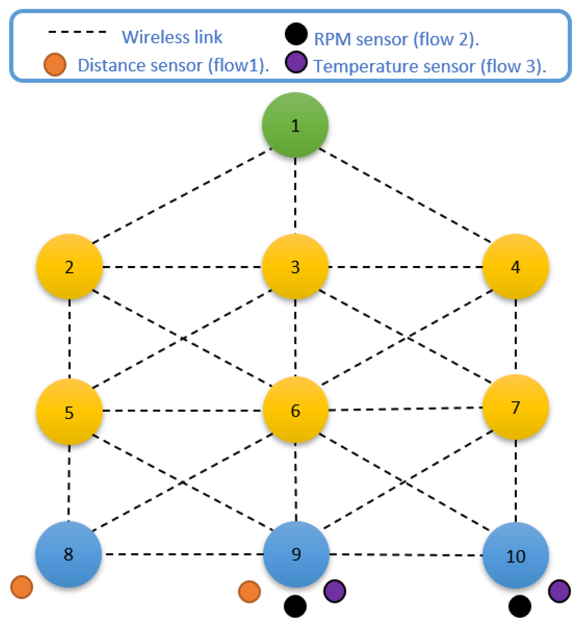
A network with a mesh topology typical in the industrial sector was used, because it offers higher reliability as it can route data through multiple paths [28]. The topology is shown in Figure 3. It is composed of 1 sink node, 6 relay nodes and 3 nodes (8, 9, 10) which will introduce traffic flows to the network with different quality of service requirements.

To characterise the flows, the reliability and latency requirements, typical of industrial systems, as defined in IEC 62264 (ANSI/ISA95), have been used. According to this standard, the 3 data flows used are:

• Supervisory Control Job Based: Latency less than 100 ms, loss less than ${10}^{-6}$ and number of devices less than 10.
• Supervisory Control Flow Based: Latency less than 100 ms, loss less than ${10}^{-7}$ and a number of devices less than 30.
• Monitoring: Latency of less than 1 s, a loss of less than ${10}^{-5}$ and a device count of less than 10,000.

As shown in Figure 3 the flows have a different packet period: 70 ms (flow 1, type supervisory control), 140 ms (flow 2, type monitoring) and 500 ms (flow 3, type monitoring) respectively.

In the simulation, two tests were carried out. Test 1 consisted of observing the behaviour of the network with low saturation, using monitoring and supervisory control flows. In this case node 9 would independently send each of the flows to the sink node. The following measurements were obtained for each of the packet periods:

• End-to-End Delay: milliseconds that elapse from the time a packet is generated at the transmitting node and its arrival at the destination. It is measured for each packet received.
• Packet Delivery Ratio (PDR): ratio of the number of packets sent and received by the destination node.
• Radio Duty Cycle (RDC): percentage of time the radio remains on in the transmit or receive state.
• Packet Inter-Arrival Time (PIAT): is the number of milliseconds that elapse between each reception of the same type of packet at the destination node. This metric allows evaluation of how well the network adapts to the strict time requirements.
• Deadline Satisfaction Ratio (DSR): this metric is obtained from the PIAT, and is the cumulative percentage of packets that remain below the deadline.

In test 2, a multi-flow test was performed to evaluate the behaviour in a network with more traffic. For this purpose, supervisory control and monitoring type flows have been used together. In this case nodes 8, 9 and 10 transmitted all the flows assigned simultaneously to node 1, which acts as sink. The packet inter-arrival time were then observed. This allows us to know the behaviour of the node with flows of different priorities typical in the industrial sector.

In TSCH the bandwidth depends on the amount of transmission timeslots in each slotframe, therefore, a lower number of timeslots in the slotframe increases the bandwidth. Since Orchestra and MSF by default send one packet per slotframe, a length of 7 timeslots will be used, as this is the minimum length configurable for the number of nodes without Orchestra over-allocating the cells. This slotframe size allows a higher bandwidth to adapt to the flow with the packet period of 70 ms. The parameters used in the simulations are summarised in

Table 2. Simulation parameters.

Parameter	Value	Units
Radio Medium	MRM ($n=2.04$, $\sigma =6.7$)
Timeslot	10	ms
# Channels	4	channels
EB Period	16	s
Slotframe Length	7	timeslots
# Packets	500	packets
Packet Period	70, 140, 500	ms
Packet Payload	110	Bytes
Max retransmissions	10	retransmissions

.

3. Results

This section includes the results of the simulation of the four TSCH scheduling methods, for each of the proposed metrics. In test 1 the end-to-end delay and packet delivery ratio (Section 3.1), radio duty cycle (Section 3.2), packet inter-arrival time and deadline satisfaction ratio (Section 3.3) have been evaluated. Test 2 includes the multi-flow tests (Section 3.4).

3.1. End-to-End Delay and Packet Delivery Ratio

The size of the queues in each scheduler is directly related to the end-to-end delays and the PDR, since it is the number of packets waiting to be sent. The default capacity is 8 packets, which in this case is the one used by SDN WISE-TSCH and AMUS. For Orchestra and MSF a capacity of 64 packets is used. This queue capacity reduces the memory available to each node, therefore, schedulers that require less memory usage are more efficient.

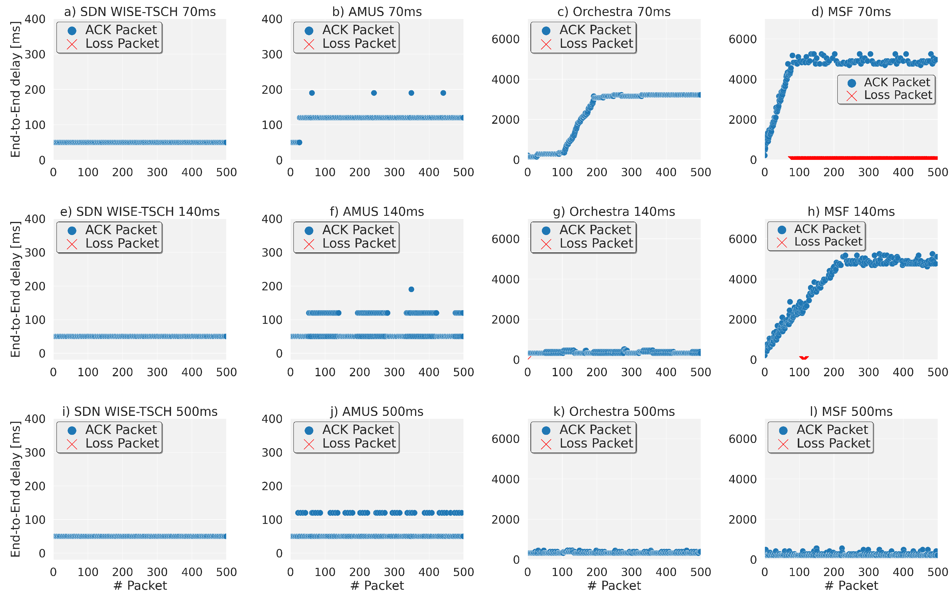
Figure 4, shows the end-to-end delay for the first 500 packets where there is already a stable operation that allows us to clearly observe the behaviour of each scheduler. Because the centralised schedulers achieve in all cases a lower end-to-end delay, a different scale has been used in Figure 4a,b,e,f,i,j which allows the differences between these schedulers to be observed.

The transmissions of each flow are performed independently, from the source at node 9, to the sink at node 1, for the four types of schedulers. In Figure 4a–d, a packet is sent every 70 ms. The centralised schedulers, such as SDN WISE-TSCH and AMUS, achieve the lowest delay, 50 ms for SDN WISE-TSCH and for AMUS a variation between 50 ms and 120 ms. The AMUS changes are due to the control traffic that accumulates in the same queue as the data flow, and in this case the queue is never more than 2 packets. However, with Orchestra there is an average delay of 2300 ms, due to the fact, that by default, Orchestra only allocates one unicast transmission slot in each slotframe. Therefore, this sending period (70 ms) is the maximum that Orchestra can have with a slotframe length of 7 timeslots. Because it must also send RPL control packets, there is an accumulation of packets in the queues, which is observed as a progressive rise from the 100th packet. In this case the queues reach a size of up to 40 packets, which causes an increase in the end-to-end delays. The most critical case is that of the MSF, which has the same drawback as Orchestra: 1 transmission slot per slotframe. In addition, at the beginning of transmissions, a timeslot shared with other nodes is used, which causes collisions. As retransmissions are enabled, the number of packets in queue grows faster than in Orchestra, as colliding packets accumulate, resulting in long delays and a large number of (network) losses.

Increasing the sending period to 140 ms results in the graphs Figure 4e,f, which shows that for the centralised schedulers there is no variation and the 50 ms for SDN WISE-TSCH and the 50 ms to 120 ms for AMUS are still maintained. In Figure 4g for Orchestra, a more stable behaviour is observed because there are fewer packets in queue, as seen in Figure 4h, where a clear improvement in packet loss and end-to-end delay is observed, since a higher available bandwidth allows unicast cells with the other nodes to be negotiated with the other nodes.

For a 500 ms period, there are no significant changes in the centralised schedulers Figure 4i SDN and Figure 4j AMUS. Orchestra in Figure 4k improves due to fewer packets in queue and its average end-to-end delay is 330 ms. In Figure 4l MSF has no more losses and the average delay of 230 ms is lower than Orchestra’s, since with a less saturated network the shared slots have a lower probability of collisions and allow traffic to be sent from the unicast queues.

Unlike the delay, which is different for each of the schedulers, the packet delivery ratio is close to 100% in most cases. This is because SDN WISE-TSCH and AMUS have configured the number of timeslots needed to send all the traffic they generate, which prevents buffer overflow. Orchestra has a PDR of 100% because it uses larger capacity buffers, which avoids packet loss since they are stored even if this means increasing the end-to-end delay. However, MSF is the only one that presents significant losses in the proposed scenario due to the use of shared slots that produce collisions. Only in cases of low saturation does MSF manage to increase the PDR close to 100%.

3.2. Radio Duty Cycle

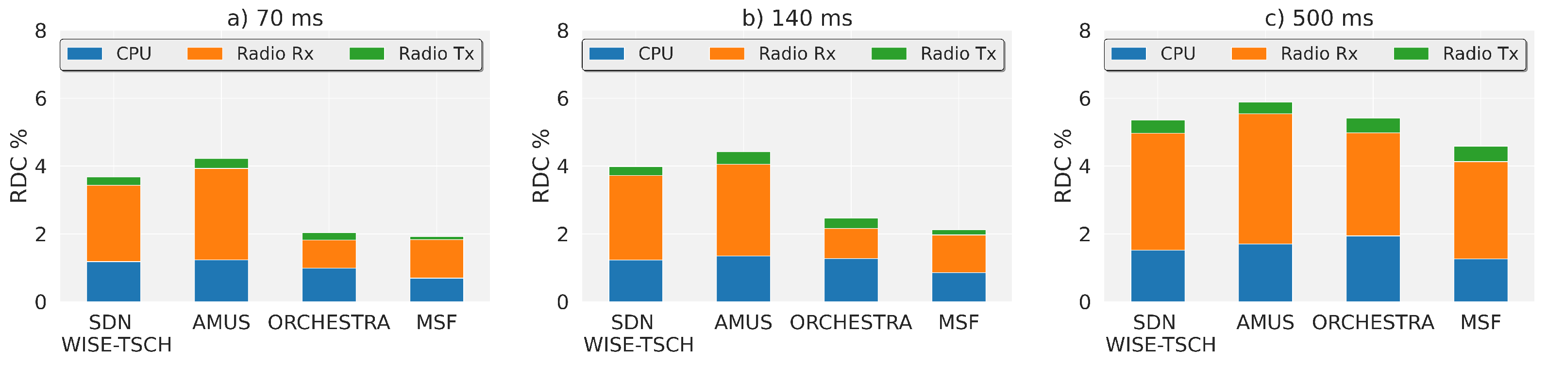
The energy consumption in TSCH is mainly due to radio use and can be estimated as the fraction of time that each node remains in the transmit and receive states. Therefore, the use of different scheduling processes causes a large variation in power consumption over the same scenario. In Figure 5a the different schedulers are observed with a packet period of 70 ms. MSF has the lowest consumption, which is due to the use of a shared slot and the dynamic allocation of the dedicated slots. Orchestra has a slightly higher consumption with a higher use of the radio in transmission due to the fact that in addition to the shared slot, it has a dedicated transmission slot in each node. For SDN WISE-TSCH and AMUS, the same amount of transmit and receive states are used. The difference in consumption is due to the amount of control traffic sent by each. SDN WISE-TSCH uses a proprietary protocol to exchange messages with the controller with less impact on bandwidth. AMUS uses the RPL protocol in addition to the communication with the PCE.

Increasing the packet period to 140 ms slightly increases the radio usage in all protocols Figure 5b, however the behaviour is similar to the previous packet period. When using a packet period of 500 ms, Figure 5c, the radio usage in reception increases, because sending with a longer period will make the total number of reception slots much higher than needed. Therefore, the Orchestra consumption is similar to that of SDN WISE-TSCH. This is because with SDN it is possible to adapt the slotframe size according to the packet period, so that the total number of cells in reception in SDN WISE-TSCH coincides with the flow with the highest deadline. In this case, for 500 ms the slotframe would have 49 timeslots. In all cases AMUS is the scheduler with the highest power consumption.

3.3. Packet Inter-Arrival Time and Deadline Satisfaction Ratio

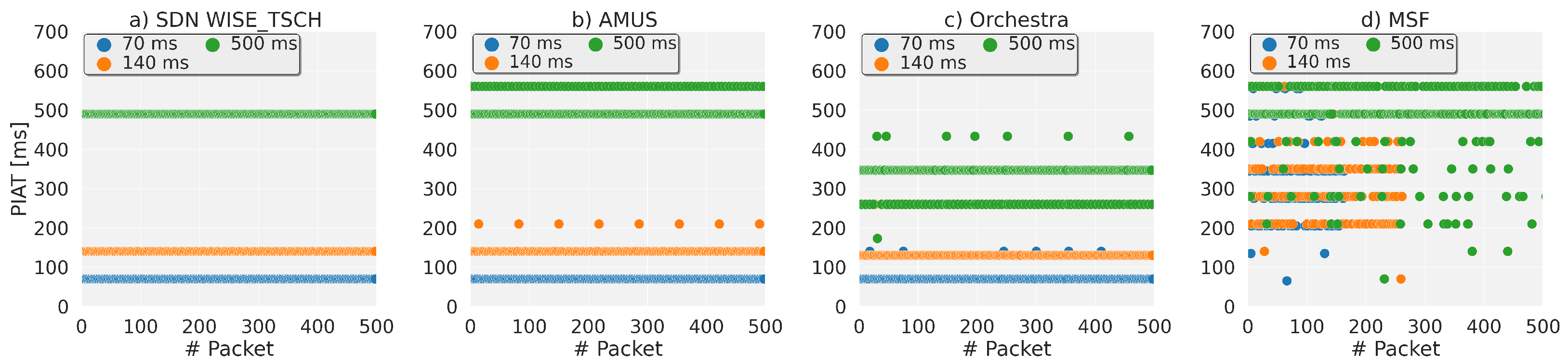
PIAT is a metric that verifies the effect of all the traffic flowing through the network on a specific data flow. The closer this value is to the Packet Period, the more deterministic the network is, since the delay added by the intermediate hops is constant. In this case, Figure 6 shows the results for different values of the Packet Period on each of the TSCH schedulers.

For Figure 6a SDN WISE-TSCH, 3 clearly differentiated lines can be observed, corresponding to each of the flows (70 ms, 140 ms and 500 ms). These are constant and coincide with the packet period because the packets are classified and sent by the specific resources assigned to them. In AMUS Figure 6b the only flow that maintains a constant delay is the 70 ms flow, beacause its frequency always has packets in queue. The other flows show variations that even exceed the established deadline because there is no synchronisation between TSCH scheduling and packet generation. For Orchestra in Figure 6c all the flows have variations, produced by the saturation of the nodes. However, the low saturation of Orchestra buffers allows it to outperform AMUS since more than 100% of the packets are below 500 ms. In Figure 6d the MSF behaviour has a high randomness for flows with higher frequency, 70 ms and 140 ms, because when using the shared slots collisions can occur at any hop. In low saturation conditions, it has more stable behaviour with 80% of the packets at around 500 ms.

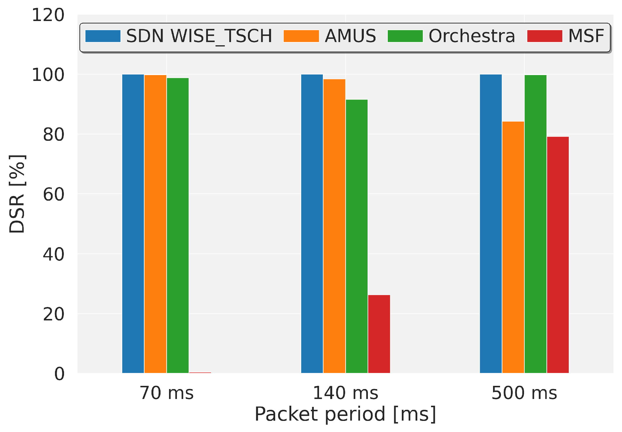
The DSR makes it possible to cumulatively observe the total number of packets that are received in a time less than or equal to the packet period. A high DSR value entails a constant and predictable flow between the source and the destination, which leads to greater determinism. In Figure 7, SDN WISE-TSCH achieves a deadline satisfaction rate of 100% in all cases due to the fact that in this scheduler the flows are differentiated and the TSCH scheduling adapted to be below the deadline. AMUS achieves 98%, 90% and 84% due to the lack of synchronisation between generation and scheduling, which can cause the transmission to be delayed with the next slotframe. When this happens the control packets can be sent by the cells assigned to the data traffic. Orchestra maintains a high DSR in all cases 95%, 90% and 95% but like AMUS, it is affected by control traffic that it cannot differentiate. However, for high packet generation periods it is not affected because the bandwidth does not depend on the scheduled traffic, it depends on the slotframe length. Therefore, in this case Orchestra has a larger amount of bandwidth available. MSF reaches 79% under favourable conditions, when network congestion is low.

3.4. Multiflow Test

Previous tests analysed the behaviour of the network independently for each traffic flow. However, due to the diversity of traffic flowing through the WSN, in industrial environments it is necessary to guarantee independently each of the flows. Therefore, in this section we will study the behaviour of the schedulers with multiple flows from the same node. For these tests, the two protocols with the highest overall performance, SDN WISE-TSCH and Orchestra, were used.

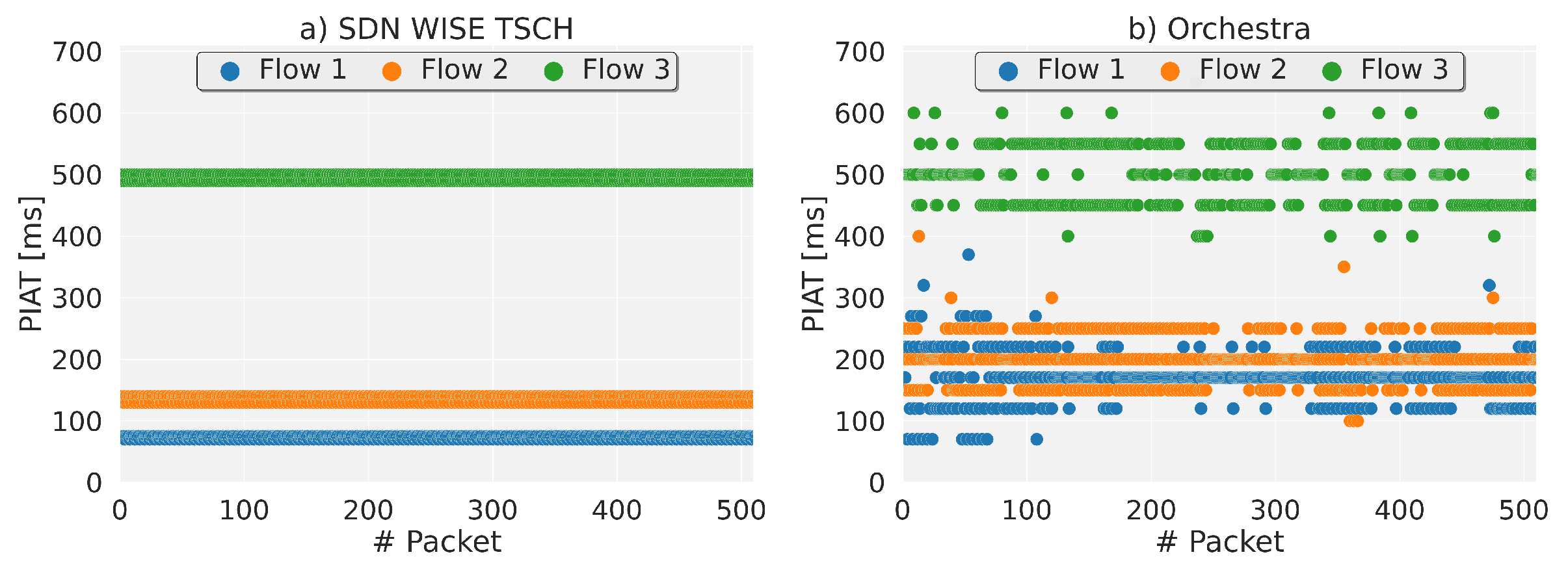
The results for the packet inter-arrival time are shown in Figure 8, with a packet period of 70 ms for flow 1, 140 ms for flow 2 and 500 ms for flow 3. The nodes transmitting these flows are 8, 9 and 10, as shown in Figure 8. Figure 8a shows how SDN WISE-TSCH performs a clear differentiation of the packets, guaranteeing regular arrival for each data flow, obtaining a DSR of 100% for both flows. in contrast with Orchestra (b) where the flows have variations that exceed the packet period. The DSR values obtained are 17%, 41% and 58%, this performance is clearly lower than that shown in Figure 6, because the network has a higher saturation and the available bandwidth is the same in both cases.

The results obtained are summarised in

Table 3. Summary of results with the different TSCH schedulers.

	SDN WISE-TSCH	AMUS	MSF	ORCHESTRA
Topology construction	SDN WISE: Beacon and Report	RPL + COAP	RPL	RPL
Latency (Delays)	Minimum	Minimum	High	Low
Reliability (PDR)	High reliability.	High	Low	High
Control Packets	Medium	High	Low	Low
Power consumption	Medium	High	Low	Low
Multiflow Performance	High	Low	Low	Medium

. SDN WISE-TSCH is the only system that can differentiate unicast flows, which allows QoS parameters to be guaranteed independently. AMUS performs similarly to WISE-TSCH SDN when there is only one unicast flow but loses determinism as the number of flows increases. This leads to increases in end-to-end delay and PIAT. Therefore, in a multiflow network its behaviour is similar to that of Orchestra, but with a much higher energy consumption. Therefore, in the testbed implementation, only the Orchestra and SDN WISE-TSCH schedulers will be used.

3.5. Testbed

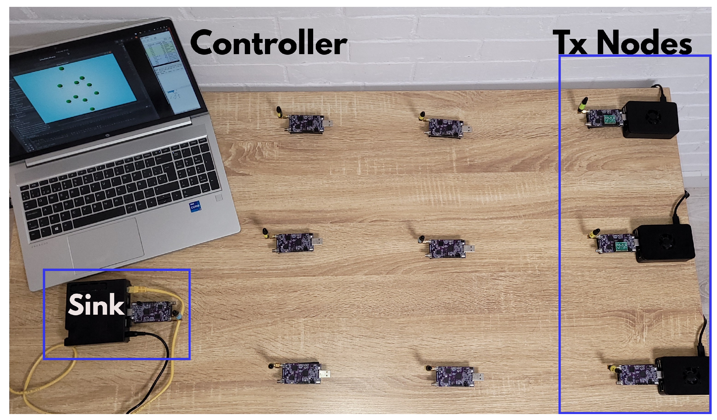
Most of the papers that evaluate scheduling algorithms only work in simulation environments and experimental evaluations are limited. In this work, in order to verify the results obtained in the simulation, the topology of Figure 3 was set up in a real environment, using 10 OpenMote B nodes with the Contiki-NG operating System. In order to obtain a multi-hop network in a reduced space, the transmission power of the nodes was set to −15 dBm, while the other parameters are the same as those used in the simulation. To capture the packets and obtain the throughput statistics, transmitting nodes 8, 9 and 10 and the destination in the Sink are connected to a Raspberry Pi. The result is the topology shown in Figure 9.

3.6. End-to-End Delay and Packet Inter-Arrival Time

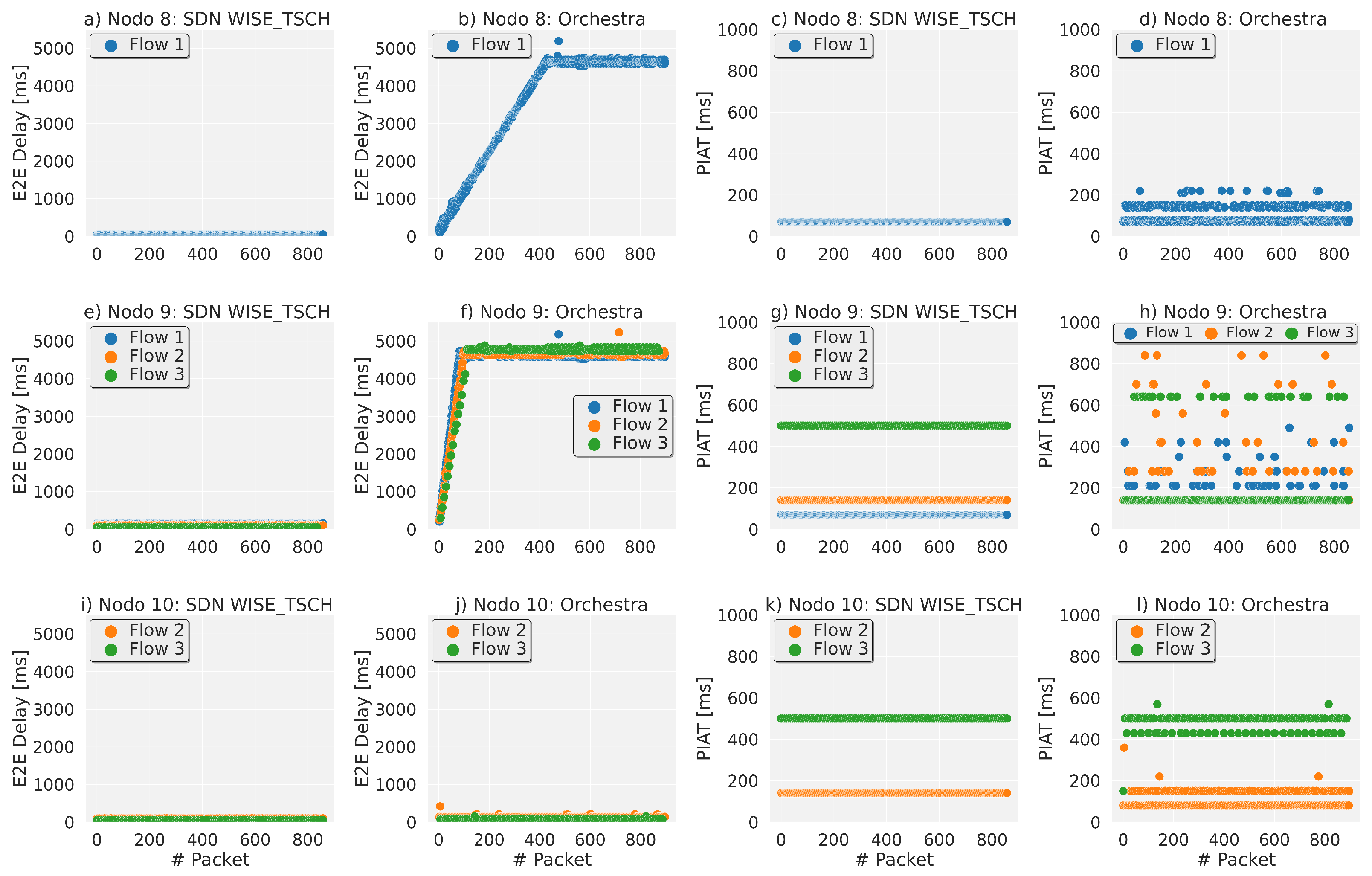
In Figure 10 the end-to-end delay and packet inter-arrival time for each of the transmitter nodes using SDN WISE-TSCH and Orchestra can be seen. The nodes have different combinations of flows assigned, as shown in Figure 3. The schedulers SDN WISE-TSCH in Figure 10a and Orchestra in Figure 10b achieve the same behaviour as in the simulation, where SDN WISE-TSCH has a minimum end-to-end delay of 50 ms for the three hops to the destination. This behaviour is typical of optimised scheduling, since it allows the source-to-destination cells between the different nodes to be linked. In Orchestra, where the cells are assigned locally so that the transmission of each hop is done in different slotframes, queuing occurs, causing the delays to increase considerably. In this case, with a slotframe of only 7 timeslots SDN WISE-TSCH achieves an end-to-end delay reduction of 75% with respect to that obtained by Orchestra. For this node, the packet inter-arrival time is constant in Figure 10c SDN WISE-TSCH, remaining at 70 ms. This, together with the low end-to-end delay, means that between source and destination there is a constant packet flow, and no delays occur at any point in the network. In contrast, Orchestra in Figure 10d shows variations of up to 380 ms. The results for node 9, which has the highest saturation case with all three flows, are shown in Figure 10e–h. SDN WISE-TSCH Figure 10e maintains the minimum end-to-end (50 ms) in the three flows due to the complete allocation of resources.

In contrast, Orchestra Figure 10f presents delays for all flows of up to 4000 ms and a high number of losses. This is due to the congestion of the queues, where Orchestra cannot configure enough bandwidth for the flows generated by the node. Because of this, the PIAT is stable in SDN WISE-TSCH Figure 10g, where it stays close to the packet generation period, while in Orchestra this lack of bandwidth is reflected with a high dispersion Figure 10h. Node 10, has the flows with the lowest bandwidth requirement, so the end-to-end delay for the two protocols in Figure 10i and Figure 10j, is very similar, with small exceptions that are due to the RPL traffic that is sent by the unicast queues. In this case the PIAT is also seen to be more bounded Figure 10k and Figure 10l, so the performance at this node is very similar for the two case studies.

3.7. Deadline Satisfaction Ratio

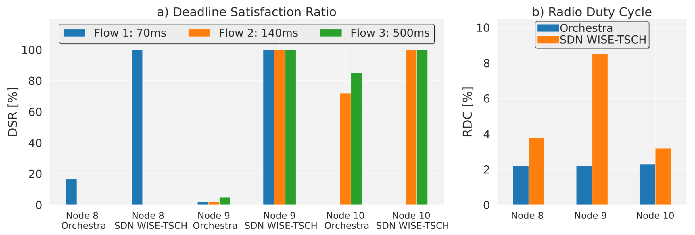
The low delays obtained by SDN WISE-TSCH and the constant PIAT values demonstrate the determinism of this proposal. This can be seen in Figure 11a, where in all nodes the deadline can be guaranteed for each flow with a rate of 100% in contrast to Orchestra which needs low saturation conditions, as was the case in node 10, to be at 85%. For node 9, which generates the most traffic, Orchestra cannot guarantee the deadlines, obtaining only 2% in the best case. Finally, for node 8, Orchestra obtains only 17%.

3.8. Radio Duty Cycle

The tests described above clearly demonstrate that SDN WISE-TSCH performs much better than Orchestra, however, it also requires higher power consumption. The RDC can be seen in Figure 11b, for each node using the two schedulers. In the first case in node 8, Orchestra has a consumption 40% lower than that obtained by SDN WISE-TSCH. For the case of higher congestion, Orchestra’s consumption is lower by 75%, but the difference in performance is also significant. Finally, in the case of node 10, where the performance is similar, the difference in performance is 28%.

4. Discussion and Conclusions

In this paper, an analysis of the quality of service obtained by different TSCH schedulers has been carried out both by simulation and testbed. The schedules obtained with SDN WISE-TSCH allow resources to be classified with greater precision, by being able to fully distinguish traffic. This results in an end-to-end delay reduction of up to 70% compared to Orchestra. In addition, a 100% deadline satisfaction rate is achieved. In multiflow conditions where the network is saturated by traffic of different characteristics, it is the only protocol that can guarantee the requirements of each type of traffic independently. Due to control traffic and increased slotframe usage, SDN results in an increase in power consumption of 28%. SDN-based schedulers have a clear QoS orientation, where traffic engineering policies with higher complexity can be applied, obtaining satisfactory results in all cases.

Schedullers such as Orchestra and MSF have the great advantage of being easy to deploy as they do not require any external intervention and all reconfiguration processes are performed locally. Their performance is good for non-critical applications. However, this performance is only achieved under low saturation conditions, when monitoring type flows are used. Moreover, in an environment with multiple information flows, they do not allow each of the flows to be guaranteed independently, resulting in increased delays and packet inter-arrival time. This moves them away from a deterministic behaviour, which is necessary in industrial environments, where each of the quality of service requirements must be guaranteed independently.

Centralised schedulers, such as AMUS, also achieve high performance in PDR and end-to-end delay due to optimised schedules. However, they have high energy consumption and present difficulties in managing control traffic. This difficulty means that they have a high variation in PIAT at the same level as distributed ones, which reduces their determinism. This is due to the lack of integration between the different layers of the protocol stack, which leads to an inflexible operation, in which it is not possible to differentiate information flows.

In summary, autonomous and distributed protocols are suitable for applications where simplicity rather than performance is required, as opposed to fully centralized protocols such as SDN, which aim for higher performance but have greater complexity. Logically, centralized protocols are an intermediate step between distributed and SDN, have the drawbacks of both and have no significant advantage.