Article

Machine Learning Model of Dimensionless Numbers to Predict Flow Patterns and Droplet Characteristics for Two-Phase Digital Flows

1
Department of Mechanical and Automation Engineering, School of Mechatronic Engineering and Automation, Shanghai University, Shanghai City 200444, China
2
Shanghai Institute of Applied Mathematics and Mechanics, School of Mechanics and Engineering Science, Shanghai University, Shanghai City 200444, China
*
Authors to whom correspondence should be addressed.
Appl. Sci. 2021, 11(9), 4251; https://doi.org/10.3390/app11094251
Submission received: 13 April 2021 / Revised: 28 April 2021 / Accepted: 5 May 2021 / Published: 7 May 2021
(This article belongs to the Section Fluid Science and Technology)

Abstract

:
In the digital microfluidic experiments, the droplet characteristics and flow patterns are generally identified and predicted by the empirical methods, which are difficult to process a large amount of data mining. In addition, due to the existence of inevitable human invention, the inconsistent judgment standards make the comparison between different experiments cumbersome and almost impossible. In this paper, we tried to use machine learning to build algorithms that could automatically identify, judge, and predict flow patterns and droplet characteristics, so that the empirical judgment was transferred to be an intelligent process. The difference on the usual machine learning algorithms, a generalized variable system was introduced to describe the different geometry configurations of the digital microfluidics. Specifically, Buckingham’s theorem had been adopted to obtain multiple groups of dimensionless numbers as the input variables of machine learning algorithms. Through the verification of the algorithms, the SVM and BPNN algorithms had classified and predicted the different flow patterns and droplet characteristics (the length and frequency) successfully. By comparing with the primitive parameters system, the dimensionless numbers system was superior in the predictive capability. The traditional dimensionless numbers selected for the machine learning algorithms should have physical meanings strongly rather than mathematical meanings. The machine learning algorithms applying the dimensionless numbers had declined the dimensionality of the system and the amount of computation and not lose the information of primitive parameters.

1. Introduction

The microfluidic technology has the advantages of generating micron or even nanometer droplets with uniform size, and it has been widely used in the fields of biology [1,2] chemistry [3], heat transfer [4], petroleum engineering [5], etc. Two-phase flow and three-phase flow [6] are common microfluids. Among them, countless papers have been focused on the flow-state modeling of microchannel two-phase flow, especially on the flow patterns and droplet characteristics that governed the droplet generation.
The prediction models [7] of flow pattern and droplet characteristics [8,9] (including the droplet length and frequency) had been established by the common method of multivariate regression analysis based on the primitive parameters in experiments. However, the physical mechanism of two-phase flow in microchannels was very complex, and the flow patterns and droplet characteristics were much sensitive to the experimental variables [10,11,12]. Thus, the prediction models were highly dependent on the experiments and could not be in extrapolation easily.
The machine learning (ML) using the algorithms to improve the accuracy of prediction model [13] had been introduced to replace the regression analysis by multivariate coupling in the microchannel two-phase flow. Timung and Mandal [14] established the ML model to predict the flow pattern of the two-phase based on the probabilistic neural network. This model input the different primitive parameters, e.g., the superficial velocity, property parameters, and geometry parameters, to predict the flow patterns in the circular microchannels (Table 1a). The comparison of prediction accuracy between the empirical model and ML model was found that the ML model had a higher accuracy for the prediction of flow pattern. Nandagopal et al. [15] studied the angle of the Y-shaped microchannel (Table 1b) and introduced the superficial velocity of two phases as the input variables. The ML model realized the prediction of flow patterns in the liquid-liquid two-phase flow. Al-Naser et al. [16] established the ML prediction model with the dimensionless Reynolds number and pressure drop multiplication factor that obtained the achievement to predict the flow patterns in a circular tube. Lin et al. [17] used the superficial velocity of two phases and inclination angles of the pipe as the input variables to predict the flow pattern of the air-water two-phase flow. Zhang et al. [18] used the ML algorithms to realize real-time flow regime identification. They found that the SVM algorithm had the best effect on the recognition of flow patterns.
Compared with lots of literature on the prediction of flow patterns using the ML models, little research had been performed to predict the droplet characteristics in the two-phase flow. At the aspect of ML, the prediction of flow patterns was a classification task, and the prediction of droplet characteristics was a regression task. Most ML models for the prediction of flow patterns used the primitive parameters directly from experiments to solve the classification task. However, for the prediction of droplet characteristics, the ML models using the primitive parameters were highly possible to fail the regression task because of the influence of dimensionality from the primitive parameters. The prediction of droplet characteristics by ML models should adopt dimensionless numbers for practice.
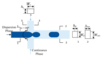
The different geometry parameters had been catalogued to be the co-flow (Table 1a), Y/T-junction (Table 1b), cross-junction (Table 1c) and tapered co-flow (Table 1d). There were multi-parameters to influence the results of flow patterns and droplet characteristics in the microchannel of two-phase digital flow. This paper cataloged all of them to be the primitive parameters, which were the geometry parameters, the process parameters, the property parameters, and the target parameters. In addition, it normalized the different geometry configurations to be the tapered co-flow model by adding two parameters of α and X (Table 1d). The implicit function equation had been established to describe the experiment system of two-phase digital flow. Then, Buckingham’s theorem [19,20,21] was applied to transform the primitive parameters to the dimensionless numbers in the implicit function. Two-group experiments with different two-phase materials had been discussed in the ML model, which used the dimensionless numbers as the input variables. The SVM algorithm was to recognize the flow patterns, and the BPNN algorithm was to predict the droplet characteristics (droplet length Ld and droplet frequency f).

2. Methods and Data

The flow chart of the ML algorithms is shown in Figure 1. Firstly, the different geometry configurations in the two-phase digital flow had been normalized with the generalized primitive parameters system. Secondly, the implicit function equation had been described by the primitive parameters and then by the dimensionless numbers on the transformation of the Buckingham theorem. Thirdly, the ML model applied the dimensionless numbers as input variables to the different algorithms. Finally, the SVM [29] algorithm achieved the classification of flow patterns, and the BPNN [30] algorithm completed the prediction of droplet characteristics in the slug and dripping patterns.
Binkhonain and Zhao [31] pointed out that the SVM algorithm was more effective and widely used among the common classification algorithms in supervised learning. The BPNN algorithm solved the suitable results on the regression tasks in different fields [32,33,34].

2.1. Generalized Variable System to Diverse Geometry Configurations

The various configurations in the microchannel had been listed with the different geometry parameters (Table 1). It was necessary to establish a generalized variable system to describe the different geometry configurations uniformly.
The rectangular and circular cross-sections were the common shapes featured by W and h, and d, respectively. They were the equivalent physical quantities obeying the following equation.
d = 2 W × h W + h
Where d is the diameter of circular, W is the width of rectangular, and h is the height of rectangular.
Compared with other publication, our team proposed a novel normalized model to the microchannel based on the convergent coaxial (or tapered co-flow) structure [27,28].
In Table 1, for the generalized variable system, it was the rectangular microchannel possessed the 8 independent geometry parameters (Wc, hc, Wd, hd, Wout, hout, X, α) more than the circular microchannel with the 5 independent geometry parameters (dc, dd, dout, X, α). The circle microchannel degenerated from the rectangular microchannel and decreased the number of geometry parameters. The rectangular microchannel often was a universal form to describe the cross-section more properly.
All the primitive parameters in experiments consisted of two parts, the independent and target variables. The independent variables included the geometry, process, and property parameters and governed the target variables. The implicit function between the independent and target variables was in Equation (2).
F g e o m e t r y ,   p r o c e s s ,   p r o p e r t y ,   t a r g e t = 0
Where geometry is geometry parameters, process is process parameters, property is property parameters, and target is droplet characteristics.
Besides the geometry parameters (Wc, hc, Wd, hd, Wout, X, α), other independent variables had different parameters, which were the process parameters of uc and ud, the property parameters of ρc, ρd, μc, μd and σ. As the target variables, it owned two parts of Ld and f. Taking all the above parameters into Equation (2), the implicit equation was reformed by 17 primitive parameters with 3 basic dimensions: M (mass), L (length), and T (time) in Equation (3).
F W c ,   h c ,   W d ,   h d ,   W o u t ,   h o u t ,   X ,   α ,   u c ,   u d ,   ρ c ,   ρ d ,   μ c ,   μ d ,   σ ,   L d ,   f = 0
Due to the influence of dimensionality, the primitive parameters cannot be weighted directly, so that they should be converted to a dimensionless form. The Buckingham theorem, widely used in other fields [20,21], was a mathematical method to transform the dimensional quantity to the dimensionless quantity. Solving the basic solutions of Equation (3) by the Buckingham theorem, 17 primitive parameters with dimensionality had been transformed into 14 dimensionless numbers (π) in Equation4.
π 1 ,   π 2 ,   ,   π 14 = 0
The above equation stated that the transformation from the primitive parameters to dimensionless numbers could decrease the dimensionality of the implicit function.
Table 2 lists the three solutions of dimensionless numbers, which are Set1, Set2, and Set3. The numbers in Set1 and Set2 were the common hydrodynamic dimensionless numbers (Oh, We, Re, St, Su, Ca [35,36,37]) with a clear physical expression. On the contrary, in Set3, the target variable (π14) was not clear on the physical expression.
The input and output variables of ML algorithms should be chosen by these dimensionless numbers. As follows, this paper discussed the ML model accuracy in the three solution sets between the two-group experiments with different materials.

2.2. Input Variables Using Dimensionless Numbers or Primitive Parameters

In an ML model, the input and output variables should be determined first. In the three dimensionless solution sets, π13 and π14 were the outputs of the variable corresponding to Ld and f, respectively. In addition, the input variables of the algorithms were determined by π112 to obey the rules. (1) They should have all specimen characteristics to represent the different experiments. (2) They should have less information redundancy to decrease the amount of computation. (3) Some of them should be ignored for the dimensionality reduction if they were invariable [38].
In order to testify the generalized variable system, this paper implemented 2 group experiments with the different two-phase flows, which were gas-liquid and liquid-liquid in the tapered co-flow microchannel. Each group experiment endured hundreds of individual experiments with different parameters. In Experiment 1 of the gas-liquid two-phase flow, the continuous phase was the solution with sodium dodecyl sulfate aqueous, and the dispersed phase was argon. In Experiment 2 of liquid-liquid two-phase flow, the continuous phase was the lubricating oil, and the dispersed phase was the deionized water. The primitive parameters of gas-liquid two-phase flow in Experiment 1 were α, ρc, μc, σ, uc, ud, and the primitive parameters of liquid-liquid two-phase flow in Experiment 2 were X, α, uc, ud.
Table 3 lists the four different sets for the ML model in 2 group experiments. There were the dimensionless numbers in Set1, Set2, and Set3 and the primitive parameters in Set4 as the input variables in the ML model. In Experiment 1, the number of input variables with the dimensionless numbers was less than 4, and it with the primitive parameters was 6. In Experiment 2, the number of input variables with dimensionless and primitive parameters was 4.
The ML model brought the different input variables with the primitive parameters and dimensionless numbers to compare the recognition accuracy of flow patterns in the two-group experiments. How to choose the appropriate dimensionless numbers to descript the generalized system was also discussed by the prediction of droplet characteristics.
The four flow patterns were identified to be slug, dripping, jetting, and others in both Experiment 1 and 2 (Figure 2). In fact, the droplet was the gas bubble in Experiment 1 and the liquid droplet in Experiment 2. Although the droplet was a dissimilar material, it had similar features in the generalized variable system.
The slug, dripping and jetting were the important flow patterns due to their formation generating the highly consistent droplets [39,40,41]. The ML model was applied to classify the four flow patterns and predict the droplet characteristics in the slug and dripping flow patterns due to enough data in experiments.

3. Results and Discussion

3.1. Recognition of Flow Patterns

The paper studied the ML model accuracy by inputting the primitive parameters and the dimensionless numbers. Before computing, all data from both Experiment 1 and 2 had been divided into the training and testing data by the ratio of 4:1, whatever they were in the solution sets with dimensionless numbers (Set1, Set2, and Set3) or primitive parameters (Set4). The training data were to establish the prediction model and the testing data were to verify the model accuracy. The accuracy of flow pattern prediction was the ratio of the number of predicted samples in the test set to the number of all samples.
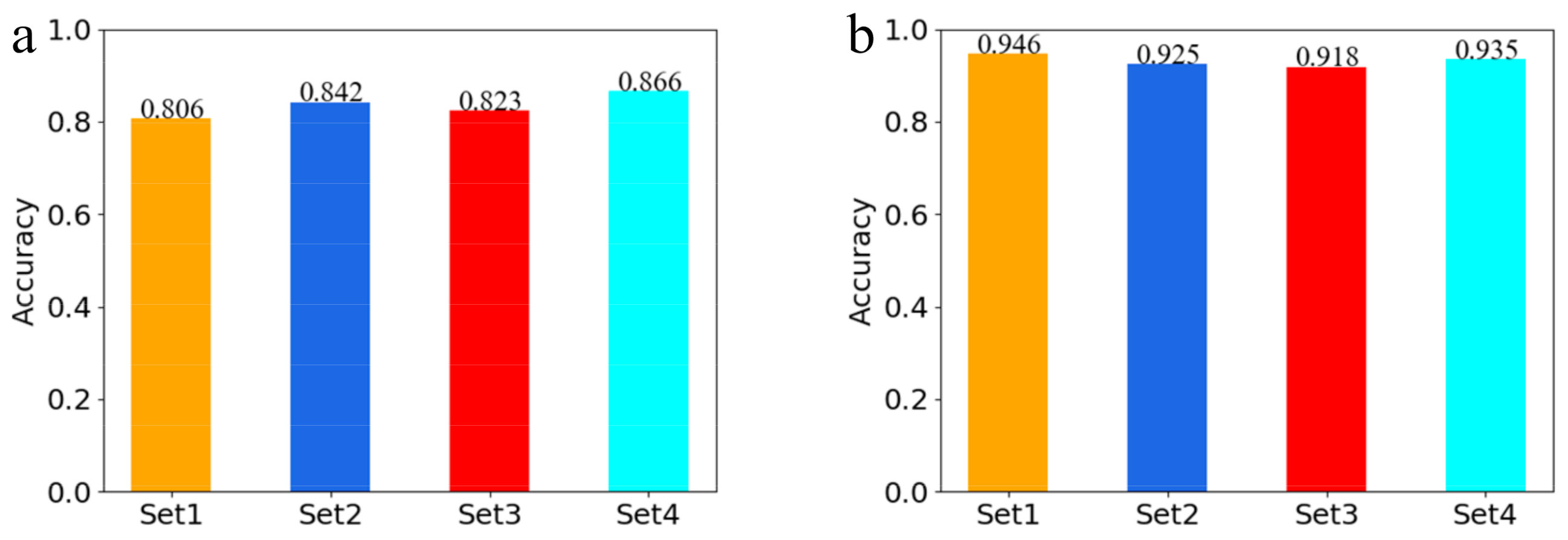
After the data partition, the SVM algorithm recognized the four flow patterns with different accuracy in both experiments (Figure 3).
It can be seen from Figure 3a that all prediction models from the solution sets with both dimensionless and primitive parameters had a similar accuracy fluctuating within the range from 80.6% (Set1) to 86.6% (Set4) in Experiment 1. On three solution sets with dimensionless numbers, the prediction accuracy in Set1, Set2, and Set3 possessed 4, 3, and 4 dimensionless numbers as the input variables in Figure 3, respectively. Set4 with the primitive parameters had six input variables higher than those in Set1, Set2, and Set3.
It was interesting that all the prediction accuracies in the four solution sets were very close. This indicated that, for the recognition of flow patterns, the SVM algorithm inputting the dimensionless numbers minimized the specimen information loss, reduced the amount of computation, and maintained the model accuracy simultaneously.
Figure 3b gives similar results in Experiment 2. The recognition accuracy is nearly consistent, about 93% in all solution sets. All dimensions of input variables are the same (4 dimensions) in both dimensionless and primitive parameters. Compared with Experiment 1, the recognition accuracy of flow patterns in Experiment 2 is higher, about 10%.
Figure 3 also proves that the recognition of flow patterns with dimensionless numbers has not decreased the model accuracy and not lost information compared with primitive parameters.
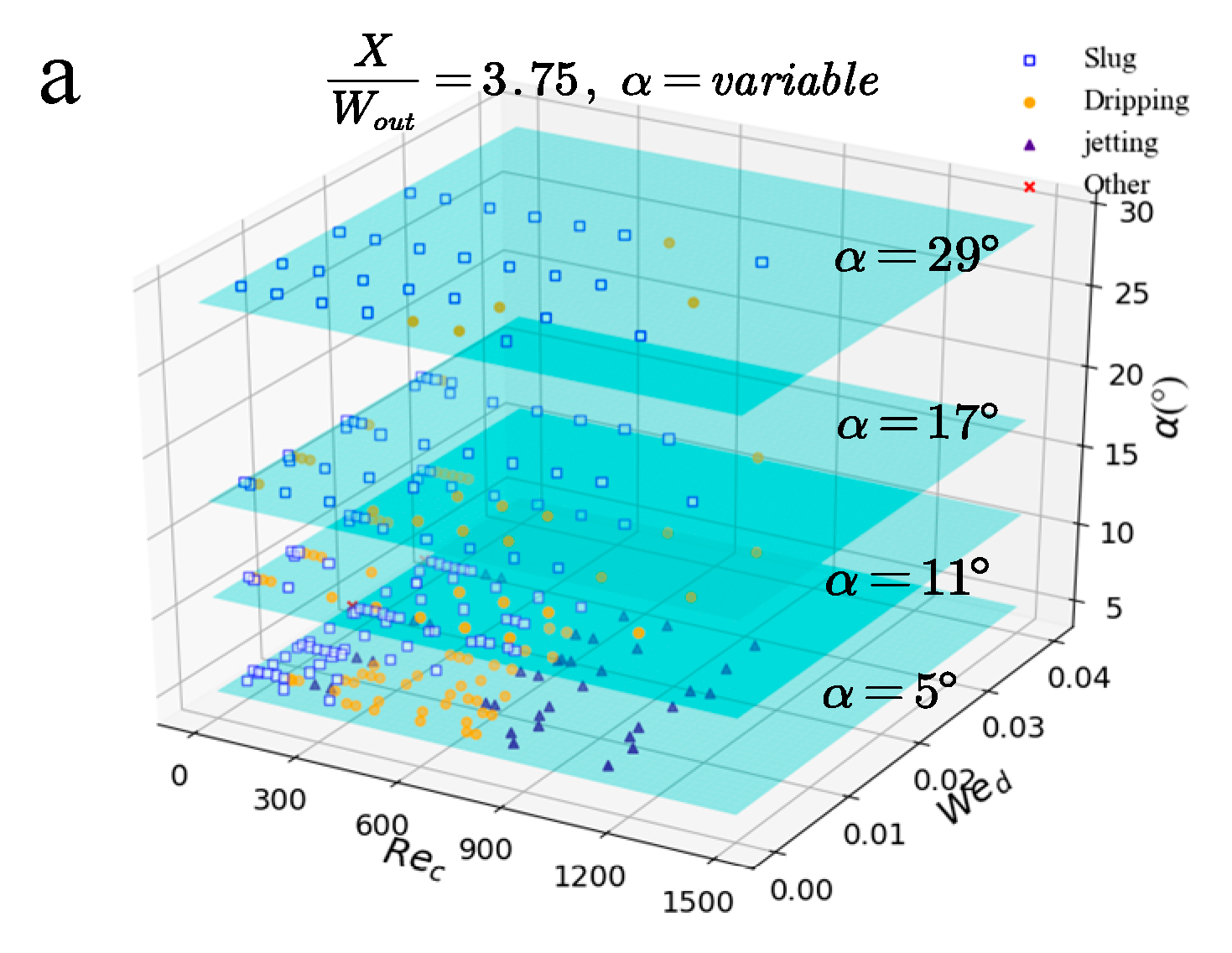
Figure 4 reveals the recognition accuracy difference between Experiment 1 and Experiment 2, taking Set2, for example. Set2 has 3 dimensionless numbers of π7, π10, and π12 (Table 3) governed by three parameters of α, Rec-, and Wed (Table 2) in Experiment 1. Setting α, Rec, and Wed as the coordinate axis, Figure 4a plots the distribution map of four flow patterns in Experiment 1. It is true that the boundaries among the different flow patterns are crossed and not clear with α changing.
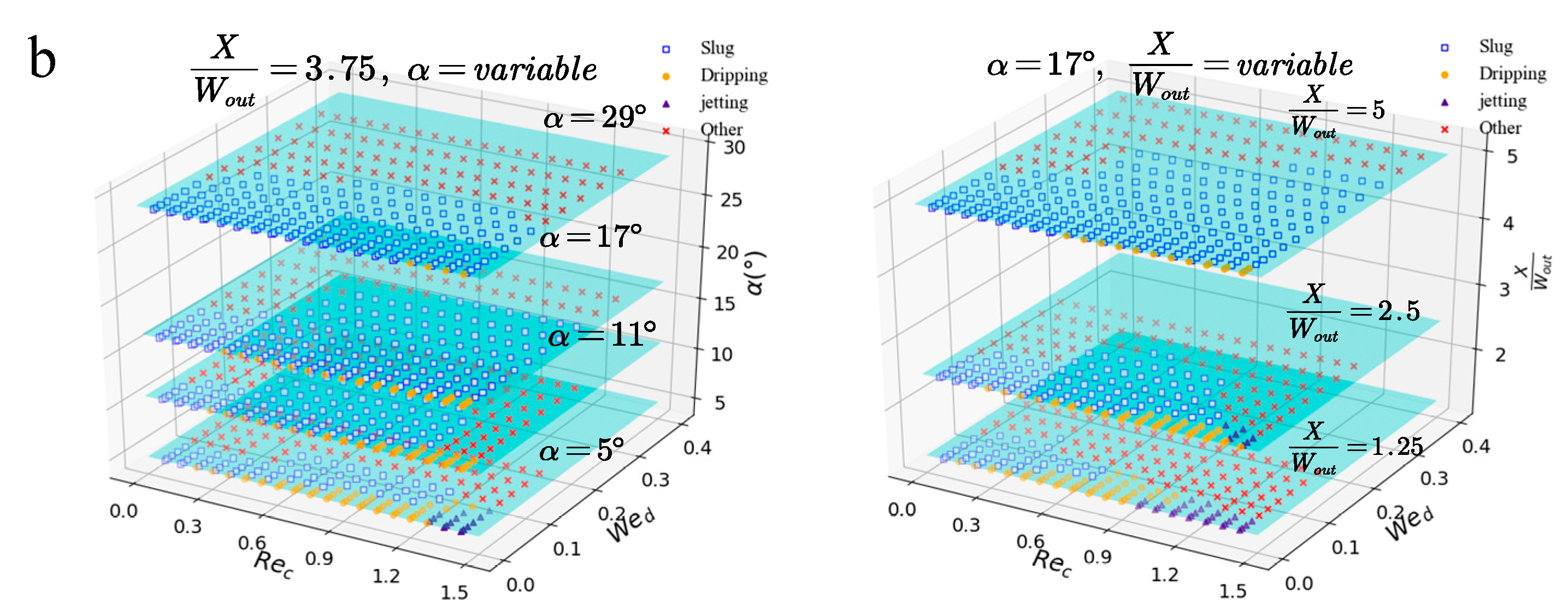
In Experiment 2, the dimensionless numbers of π6710, and π12 (Table 3) in Set2 are controlled by four parameters of X / W o u t , α, Rec, and Wed (Table 2). Setting α, Rec and Wed as the coordinate axis and X / W o u t , Rec, and Wed as the coordinate axis, respectively, the distribution maps of four flow patterns are drawn in Figure 4b. At each layer with a different α or X / W o u t value, the boundaries among the different flow patterns are very clear without any crossing.
Back to the classification task, the distinguished boundary between different data often benefits to realize the classification solution easily. Herein, the data distribution separated by the boundaries was much clear to improve the recognition accuracy significantly in Experiment 2.
Figure 4 illustrates that the difference in prediction accuracy between Experiments 1 and 2 can be attributed to the clearance of data distribution.

3.2. Prediction of Droplet Characteristics

The primitive parameters could not be used as the input variables to predict the droplet characteristics since they would make the prediction model lose the physical meaning. Therefore, this paper only discussed the different solution sets with dimensionless numbers to predict the droplet characteristics.
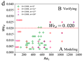
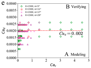
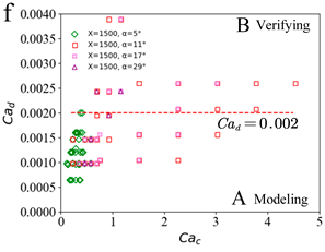
The data sets of Experiments 1 and 2 had been divided into two parts, Region A and Region B, with the ratio of about 4:1, in which the data in Region A and Region B were used to establish and verify the prediction model. In Region A, the data were further divided into the training data and testing data with the ratio of 4:1.
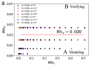
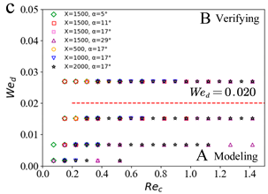
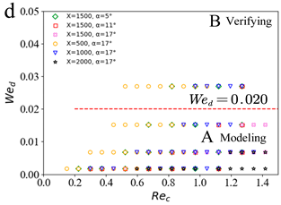
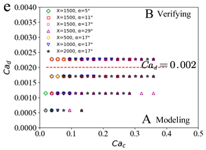
The data partition of slug and dripping patterns in Set1 was separated by the line with Wed=0.02 in Experiment 1 (Table 4a,b). The data in Region B was above this line, inversely the data in Region A was below it. Similarly, the data partition of slug and dripping patterns in Set2 and Set3 were separated by the line with Wed = 0.02 and Cad = 0.002, respectively (Table 4c–f).
Table 5 is the data partition of slug and dripping patterns in three sets in Experiment 2. The partition line adopted the same parameters following it in Experiment 1.
The BPNN algorithm was guided to predict the droplet characteristics, which were π13 and π14. Before the data inputting, the normalized x’ ∈ (0,1) was identified to increase the convergence of the algorithm (Equation (5)).
x = x x m i n x m a x x m i n
Where x is the number value, x’ is the normalized number value, and xmax and xmin are maximum and minimum values of x, respectively.
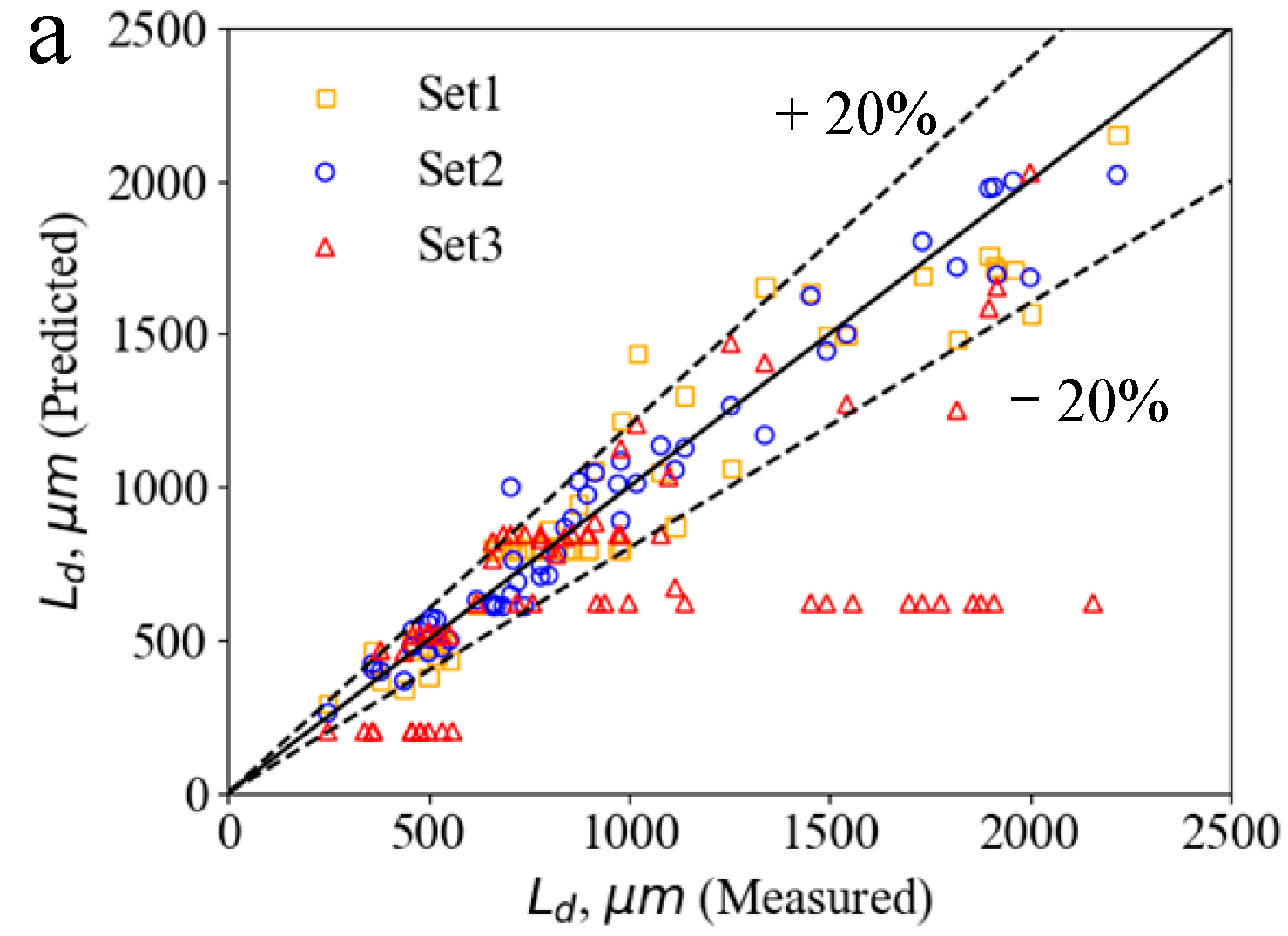
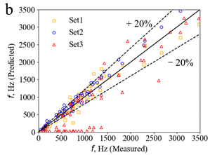
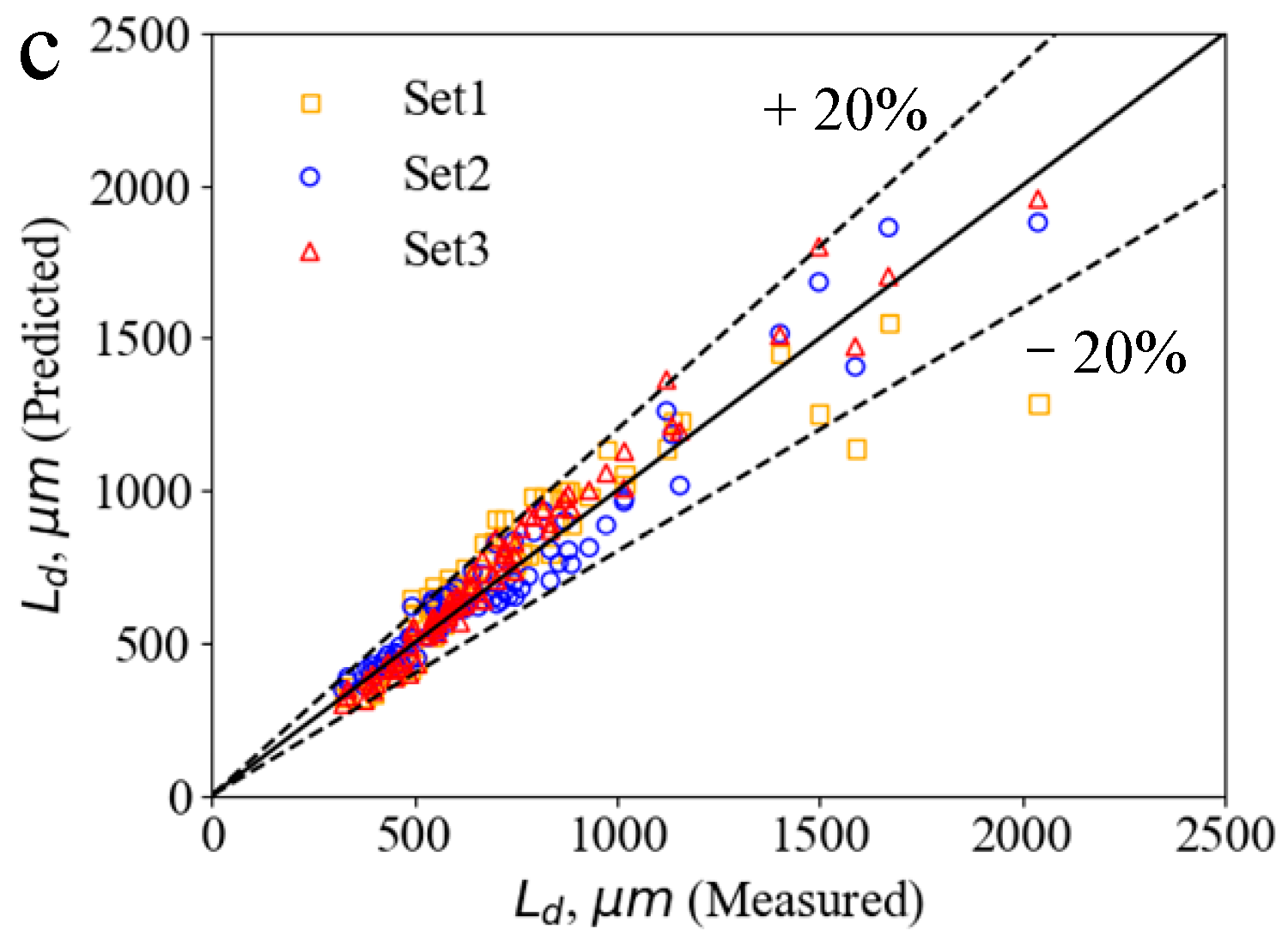
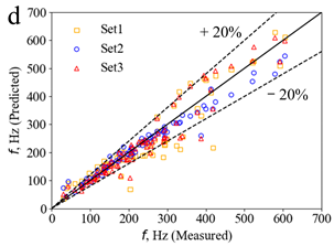
After normalization, the data in Region A had been input to the BPNN algorithm establishing the prediction model of droplet characteristics in different sets. Then the data in Region B were input to the prediction model predicting π13 and π14 and getting the result the parameters (Ld and f) by inversed operation. Table 6 shows the model errors of slug and dripping patterns predicted by three sets in Experiment 1 and Experiment 2. The errors were obtained by comparing the predicted value with the measured value in all samples from Region B.
According to Experiment 1, the model errors of droplet characteristics in slug and dripping patterns are shown in Table 6a,b. Compared with the measured values, the prediction model of droplet length Ld and droplet frequency f in slug pattern occupied the error range within ± 20% both in Set1 and Set2, and more than ± 20% in Set3 (Table 6a). The same phenomenon was found in the dripping pattern (Table 6b).
The model errors of droplet characteristics, Ld and f, in slug and dripping patterns in Experiment 2 were shown in Table 6c,d. It was clear that, compared with the measured values, the model errors of length Ld and frequency f in slug droplet were in the range of ± 20% regardless of Set1, Set2, and Set3 (Table 6c). Similarly, the prediction model occupied the error in ± 20% comparing with the measured values in dripping pattern in all three sets (Table 6d).
It was true that the model error of Set3 was worse than it of Set1 and Set2 in Experiment 1; however, that of Set1, Set2, and Set3 in Experiment 2 was similar. The accuracy difference of the prediction model among the three sets was mainly expressed by the relationship between dimensionless numbers and their physical meanings.
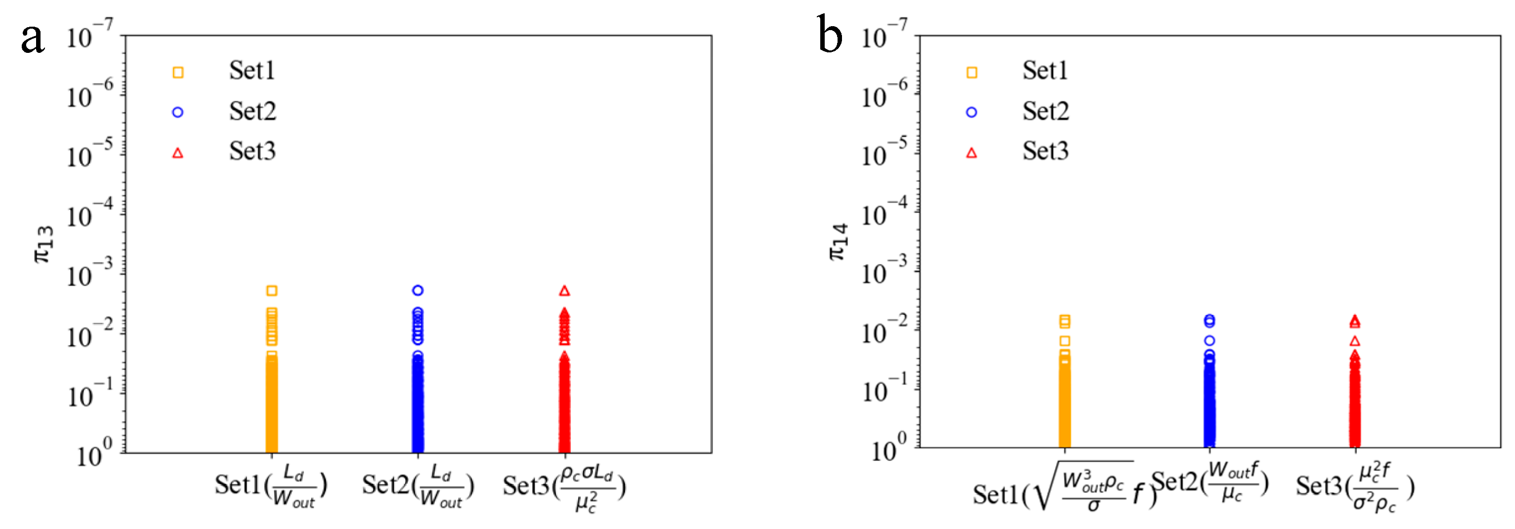
In all three sets, the predicted parameters of Ld and f were mapped by the dimensionless numbers of π13 and π14. It was obvious that the accuracy difference with slug and dripping patterns in different experiments had been strongly related to the values of π13 and π14 (Figure 5 and Figure 6).
In the slug and dripping patterns of Experiment 1, the order of magnitude of π13 value changed from 10−3 to 100 in Set1 and Set2 and from 10−4 to 100 in Set3. There was one order of magnitude gap of π13 value between Set1, Set2, and Set3 (Figure 5a). Similarly, the order of magnitude of π14 value changed from 10−3 to 100 in Set1 and Set2 and from 10−7 to 100 in Set3. There was a four order of magnitude gap of π14 value between Set1, Set2, and Set3 (Figure 5b). It demonstrated that the dimensionless numbers of π13 and π14 in Set3 had a widely separate distribution than those in Set1 and Set2, which led to the accuracy decline for the prediction model.
Figure 6 shows the data distribution of π13 and π14 in Experiment 2. All the values of π13 and π14 in three sets had the order of magnitude range from 10−3 to 100 without the distinguish gap among them. As a result, the prediction accuracy of droplet characteristics with three sets in Experiment 2 was a similar value, and this was higher than it in Experiment 1. This also proved that the smaller range of dimensionless numbers distribution could improve the model accuracy significantly.
It should be emphasized that the solutions were not only one set but also infinite sets by using Buckingham’s theorem transforming the primitive variable equation to a dimensionless variable equation. Although all solution sets were mathematically equivalent, the different solution sets described the same physical system in different ways. In the three sets, π14 had three different forms (Set1: W 3 out ρ c σ f , Set2: W o u t f μ c S t , Set3:   μ c 3 f ρ c ) to correspond to the same physical system. The expression of π14 in Set1 and Set2 was traditional hydromechanics dimensionless numbers stated by literature in Table 2, and it in Set3 was not common to describe the physical system clearly. It was known that Set3 was a random solution from the infinite solutions. To achieve higher prediction accuracy, the solution set selected from the dimensionless implicit function should be in the physical meaning strongly instead of considering the mathematical meaning only. The range of data distribution could be used as the criterion to judge whether the solution set had the stronger physical meaning in the ML model with dimensionless numbers.

4. Conclusions

This paper introduced a generalized variable system to describe the different geometry configurations of the microchannel. Buckingham’s theorem transformed the primitive parameters into dimensionless numbers using the implicit function equation. Taking the dimensionless numbers to input the machine learning model, the SVM algorithm had recognized the flow patterns, and the BPNN algorithm predicted the droplet characteristics.
The model accuracy of flow patterns with dimensionless or primitive parameters was almost the same by the SVM algorithm in the same group of experiments. There was an accuracy variation between the two-group experiments, and its main reason was that the boundaries between the adjacent flow patterns were not clear and crossed each other. According to the primitive parameters, the prediction model applying the dimensionless numbers had reduced the dimensionality of input variables, saved the computing time, and maintained the model accuracy.
The infinite solutions of dimensionless numbers were equivalent in the mathematical meaning. However, the prediction accuracy of droplet characteristics was not the same in the different solution sets. It was explained directly that the discrete data of dimensionless numbers (π13 and π14) had significant and negative effects on the model accuracy based on the two-group experiments. Furthermore, all solution sets with the equivalent mathematical meaning were not in the same physical meaning. In order to achieve higher prediction accuracy, the solution set selection should be in physical meaning strongly, and the range of data distribution should be used narrowly.
We had been established the normalized model for the two-phase flow in this paper. However, how to use the model to the multiphase flow (e.g., three-phase flow) correctly is still necessary to be researched further by improving the model. On the other hand, the experiments in this paper only supported the normalized geometry configurations of the model. As the experiment material changes, the effects of physical parameters should be considered carefully in the implicit function.

Author Contributions

Conceptualization, writing—review and editing and supervision, J.Z. (Jinsong Zhang) and Z.W.; software, formal analysis, investigation and writing—original draft preparation, S.Z.; project administration, J.Z. (Jianhua Zhang); All authors have read and agreed to the published version of the manuscript.

Funding

This research was funded by National Key Research and Development Program of China, project name: 8.5 Generation Printing OLED Display Industrial Demonstration Project, grant number: 2017YFB0404503.

Institutional Review Board Statement

The study did not involve humans or animals.

Informed Consent Statement

The study did not involve humans or animals.

Data Availability Statement

The study did not report any data.

Conflicts of Interest

The authors declare no conflict of interest.

Nomenclature

Wcthe width of the continuous phase tube (μm)uthe superficial velocity (m/s)
hcthe height of the continuous phase tube (μm)Ldthe length of the droplet (μm)
dcthe diameter of the continuous phase tube (μm)fthe frequency of the droplet (Hz)
Wdthe width of the dispersed phase tube (μm)Greek characters
hdthe height of the dispersed phase tube (μm)σthe surface tension (N/m)
ddthe diameter of the dispersed phase tube (μm)ρthe density (kg/m3)
Woutthe width of the outlet tube (μm)μthe dynamic viscosity (Pa•s)
houtthe height of the outlet tube (μm)Subscripts
doutthe diameter of the outlet tube (μm)cthe continuous phase
Xthe displacement of the injection nozzle (μm)dthe dispersed phase
αthe tapered angle (rad)outthe outlet tube

References

  1. Sheidaei, Z.; Akbarzadeh, P.; Kashaninejad, N. Advances in numerical approaches for microfluidic cell analysis platforms. J. Sci. Adv. Mater. Dev. 2020, 5, 295–307. [Google Scholar] [CrossRef]
  2. Hongzhou, C.; Shuping, G.; Wenju, W.; Li, L.; Lulu, W.; Linjun, D.; Jingmin, L.; Xiaoli, R.; Li, B. Lab-on-a-chip technologies for genodermatoses: Recent progress and future perspectives. J. Dermatol. Sci. 2017, 85, 71–76. [Google Scholar] [CrossRef]
  3. Batool, S.; Nawaz, M. Investigation of thermal enhancement in non-Newtonian fluid with hybrid micro-structures in an enclosure. Int. Commun. Heat Mass Transf. 2020, 117. [Google Scholar] [CrossRef]
  4. Keniar, K.; El Fil, B.; Garimella, S. A critical review of analytical and numerical models of condensation in microchannels. Int. J. Refrig. 2020, 120, 314–330. [Google Scholar] [CrossRef]
  5. Roshani, M.; Sattari, M.A.; Muhammad Ali, P.J.; Roshani, G.H.; Nazemi, B.; Corniani, E.; Nazemi, E. Application of GMDH neural network technique to improve measuring precision of a simplified photon attenuation based two-phase flowmeter. Flow Measur. Instrum. 2020, 75, 101804. [Google Scholar] [CrossRef]
  6. Roshani, M.; Phan, G.; Hossein Roshani, G.; Hanus, R.; Nazemi, B.; Corniani, E.; Nazemi, E. Combination of X-ray tube and GMDH neural network as a nondestructive and potential technique for measuring characteristics of gas-oil–water three phase flows. Measurement 2021, 168, 108427. [Google Scholar] [CrossRef]
  7. Wu, Z.; Sundén, B. Liquid-liquid two-phase flow patterns in ultra-shallow straight and serpentine microchannels. Heat Mass Transf. 2018, 55, 1095–1108. [Google Scholar] [CrossRef] [Green Version]
  8. Erb, R.M.; Obrist, D.; Chen, P.W.; Studer, J.; Studart, A.R. Predicting sizes of droplets made by microfluidic flow-induced dripping. Soft Matter 2011, 7, 8757–8761. [Google Scholar] [CrossRef]
  9. Gu, Y.; Kojima, H.; Miki, N. Theoretical analysis of 3D emulsion droplet generation by a device using coaxial glass tubes. Sensors Actuators A Phys. 2011, 169, 326–332. [Google Scholar] [CrossRef]
  10. Lian, J.; Luo, X.; Huang, X.; Wang, Y.; Xu, Z.; Ruan, X. Investigation of microfluidic co-flow effects on step emulsification: Interfacial tension and flow velocities. Colloids Surfaces A Physicochem. Eng. Aspects 2019, 568, 381–390. [Google Scholar] [CrossRef]
  11. Du, J.; Ibaseta, N.; Guichardon, P. Generation of an O/W emulsion in a flow-focusing microchip: Importance of wetting conditions and of dynamic interfacial tension. Chem. Eng. Res. Des. 2020, 159, 615–627. [Google Scholar] [CrossRef]
  12. Rajiv, K.H.; Singh Sokhal, G. Effect of geometries and nanofluids on heat transfer and pressure drop in microchannels: A review. Mater. Today Proc. 2020, 28, 1841–1846. [Google Scholar] [CrossRef]
  13. Roshani, M.; Phan, G.T.T.; Jammal Muhammad Ali, P.; Hossein Roshani, G.; Hanus, R.; Duong, T.; Corniani, E.; Nazemi, E.; Mostafa Kalmoun, E. Evaluation of flow pattern recognition and void fraction measurement in two phase flow independent of oil pipeline’s scale layer thickness. Alex. Eng. J. 2021, 60, 1955–1966. [Google Scholar] [CrossRef]
  14. Timung, S.; Mandal, T.K. Prediction of flow pattern of gas–liquid flow through circular microchannel using probabilistic neural network. Appl. Soft Comput. 2013, 13, 1674–1685. [Google Scholar] [CrossRef]
  15. Nandagopal, M.S.G.; Abraham, E.; Selvaraju, N. Advanced neural network prediction and system identification of liquid-liquid flow patterns in circular microchannels with varying angle of confluence. Chem. Eng. J. 2017, 309, 850–865. [Google Scholar] [CrossRef]
  16. Al-Naser, M.; Elshafei, M.; Al-Sarkhi, A. Artificial neural network application for multiphase flow patterns detection: A new approach. J. Petrol. Sci. Eng. 2016, 145, 548–564. [Google Scholar] [CrossRef]
  17. Lin, Z.; Liu, X.; Lao, L.; Liu, H. Prediction of two-phase flow patterns in upward inclined pipes via deep learning. Energy 2020, 210, 118541. [Google Scholar] [CrossRef]
  18. Zhang, Y.; Azman, A.N.; Xu, K.-W.; Kang, C.; Kim, H.-B. Two-phase flow regime identification based on the liquid-phase velocity information and machine learning. Exp. Fluids 2020, 61, 62–72. [Google Scholar] [CrossRef]
  19. Buckingham, E. On physically similar systems; illustrations of the use of dimensional equations. Phys. Rev. 1914, 4, 345–376. [Google Scholar] [CrossRef]
  20. Kumbhar, S.G.; Sudhagar, P.E.; Desavale, R.G. Theoretical and experimental studies to predict vibration responses of defects in spherical roller bearings using dimension theory. Measurement 2020, 161, 107846. [Google Scholar] [CrossRef]
  21. Tang, R.C.O.; Jang, J.-H.; Lan, T.-H.; Wu, J.-C.; Yan, W.-M.; Sangeetha, T.; Wang, C.-T.; Ong, H.C.; Ong, Z.C. Review on design factors of microbial fuel cells using Buckingham’s Pi Theorem. Renew. Sustain. Energy Rev. 2020, 130. [Google Scholar] [CrossRef]
  22. Cramer, C.; Fischer, P.; Windhab, E.J. Drop formation in a co-flowing ambient fluid. Chem. Eng. Sci. 2004, 59, 3045–3058. [Google Scholar] [CrossRef]
  23. Hua, J.; Zhang, B.; Lou, J. Numerical simulation of microdroplet formation in coflowing immiscible liquids. AIChE J. 2007, 53, 2534–2548. [Google Scholar] [CrossRef]
  24. Chaves, I.L.; Duarte, L.C.; Coltro, W.K.T.; Santos, D.A. Droplet length and generation rate investigation inside microfluidic devices by means of CFD simulations and experiments. Chem. Eng. Res. Des. 2020, 161, 260–270. [Google Scholar] [CrossRef]
  25. Huang, D.; Wang, K.; Wang, Y.; Sun, H.; Liang, X.; Meng, T. Precise control for the size of droplet in T-junction microfluidic based on iterative learning method. J. Frankl. Inst. 2020, 357, 5302–5316. [Google Scholar] [CrossRef]
  26. Bai, L.; Zhao, S.; Fu, Y.; Cheng, Y. Experimental study of mass transfer in water/ionic liquid microdroplet systems using micro-LIF technique. Chem. Eng. J. 2016, 298, 281–290. [Google Scholar] [CrossRef]
  27. Wang, Z.L. Speed up bubbling in a tapered co-flow geometry. Chem. Eng. J. 2015, 263, 346–355. [Google Scholar] [CrossRef]
  28. Zhang, J.; Wang, C.; Liu, X.; Yi, C.; Wang, Z.L. Experimental studies of microchannel tapering on droplet forming acceleration in liquid paraffin/ethanol coaxial flows. Materials 2020, 13, 944. [Google Scholar] [CrossRef] [Green Version]
  29. Cortes, C.; Vapnik, V. Support-vector networks. Mach. Learn. 1995, 20, 273–297. [Google Scholar] [CrossRef]
  30. Rumelhart, D.E.; Hinton, G.E.; Williams, R.J. Learning representations by back propagating errors. Nature 1986, 323, 533–536. [Google Scholar] [CrossRef]
  31. Binkhonain, M.; Zhao, L. A review of machine learning algorithms for identification and classification of non-functional requirements. Expert Syst. Appl. X 2019, 1, 100001. [Google Scholar]
  32. Vijayanand, M.; Varahamoorthi, R.; Kumaradhas, P.; Sivamani, S.; Kulkarni, M.V. Regression-BPNN modelling of surfactant concentration effects in electroless Ni B coating and optimization using genetic algorithm. Surface Coat. Technol. 2021, 409, 126878. [Google Scholar] [CrossRef]
  33. Ma, Z.; Zhang, W.; Luo, Z.; Sun, X.; Li, Z.; Lin, L. Ultrasonic characterization of thermal barrier coatings porosity through BP neural network optimizing Gaussian process regression algorithm. Ultrasonics 2020, 100, 105981. [Google Scholar] [CrossRef]
  34. Ni, Y.Q.; Li, M. Wind pressure data reconstruction using neural network techniques: A comparison between BPNN and GRNN. Measurement 2016, 88, 468–476. [Google Scholar] [CrossRef]
  35. Akbar, M.K.; Plummer, D.A.; Ghiaasiaan, S.M. On gas–liquid two-phase flow regimes in microchannels. Int. J. Multiphase Flow 2003, 29, 855–865. [Google Scholar] [CrossRef]
  36. Laborie, S.; Cabassud, C.; Durandbourlier, L.; Laine, J.M. Characterisation of gas-liquid two-phase flow inside capillaries. Chem. Eng. Sci. 1999, 54, 5723–5735. [Google Scholar] [CrossRef]
  37. Hernández-Cid, D.; Pérez-González, V.H.; Gallo-Villanueva, R.C.; González-Valdez, J.; Mata-Gómez, M.A. Modeling droplet formation in microfluidic flow-focusing devices using the two-phases level set method. Mater. Today Proc. 2020. [Google Scholar] [CrossRef]
  38. Chaichana, C.; Thiangchanta, S. The heat load modelling for an air-conditioned room using Buckingham-Pi theorem. Energy Rep. 2020, 6, 656–661. [Google Scholar] [CrossRef]
  39. Zhao, Y.; Chen, G.; Yuan, Q. Liquid-liquid two-phase flow patterns in a rectangular microchannel. AIChE J. 2006, 52, 4052–4060. [Google Scholar] [CrossRef]
  40. Liu, X.; Wu, L.; Zhao, Y.; Chen, Y. Study of compound drop formation in axisymmetric microfluidic devices with different geometries. Colloids Surfaces A Physicochem. Eng. Aspects 2017, 533, 87–98. [Google Scholar] [CrossRef]
  41. Liu, C.; Zhang, Q.; Zhu, C.; Fu, T.; Ma, Y.; Li, H.Z. Formation of droplet and “string of sausages” for water-ionic liquid ([BMIM][PF6]) two-phase flow in a flow-focusing device. Chem. Eng. Process. Process Intensif. 2018, 125, 8–17. [Google Scholar] [CrossRef]
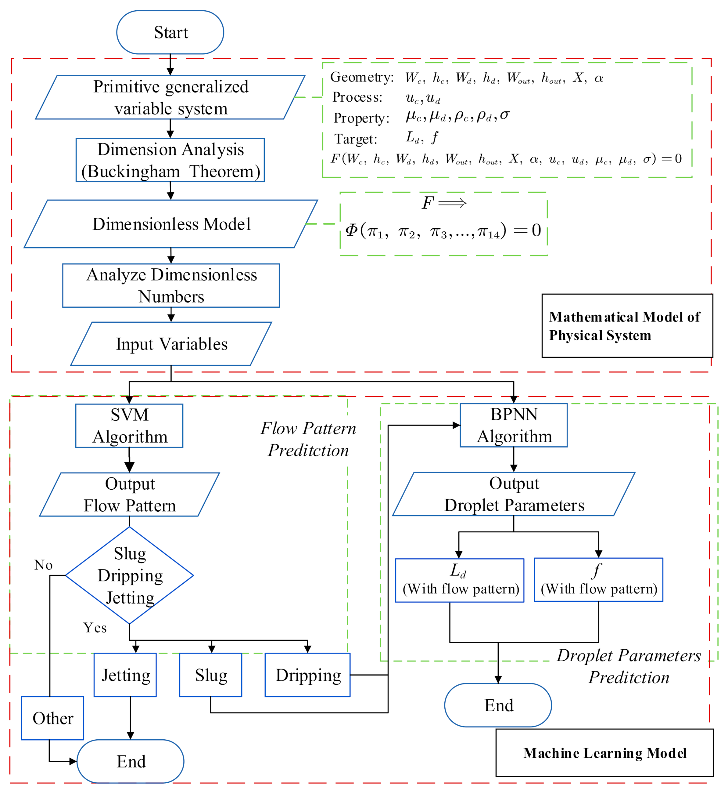
Figure 1. Flow chart of machine learning algorithms.
Applsci 11 04251 g001
Figure 2. Four flow patterns in both Experiment 1 (gas-liquid) and Experiment 2 (liquid-liquid). (a) Slug, (b) dripping, (c) jetting, (d) other.
Applsci 11 04251 g002
Figure 3. The recognition accuracy of flow patterns by SVM algorithm, (a) Experiment 1: gas-liquid two-phase flow, (b) Experiment 2: liquid-liquid two-phase flow.
Applsci 11 04251 g003
Figure 4. The flow patterns diagram of 2 group experiments: (a) Experiment 1, (b) Experiment 2.
Applsci 11 04251 g004aApplsci 11 04251 g004b
Figure 5. Value ranges of π13 and π14 for three sets with slug and dripping patterns in Experiment 1: (a) π13, (b) π14.
Applsci 11 04251 g005
Figure 6. Value ranges of π13 and π14 for three sets with slug and dripping patterns in Experiment 2: (a) π13, (b) π14.
Applsci 11 04251 g006
Table 1. Normalized model for different geometry configurations in the microchannel.
CitationTypeGeometry StructureInlet ParametersOutlet ParametersCross-SectionNormalized Parameters
aCramer et al. [22]
Hua et al. [23]
co-flow Applsci 11 04251 i001dc, dddoutcircular3
bChaves et al. [24]
Huang et al. [25]
Y/T-junction Applsci 11 04251 i002Wc, hc, Wd, hd, αWout, houtrectangle7
cBai et al. [26]cross-junction Applsci 11 04251 i003Wd, hd, Wc, hc, α=180°Wout, houtrectangle7
dOur team [27,28]tapered co-flow Applsci 11 04251 i004X, α, dc, dddoutcircular5
Applsci 11 04251 i005Wc, hc, Wd, hd, X, αWout, houtrectangle8
Table 2. Three typical solutions of dimensionless numbers (π).
πSet1Set2Set3
Independent Variablesπ1 h o u t W o u t h o u t W o u t μ d μ c
π2 W c W o u t W c W o u t ρ d ρ c
π3 h c W o u t h c W o u t ρ c σ X μ c 2 S u c
π4 W d W o u t W d W o u t μ c u c σ C a c
π5 d d W o u t d d W o u t μ d u d σ C a d
π6 X W o u t X W o u t α
π7 α α ρ c σ W o u t μ c 2
π8 ρ d ρ c μ d μ c ρ c σ h o u t μ c 2
π9 μ c W o u t ρ c σ O h c ρ d ρ c ρ c σ W c μ c 2
π10 μ d W o u t ρ d σ O h d W o u t ρ c u c μ c R e c ρ c σ h c μ c 2
π11 W o u t ρ c u c 2 σ W e c W o u t ρ d u d μ d R e d ρ c σ W d μ c 2
π12 W o u t ρ d u d 2 σ W e d W o u t ρ d u d 2 σ W e d ρ c σ d d μ c 2
Target Variablesπ13 L d W o u t L d W o u t ρ c σ L d μ c 2
π14 W 3 ρ c σ f W o u t f μ c S t μ c 3 f ρ c
Table 3. Input variables using dimensionless numbers and primitive parameters in the ML model.
Dimensionless NumbersPrimitive Parameters
Equation ϕ π 1 , π 2 , π 3 , , π 14 = 0 F ( W c , h c , W d , h d , W o u t , h o u t , X ,   α , u c , u d , ρ c , ρ d , μ c , μ d , σ , L d , f ) = 0
SetSet1Set2Set3Set4
Input variables
(Experiment 1)
π7, π9, π11, π12
(4 Dimensions)
π7, π10, π12
(3 Dimensions)
π3, π4, π5, π6
(4 Dimensions)
α, uc, ud, ρc, μc, σ
(6 Dimensions)
Input variables
(Experiment 2)
π6, π7, π11, π12
(4 Dimensions)
π6, π7, π10, π12
(4 Dimensions)
π3, π4, π5, π6
(4 Dimensions)
X, α, uc, ud
(4 Dimensions)
Table 4. Data partition of three sets with dimensionless numbers in Experiment 1: (a) slug in Set1, (b) dripping in Set1, (c) slug in Set2, (d) dripping in Set2, (e) slug in Set3, and (f) dripping in Set3.
Slug PatternDripping Pattern
Set1 Applsci 11 04251 i006 Applsci 11 04251 i007
Set2 Applsci 11 04251 i008 Applsci 11 04251 i009
Set3 Applsci 11 04251 i010 Applsci 11 04251 i011
Table 5. Data partition of three sets with dimensionless numbers in Experiment 2: (a) slug in Set1, (b) dripping in Set1, (c) slug in Set2, (d) dripping in Set2, (e) slug in Set3, and (f) dripping in Set3.
Slug PatternDripping Pattern
Set1 Applsci 11 04251 i012 Applsci 11 04251 i013
Set2 Applsci 11 04251 i014 Applsci 11 04251 i015
Set3 Applsci 11 04251 i016 Applsci 11 04251 i017
Table 6. Model errors of slug and dripping patterns predicted by three sets in Experiment 1 and Experiment 2, (a) Ld in Experiment 1, (b) f in Experiment 1, (c) Ld in Experiment 2, and (d) f in Experiment 2.
Slug PatternDripping Pattern
Exp. 1 Applsci 11 04251 i018 Applsci 11 04251 i019
Exp. 2 Applsci 11 04251 i020 Applsci 11 04251 i021
Publisher’s Note: MDPI stays neutral with regard to jurisdictional claims in published maps and institutional affiliations.