Abstract
In this study, the propagation time and attenuation rate distributions of each sound source grid point (200 × 200) to a microphone of an arbitrary position across the shear layer, which are required for beamforming, were reconstructed by the reduced-order model with sparse sampling for acceleration of the computation. First, the propagation time and attenuation rate distributions, including the refraction of sound by the shear layer were calculated over 100 patterns of combinations of the wind speed and the microphone position, as training data. The dominant modes and optimum sampling points were discovered from the training data. Subsequently, data-driven sparse sampling for reconstruction was applied and the propagation time and the attenuation rate from each grid point (200 × 200) to a microphone were quickly calculated for the given microphone position and wind speed. The error of the obtained calculation result is 1% or less, and the approximation by data-driven sparse sampling is concluded to be effective.
1. Introduction
Aerodynamic noise that is generated from aircrafts and automobiles may lead to environmental problems. Therefore, it is important to understand the characteristics of the noise source and reduce the level of noise around those vehicles. The position of the sound source is one of the most important characteristics and it, therefore, has been investigated by aeroacoustic wind tunnel tests using a microphone array consisting of multiple microphones [1,2,3,4]. In general aeroacoustic wind-tunnel testing, a model is installed in an open-jet wind tunnel or a Kevlar-walled wind tunnel, and a microphone array is installed outside of the wind tunnel airflow. Subsequently, the beamforming technique [5,6,7,8,9,10,11] is applied to the acoustic data for the localization of the sound source. In beamforming experiments, a two-dimensional grid corresponding to the sound source localization area is defined in the wind tunnel. Subsequently, the propagation time and the attenuation rate of the acoustic waves from each grid point to a microphone are calculated, and they are used as the steering vector for the sound source localization [5], based on cross-correlation. Here, the acoustic waves that are generated from the sound source in the wind tunnel are refracted by the shear layer, so that the propagation time and the attenuation rate will change, depending on even small change in the wind tunnel test condition or microphone positions. Amiet [12] has analytically derived a formula that accounts the effect of the refraction, but there is a problem with this method. The Amiet method [5,12] requires an iterative calculation for estimating the correction value, and it takes a long time to conduct the exhaustive calculation of steering vectors for the area of the sound source localization. In the onsite quick check of the experimental data, the acceleration of the calculation of the Amiet model is required according to the small change in the wind tunnel test condition or microphone positions. Therefore, the data-driven sparse sampling, which is one of the data-driven approximation, of the Amiet model is proposed in the present study for this purpose.
Data-driven sparse sampling [13,14] is a method that can reconstruct the entire field of large-scale data while using only a small number of sampling points placed at appropriate positions. This method is grounded on the sparseness that the high-dimensional large-scale data can be expressed with only a few numbers of variables, based on the discrete-empirical-interpolation method (DEIM) and QR-DEIM [15,16]. Saito et al. [17] applied this method to the NOAA-SST and reconstructed the entire distribution of the sea-surface temperature with high accuracy while using just 10 sparse sensors. Those ideas have recently been applied to unsteady fluid dynamic simulations [18] and experiments [19,20]. In the case of beamforming, the parameters of the positions, the freestream velocity, and the temperature change the relationship between the microphones and sound sources, but the changes in the relationship seem to have some patterns. This suggests that the relationship between the sound sources and microphone array can be expressed by the low-dimensional model, and it may be possible to estimate all of the steering vectors between microphones and sound source locations by just calculating them at appropriate sparse sampling points. This method requires training data calculation, but it can be conducted before the experiments. Therefore, it accelerates the calculation of steering vectors at the onsite quick check of the experimental data, once the training data are prepared. The calculation at appropriate sparse sampling points significantly saves the computational costs and time onsite.
In this study, the data-driven sparse sampling [13] for reconstruction is applied to the reconstruction of all of the steering vectors, which consists of the propagation time and the attenuation rate, between microphones and possible sound sources, and the acceleration of the calculation of the steering vector is proposed with the minimized error. In this paper, the problem setting is first introduced. Second, the Amiet model is simply extended to outside the plane perpendicular to the shear layer and the proposed method is explained. The proposed method is applied to the actual experimental condition. Finally, the acceleration of the computational time and the estimation accuracy of the proposed method are evaluated.
2. Problem Setting
In this study, the training data were constructed assuming the condition of the low-speed wind tunnel and the anechoic cart in Japan Aerospace Exploration Agency (JAXA), as shown in Figure 1. Figure 2a shows a schematic diagram of the problem setting. A single monopole sound source is assumed to be placed in the center of an open-jet wind tunnel with a cross-sectional area of 2 m × 2 m. The size of the sound source localization area is 1 m × 1 m on the plane with the origin located at the sound source position, and the 200 × 200 points source grid is defined in the sound source localization area. The wind tunnel flow only has the direction component, and the velocity components in the and directions are zero. The shear layer is assumed to be located at m and it develops uniformly in the plane with a thickness of zero. Here, one microphone is installed at a given position within the 4 m × 0.8 m × 4 m area that is shown by the gray box in Figure 2a. In the source localization, the steering vector that consists of the propagation time and attenuation rate from the source to the microphone are required at each grid point in the source grid. In other words, the propagation time and attenuation rate at 40,000 points should be calculated for each flow velocity in the wind tunnel and a microphone position. The exhaustive calculation of all those grid points is time-consuming and, therefore, the acceleration is required, as discussed in Section 1. Table 1 shows the parameters and the range of their values that we considered.
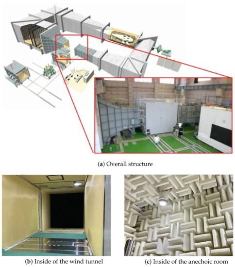
Figure 1.
JAXA’s 2 m × 2 m low-speed wind tunnel and an anechoic cart.
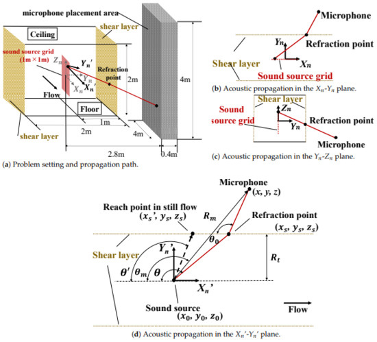
Figure 2.
Schematic image of acoustic propagation.

Table 1.
The flow velocity and the microphone placement area to be analyzed.
3. Calculation of Propagation Time and Attenuation Rate Using the Amiet Method
This section explains the calculation method of the propagation time and the attenuation rate considering the effect of the refraction at the shear layer. Here, the Amiet method [5,12], which is a de facto standard method calculating the refraction in geometric acoustics, is employed, and the effects of the refraction on the acoustic waves are considered.
As mentioned in the problem setting of the present study, we consider the propagation time and attenuation rate from one microphone to grid points in the sound source localization area. The propagation path from the microphone to the source grid is equivalent, even if the sound source and microphone are exchanged in their places. Thus, the propagation time and attenuation rate can be calculated by considering those of the acoustic wave that is generated from a virtual sound source located at a given grid point. Figure 2a–c show a schematic image of the propagation path when considering the acoustic wave generated from one point on the sound source grid and its refraction. The acoustic propagation actually occurs in a three-dimensional space, but the refraction can be considered to be two-dimensional because the flow velocity in the and axes inside the wind tunnel is zero and the air density does not change through the shear layer. Therefore, the refraction occurs in the plane, but not in the plane. The propagation, including refraction, can be assumed to only occur in the plane, as shown in Figure 2a. While Amiet derived the refraction correction formulas in the plane perpendicular to the shear layer [5,12], the present study simply extends this Amiet formula to outside the plane perpendicular to the shear layer with the assumption of the same sound speed inside and outside the test section as each other. An additional assumption simplifies the calculation. The deviation of the extended formula is presented, as follows.
3.1. Effect of the Refraction on the Propagation Path
Figure 2d shows a schematic image of the acoustic propagation in the plane. When the flow velocity in the wind tunnel is zero, acoustic waves travel along the dashed line with the propagation angle of . However, there is actually a flow in the wind tunnel and the sound wave propagation path changes, as shown by the red solid line at the propagation angle .
The geometric relationship can be derived, as shown in Figure 2d,
where , , , and are the distance from the sound source to the microphone, the distance between the sound source to the shear layer, the angle to source-microphone vector, and the angle to shear layer-microphone vector, respectively.
The relationship between and can be obtained from the convection of the acoustic wave,
where M is the Mach number of the flow.
3.2. Propagation Time
The propagation time from the sound source to the shear layer does not change, regardless of the flow velocity. This is because the and components of the flow velocity are zero, and the sound speed towards the shear layer does not change. This is based on the assumption that sound wave propagates through air as a medium and, therefore, the effective sound speed changes according to the speed of the medium. In other words, the propagated point in the shear layer is changed by the convection due to the freestream velocity under the same propagation time as that without convection.Therefore, the propagation time inside the wind tunnel is derived, as follows:
where , , and c are the positions that the sound wave reaches the shear layer without the flow velocity, the sound source position, and the sound speed, respectively. Because the sound wave is only advected in the flow direction by before reaching the shear layer, is given by Equation (5).
where is the position of the refraction in the local coordinate system. subsequently, the propagation time inside the wind tunnel is derived from Equations (4) and (5), as follows.
The propagation time outside the wind tunnel is given by the following equation:
where is the position of the microphone in the local coordinate system. Therefore, the propagation time from the sound source to the microphone is given by
3.3. Attenuation Rate
Figure 3 shows the schematic image of the acoustic rays that are emitted from the sound source with a small angle .
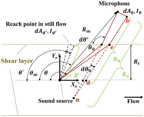
Figure 3.
The two adjacent emitted acoustic rays.
The acoustic energies that perpendicularly pass through the integration areas of and are equated, as follows:
where and are the acoustic intensities at the inside and outside wind tunnel, respectively.
3.3.1. Derivation of
The distance from the sound source to the shear layer without the flow velocity is given by the geometric relationship shown in Figure 3:
Here, can be derived when considering Equation (10).
3.3.2. Derivation of
Equation (13) can be derived from the sine formula:
where is the distance from the points a to e as shown in Figure 3. Equation (13) can be recast into Equation (14) by substituting Equation (2) into Equation (13), as follows:
Equation (3) is transformed, as follows:
Here, is the distance from the points a to d. Subsequently, is given by , as follows.
3.3.3. Derivation of and
The acoustic intensity inside the wind tunnel is defined, as follows:
On the other hand, the acoustic intensity outside the wind tunnel is defined as follows:
where , , and are the acoustic pressure at the point b, the acoustic pressure at the point e, and the density, respectively.
3.3.4. Derivation of and
Here, is given, as follows.
3.4. Distribution of Propagation Time and Attenuation Rate
Figure 4 shows the distributions of the propagation time and the attenuation rate in the plane ( = 0) calculated using the derived equations. The position of the sound source was set to be (0, 0, 0), and the Mach number inside the wind tunnel M = 0.3 and sound speed c = 340 m/s.
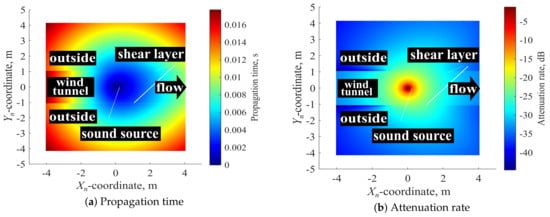
Figure 4.
The distributions of propagation time and attenuation rate in the − plane ( = 0).
The distributions of both propagation time and attenuation rate extend downstream by the convection in the wind tunnel. In addition, the attenuation rate of upstream drops significantly outside the wind tunnel by the effect of refraction at the shear layer. Therefore, the equations of the propagation time and attenuation rate are reasonable.
4. Reduction of Computational Costs with Data-Driven Sparse Sampling
The sound source localization using beamforming requires the exhaustive calculation of the propagation time and attenuation rate at each point of the sound source localization area, as described in Section 3. However, this requires high calculation costs if the number of the grid points in the source area is large, such as 200 × 200 points, as in the present study. Because the Amiet method [5] involves iterative calculations, the calculation takes approximately eight minutes for 40,000 source points of one microphone. Hundreds of microphones are sometimes used in the experiments and, therefore, the exhaustive calculation of the propagation time and the attenuation rate seems to be difficult in the online quick check of experiments. Therefore, this study proposes a reduction in the calculation cost using data-driven sparse sampling.
The data-driven sparse sampling [13] is a method for reconstructing the entire field of the high-dimensional data using a few dominant modes that are based on the modal decomposition, such as SVD.
where , , and , and are the estimated propagation time or attenuation rate distributions of 40,000 grid point, the spatial-mode matrix, and the latent-state vector (the mode coefficient), respectively. Here, r is the number of mode and p is the number of sampling points. If the spatial mode shape in is appropriately selected, then the distributions of 40,000 grid points can be expressed by a small number of latent variable. If this approximation works well, the latent variable can be determined by the observations at suboptimized sparse sampling points:
where and are the observation vector and sparse-sampling point matrix indicating the positions of p sampling points that were highly sensitive to the latent state variables. Here, is determined by the problem choosing p sampling points out of 40,000 grid points for the better estimation of the latent state variables that express the mode coefficients. The estimated mode coefficients can be obtained by multiplying the pseudo inverse matrix of , as follows.
Finally, , corresponding to the overall propagation time or attenuation rate distributions of 40,000 grid points, can be reconstructed by substituting into Equation (27).
SVD constructs the spatial mode matrix in the present study. The training data matrix that consists of the propagation time or the attenuation rate of 40,000 grid points at randomly selected 100 conditions in the range of Table 1 is constructed. Subsequently, SVD is applied to the training data matrix , of which the size is 40,000 × 100, and Equation (29) is obtained,
where the columns of and are orthogonal and called left and right singular vectors, respectively. The matrix contains decreasing nonnegative diagonal entries, called singular values. Here, is a low-dimensional description of the original data approximated with a low-rank matrix. If the r mode reconstruction is considered, then and contain the first columns of and , respectively, and contains the first block of . Subsequently, the sampling point candidate matrix becomes the spatial POD modes , and the latent state vector becomes the mode coefficients of the data matrix, respectively. In addition, is obtained using the greedy method [17], so that the determinant of the Fisher information matrix is maximized by considering as a sampling-point candidate matrix. See ref. [17] for the detailed explanation and refs. [14,21,22,23,24,25,26,27,28] for relevant techniques. Thus, the dominant modes and optimum p sampling points are determined based on the training data.
Once and are constructed, a test condition of microphone position and wind velocity from the range that is shown in Table 1 is chosen. Here, the test conditions are not included in the training data. The observation vector is constructed by calculating the propagation time or the attenuation rate of p sampling points under the test condition. Subsequently, and are quickly obtained by using Equations (27) and (29). For evaluation of the proposed method, the estimated data matrix is compared with the reference matrix, in which all of the points are exhaustively calculated by the Amiet method [5]. The reproducibility is verified by taking the relative error and calculating the average of each row.
5. Results and Discussion
Figure 5 and Figure 6 show the distributions of the propagation time and the attenuation rate under a certain test condition as an example of the sparse sampling. The test condition is randomly selected within the range of Table 1. Here, the microphone position and Mach number were set to be (x, y, z) = (1.2589, 1.9246, −1.4921) and M = 0.1827, respectively. The theoretical distributions are calculated as distributions of 40,000 points using the relationship between the sound source and microphone position using the Amiet method [5]. Figure 5b and Figure 6b show the estimated distributions when the numbers of the modes r and the sampling points p are 10. Circles in those figures show the positions of the selected sampling points. The sampling points that are determined by the sensor selection method [17] are uniformly distributed throughout, and the estimated distributions are close to the original distributions well. Therefore, the proposed method was found to effectively reproduce the distribution with a limited number of sampling points. Table 2 shows the computational environment.
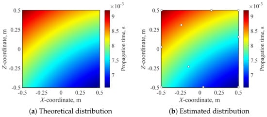
Figure 5.
Distributions of propagation time in the sound source grid.

Figure 6.
Distributions of attenuation rate in the sound source grid.
Table 2.
Computational environment.
The numbers of the modes r and the sampling points p for constructing a reduced-order model are significant parameters of the present method, because these values control the degree of freedom for expressing the original large-scale data. In this study, was estimated both when the number of sampling points was equal to the number of modes and when it was twice the number of modes
.
The proposed method estimates the amplitude of the modes using the spatial modes and the sampling points that were obtained from the training data, and it reconstructs the distributions. On the other hand, as a more conventional reconstructing method, there is a method of linearly interpolating the values between the sampling points. Therefore, the values of each sampling point selected by the sensor selection method [17] were linearly interpolated and reconstructed, and the distributions of 40,000 points are compared with the proposed method. The inverse distance weighted (IDW) interpolation [29] and triangulated irregular network (TIN) interpolation methods [30] are used for the spatial linear interpolation method. The IDW interpolation method calculates the interpolated values by a linear combination of each sampling point and its weight that reflects the shortest distance between the interpolated point and the sampling point [29]. In addition, the TIN interpolation method divides the space into multiple triangles that are based on the sampling points and calculates the interpolated values using three sampling points at the vertices of each triangle [30].
The estimation accuracy of the proposed method was evaluated using test cases, in which 50 patterns were randomly selected from the range shown in Table 1. The spatial average of relative error in each mode is defined for the quantitative evaluation, as follows:
Here, is a vector of reconstructed results that correspond to the propagation time or the attenuation rate of 40,000 grid points in the source grid. In addition, is a vector of reference values for those at each test condition. The reference values can be obtained by the exhaustive calculation of the Amiet method [5] without using sparse sampling. Figure 7 shows a comparison of the estimation accuracy of the four methods. The solid line shown in Figure 7 depicts the average of 50 test cases, and the shaded region shows the error bar defined by the minimum and maximum values of them. The calculations of the TIN interpolation methods for one to four modes are not conducted because the number of sampling points that can divide into triangles is five or more in the TIN interpolation method [30].
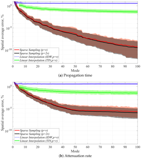
Figure 7.
Spatial average of relative error for each number of modes. Here, shaded region shows the range from the minimum to maximum values obtained for 50 runs with different random seeds.
Figure 7 shows that the error of the proposed method is significantly smaller than that of the conventional linear interpolation methods (IDW and TIN interpolation methods). The error for the case with a doubled number of sampling points (p = 2r) in the present method was found to be slightly smaller than that of p = r in the present method. Although the estimation accuracy is improved by increasing the number of sampling points, its improvement is limited in the present problem setting. The error in the propagation time monotonically decreases with increasing the number of modes from one to 100. Although the error in the attenuation rate also decreases with increasing the number of modes from 1 to 100, it does not significantly decreases after 50 modes.
The relationship between the calculation time and estimation error is discussed, and the practicality of this method for the onsite quick check in the aeroacoustic wind tunnel test is evaluated. Although the required calculation time and permissible errors are dependent on the test conditions and test campaign, a quantitative permissive error is defined based on the experience of the present authors. If the error of the propagation time exceeds one corresponding to five degrees in the phase of the target frequency, the error of sound source position that is estimated by beamforming is considered to become large in the present problem setting. These permissible errors are s, s, and s for the target frequencies of 1000 Hz, 10,000 Hz, and 100,000 Hz, respectively. Figure 8 shows plots of the spatial average of the absolute error and the calculation time for each number of modes for the reconstruction when the number of sampling points is the same as the of modes. The solid line shown in Figure 8 depicts the average of 50 test cases, and the shaded region shows the error bar that is defined by the minimum and maximum values of them, similar to those in Figure 7. The spatial average of the absolute error in each mode for the reconstruction is defined, as follows:
where N is the number of dimensions for the reconstructed fields and in this study. Figure 8 illustrates that 10 modes are considered to be an appropriate number of modes. Therefore, the condition with 10 modes is adopted, and the acceleration of the calculation time, which is one of the crucial objectives of the present study, is evaluated. The calculation time for the cases with 10 modes is 0.5936 and 0.5836 s for the propagation time and attenuation rate, respectively. On the other hand, the times for the exhaustive calculation of all 40,000 grid points by the Amiet method [5] are 376.804 and 381.793 s for the propagation time and the attenuation rate, respectively. Thus, the calculation time was greatly reduced by the proposed method as compared with the exhaustive calculation of the steering vector by the Amiet method, as we expected. Table 3 presents the summarized results.

Figure 8.
Spatial average of absolute error and calculation time (p = r). Here, the shaded regions of spatial averaged absolute error shows the range from the minimum to maximum values obtained for 50 runs with different random seeds. Shaded regions of calculation time shows the standard deviation obtained for 50 runs.
Table 3.
Comparison of calculation time.
Finally, Figure 9, Figure 10 and Figure 11 show the spatial distribution of the relative error of the proposed method, the IDW interpolation method, and the TIN interpolation method, respectively. Note that all of the results are reconstructed using 10 modes, and the calculation times of those methods are almost the same as the data-driven sparse sampling method, because the calculation time of the Amiet method is dominant. The microphone position and Mach number of this test condition were set to be (x, y, z) = (1.2589, 1.9246, −1.4921) and M = 0.1827. Although the relative error of the proposed method tends to be locally high in the regions where the sampling points are not located, the spatial averaged error is % for the propagation time, and % for the attenuation rate, respectively. In addition, the maximum error is suppressed to % for the propagation time and % for the attenuation rate, respectively. Table 4 presents the averaged error of those methods. These errors of the proposed method are much smaller than those of the IDW and TIN interpolation methods. Thus, the proposed method can be concluded to reduce the calculation cost while minimizing the estimation error when compared with conventional interpolation methods.It should be noted that the error cannot be perfectly removed, even in the proposed method, and the steering vector might be exhaustively calculated by the Amiet method for more accurate process of the experimental data after the experiments.

Figure 9.
Distributions of error in the sound source grid estimated by sparse sampling(p = r, 10 sampling points).
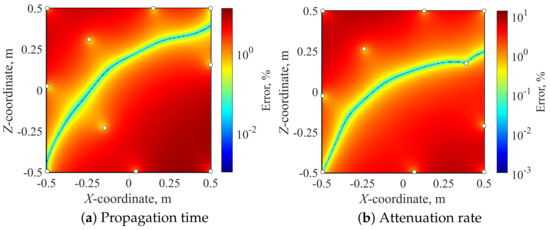
Figure 10.
Distributions of error in the sound source grid estimated by IDW interpolation (p = r, 10 sampling points).
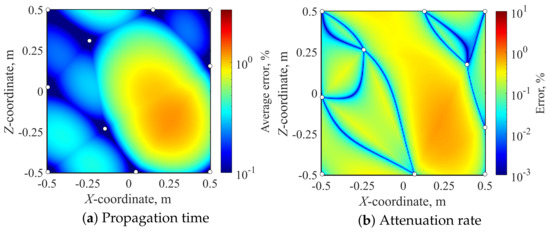
Figure 11.
Distributions of error in the sound source grid estimated by TIN interpolation (p = r, 10 sampling points).
Table 4.
A comparison of estimation error compared with the reference values.
6. Conclusions
This study proposed a high-speed algorithm for the calculation of the propagation time and attenuation rate distributions of the acoustic waves, which is applicable to onsite quick check of the aeroacoustic measurement in wind tunnel testing. Firstly, the propagation time and attenuation rate distributions, including the refraction of sound by the shear layer, were calculated over 100 patterns of combinations of the wind speed and the microphone position as training data. Subsequently, the data-driven sparse sampling was applied to these training data, and dominant modes and optimum sampling points were discovered. The reconstructed propagation time and attenuation rate distributions can be quickly calculated at sparse points of the sound source localization area. The error of the reconstructed result is 1% or less and significantly smaller than that of the conventional interpolation methods, and the calculation time is 1 s or less. In other words, the proposed method can significantly reduce the computational time of the steering vector in the onsite quick check of the experiment with minimizing the error. Therefore, the proposed method is concluded to be an onsite powerful tool for the aeroacoustic measurement in wind tunnel testing.
In the future, we will focus on the training data dependency of the data-driven sparse sampling, and we would like to enable more accurate calculations with low computational cost.
Author Contributions
S.K., K.N., Y.S. and T.N. developed the computational codes. S.K. performed the numerical experiments under the guidance of Y.O. and T.N. S.K. analyzed the data under the guidance of Y.O., T.N., Y.S., T.N. and H.U. contributed to the data interpretation. S.K., Y.O., K.N., Y.S., T.N. and K.A. contributed to writing the manuscript. All authors have read and agreed to the published version of the manuscript.
Funding
The present work was supported by the Japan Society for the Promotion of Science KAKENHI (No. 19H00800), CREST(JPMJCR1763), and ACTX(JPMJAX20AD) of Japan Science and Technology Agency.
Conflicts of Interest
The authors declare no conflict of interest.
References
- Sijtsma, P. Acoustic Array Corrections for Coherence Loss Due to The Wind Tunnel Shear Layer. In Proceedings of the 2nd Berlin Beamforming Conference, Berlin, Germany, 19–20 February 2008; GFaI, Gesellschaft zur Förderung angewandter Informatik e.V.: Berlin, Germany, 2008. [Google Scholar]
- Bahr, C.; Zawodny, S.N.; Yardibi, T.; Liu, F.; Wetzel, D.; Bertolucci, B.; Cattafesta, L. Shear Layer Correction Validation Using a Non-Intrusive Acoustic Point Source. In Proceedings of the 16th AIAA/CEAS Aeroacoustics Conference, AIAA Paper 2010–3735, Stockholm, Sweden, 7–9 June 2010. [Google Scholar] [CrossRef]
- Bahr, C.; Zawodny, S.N.; Bertolucci, B.; Li, J.; Sheplak, M.; Cattafesta, N.L. A Plasma-based Non-intrusive Point Source for Acoustic Beamforming Applications. J. Sound Vib. 2015, 344, 59–80. [Google Scholar] [CrossRef]
- Ernst, D.; Spehr, C.; Berkefeld, T. Decorrelation of Acoustic Wave Propagation through the Shear Layer in Open Jet Wind Tunnel. In Proceedings of the 21st AIAA/CEAS Aeroacoustics Conference, AIAA Paper 2015–2976, Dallas, TX, USA, 22–26 June 2015. [Google Scholar] [CrossRef]
- Allen, C.S.; Blake, W.K.; Dougherty, R.P.; Lynch, D.; oderman, R.T.; Underbrink, J.R.; Mueller, T.J. Aeroacoustic Measurements; Springer: New York, NY, USA, 2010. [Google Scholar]
- Brooks, T.F.; Humphreys, W.M. A deconvolution approach for the mapping of acoustic sources (DAMAS) determined from phased microphone arrays. J. Sound Vib. 2006, 294, 856–879. [Google Scholar] [CrossRef]
- Dougherty, R. Extensions of DAMAS and benefits and limitations of deconvolution in beamforming. In Proceedings of the 11th AIAA/CEAS Aeroacoustics Conference, Monterey, CA, USA, 23–25 May 2005; p. 2961. [Google Scholar]
- Suzuki, T. L1 generalized inverse beam-forming algorithm resolving coherent/incoherent, distributed and multipole sources. J. Sound Vib. 2011, 330, 5835–5851. [Google Scholar] [CrossRef]
- Leclere, Q.; Pereira, A.; Bailly, C.; Antoni, J.; Picard, C. A unified formalism for acoustic imaging based on microphone array measurements. Int. J. Aeroacoustics 2017, 16, 431–456. [Google Scholar] [CrossRef]
- Merino-Martínez, R.; Sijtsma, P.; Snellen, M.; Ahlefeldt, T.; Antoni, J.; Bahr, C.J.; Blacodon, D.; Ernst, D.; Finez, A.; Funke, S.; et al. A review of acoustic imaging methods using phased microphone arrays. CEAS Aeronaut. J. 2019, 10, 197–230. [Google Scholar] [CrossRef]
- Chiariotti, P.; Martarelli, M.; Castellini, P. Acoustic beamforming for noise source localization–Reviews, methodology and applications. Mech. Syst. Signal Process. 2019, 120, 422–448. [Google Scholar] [CrossRef]
- Amiet, R.K. Correction of Open Jet Wind Tunnel Measurements for Shear Layer Refraction. In Proceedings of the 2nd Aeroacoustics Conference, AIAA Paper 75–532, Hampton, VA, USA, 24–26 March 1975. [Google Scholar] [CrossRef]
- Brunton, S.L.; Kutz, J.N. Data-Driven Science and Engineering; Cambridge University Press: Cambridge, UK, 2019; Chapter 3–21. [Google Scholar]
- Manohar, K.; Brunton, B.W.; Kutz, J.N.; Brunton, S.L. Data-driven sparse sensor placement for reconstruction: Demonstrating the benefits of exploiting known patterns. IEEE Control Syst. Mag. 2018, 38, 63–86. [Google Scholar] [CrossRef]
- Drmac, Z.; Gugercin, S. A new selection operator for the discrete empirical interpolation method—improved a priori error bound and extensions. SIAM J. Sci. Comput. 2016, 38, A631–A648. [Google Scholar] [CrossRef]
- Chaturantabut, S.; Sorensen, D.C. Nonlinear model reduction via discrete empirical interpolation. SIAM J. Sci. Comput. 2010, 32, 2737–2764. [Google Scholar] [CrossRef]
- Saito, Y.; Nonomura, T.; Yamada, K.; Asai, K.; Sasaki, Y.; Tsubakino, D. Determinant-based Fast Greedy Sensor Selection Algorithm. arXiv 2019, arXiv:1911.08757. [Google Scholar]
- Loiseau, J.C.; Noack, B.R.; Brunton, S.L. Sparse reduced-order modelling: Sensor-based dynamics to full-state estimation. J. Fluid Mech. 2018, 844, 459–490. [Google Scholar] [CrossRef]
- Kanda, N.; Nakai, K.; Saito, Y.; Nonomura, T.; Asai, K. Feasibility Study on Real-time Observation of Flow Velocity Field by Sparse Processing Particle Image Velocimetry. Trans. Japan Soc. Aeronaut. Space Sci. 2019. [Google Scholar]
- Inoue, T.; Matsuda, Y.; Ikami, T.; Nonomura, T.; Hiroki Nagai, Y.E. Data-Driven Approach for Noise Reduction in Pressure-Sensitive Paint Data Based on Modal Expansion and Time-Series Data at Optimally Placed Points. arXiv 2021, arXiv:2103.00931. submitted. [Google Scholar]
- Clark, E.; Askham, T.; Brunton, S.L.; Kutz, J.N. Greedy sensor placement with cost constraints. IEEE Sens. J. 2018, 19, 2642–2656. [Google Scholar] [CrossRef]
- Manohar, K.; Kaiser, E.; Brunton, S.L.; Kutz, J.N. Optimized sampling for multiscale dynamics. Multiscale Model. Simul. 2019, 17, 117–136. [Google Scholar] [CrossRef]
- Clark, E.; Kutz, J.N.; Brunton, S.L. Sensor Selection With Cost Constraints for Dynamically Relevant Bases. IEEE Sens. J. 2020, 20, 11674–11687. [Google Scholar] [CrossRef]
- Clark, E.; Brunton, S.L.; Kutz, J.N. Multi-fidelity sensor selection: Greedy algorithms to place cheap and expensive sensors with cost constraints. IEEE Sens. J. 2020, 21, 600–611. [Google Scholar] [CrossRef]
- Saito, Y.; Nankai, K.; Yamada, K.; Asai, K.; Sasaki, Y.; Tsubakino, D. Data-driven Vector-measurement-sensor Selection based on Greedy Algorithm. IEEE Sens. Lett. 2020, 4. [Google Scholar] [CrossRef]
- Peherstorfer, B.; Drmac, Z.; Gugercin, S. Stability of discrete empirical interpolation and gappy proper orthogonal decomposition with randomized and deterministic sampling points. SIAM J. Sci. Comput. 2020, 42, A2837–A2864. [Google Scholar] [CrossRef]
- Nakai, K.; Yamada, K.; Nagata, T.; Saito, Y.; Nonomura, T. Effect of Objective Function on Data-Driven Greedy Sparse Sensor Optimization. IEEE Access 2021, 9, 46731–46743. [Google Scholar] [CrossRef]
- Yamada, K.; Saito, Y.; Nankai, K.; Nonomura, T.; Asai, K.; Tsubakino, D. Fast Greedy Optimization of Sensor Selection in Measurement with Correlated Noise. Mech. Syst. Signal Process. 2021, 158. [Google Scholar] [CrossRef]
- Shiode, S. Inverse Distance Weighted Method for Point Interpolation on a Network. Theory Appl. GIS 2004, 13, 33–41. [Google Scholar] [CrossRef]
- Akiyama, H. Triangulation Based Approximation Model for Agent Positioning Problem. Jpn. Soc. Artif. Intell. (JSAI) 2008, 23, 255–267. [Google Scholar]
Publisher’s Note: MDPI stays neutral with regard to jurisdictional claims in published maps and institutional affiliations. |
© 2021 by the authors. Licensee MDPI, Basel, Switzerland. This article is an open access article distributed under the terms and conditions of the Creative Commons Attribution (CC BY) license (https://creativecommons.org/licenses/by/4.0/).