An Updated Method for Stability Analysis of Milling Process with Multiple and Distributed Time Delays and Its Application

Abstract

Predicting and avoiding the onset of milling chatter are desirable to reduce its harm to machine tools, workpieces, and cutters. This paper presents an updated method to complete the stability prediction for the milling process with multiple and distributed time delays. After the dynamic of the combination milling process with variable helix cutter (VHC) and variable spindle speed (VSS) is modeled as linear delay differential equations with multiple and distributed time delays, the presented method is applied to carrying out its stability prediction for the first time. By comparing with the existing researches and time-domain simulations, the effectiveness of the presented method has been validated. The influence and feasibility of the combination process on chatter suppression are explored and investigated for the associated one- and two-degree-of-freedom systems. Results show that the application of the combination process can realize a further suppression of milling chatter in practice. It can result in nearly 2-fold as high as the minimum depth of cut for the traditional milling or VSS milling and about 1.3-fold for VHC milling for some special domain, and can respectively lead to the average increase of stable area by 30.4%, 23.5%, and 1.5% for the adopted simulations. However, consider the contribution, the combination process is actually one process in which VHC plays an absolutely leading role but VSS plays an auxiliary role, in terms of milling stability.

1. Introduction

Chatter in the machining process may cause problems such as poor workpiece quality, upset noise, increased tool wear, and continuous damage to the cutting spindle. Thus, predicting and avoiding the onset of chatter are important and desirable in practice. In the past, a large number of scholars carried out the research associated with cutting parameter optimization in machining to ensure the maximum material removal rate without chatter.

It is generally believed that one of the greatest sources of cutting chatter is the regeneration effect, where the displacement of the current and previous teeth of a cutter will change dynamically, resulting in dynamic cutting thickness and dynamic milling force with phase difference. Tobias and Fishwick [1] and Tlusty and Polacek [2] were the pioneers in researching chatter mechanisms and they determined the presence of the regeneration mechanism firstly in the 1960s. The main method to predict and control regeneration chatter is to obtain a stability lobe diagram (SLD), from which one can choose the process parameters corresponding to chatter-free cutting. Consequently, following the regeneration mechanism, great deal of investigations have been done on the stability prediction methods for cutting process, trying to obtain SLD accurately and efficiently. Some typical methods are: zeroth-order frequency-domain method proposed by Altintas and Budak [3], temporal finite element method by Bayly et al. [4], multi-frequency solution by Merdol and Altintas [5], Chebyshev polynomial approximation by Butcher and Bobrenkov [6], semi-discretization method (SDM) by Insperger and Stepan [7,8,9], Galerkin projection by Olgac et al. [10], Lambert W function based method by Yi and Nelson [11], Homotopy perturbation method(HPM) by He [12], Chebyshev collocation method (CCM) by Butcher et al. [13], full-discretization method (FDM) by Ding et al. [14] and Liu et al. [15], implicit subspace iteration by Zatarain et al. [16], spectral element method by Khasawneh et al. [17] and Lehotzky et al. [18], etc. Compeán et al. [19] and Sosa et al. [20] conducted the stability analysis of a multivariable milling tool by enhanced multistage HPM and high-order HPM, respectively. Urbikain et al. use CCM to deal with the turning stability prediction considering the cases with regard to the flexible workpiece [21], the slender tools [22], the large horizontal lathes [23], or the low rotational speeds [24]. Olvera et al. [25,26] made a comparison of SDM, FDM, CCM, and HPM in terms of accuracy and computational time and pointed out that CCM and HPM are the most efficient methods. Pimenov et al. [27] experimentally investigated the influence of the relative position of the face milling tool towards the workpiece on milling dynamics. Recently, Urbikain et al. [28] reviewed the current state of research with respect to the prediction methods and experimental techniques for chatter avoidance in turning in detail.

Generally, the dynamics of tool–workpiece system in milling process, considering regeneration effect, can be modeled by linear delay-differential equations (DDEs) theoretically. With the change of milling cutter style, milling strategy, actual milling conditions, and other factors in the milling process or the consideration of modeling complexity, the time-delay term in system equation changes from single one to multiple ones, to single variable one, to multiple variable ones, to distributed ones or to other forms. For instance, to deal with the problems of stability prediction for the milling with variable pitch cutter (VPC)/cutter runout [29] where the difference of the passing time between two continuous teeth leads to the existence of multiple time delays, different versions of SDM methods [30,31,32,33,34] have been put forward and their effectiveness is verified too. For predicting/optimizing the stability for milling processes with variable helix cutter (VHC) or serrated cutter characterized by the distributed delays, Sims et al. [35,36], Dombovari et al. [37,38], and Jin et al. [39] also presented suitable methods, based on SDM. It should be noted that the uses of VPC, VHC and serrated cutter are three typical methods that affect the time delay characteristics of milling process by changing the tool structure, and then suppress chatter by disturbing the regeneration effect. Another similar method is variable spindle speed (VSS), whose corresponding milling system can be expressed as the DDEs with time-dependent time delays. Around the theme of VSS, Insperger and Stepan [40], Zatarain et al. [41], Long and Balachandran [42], Seguy et al. [43], and Xie et al. [44] respectively used the updated SDM to carry out the associated stability analysis. Totis et al. [45] utilized CCM to obtain SLDs for milling process with VSS efficiently. Urbikain et al. [46] developed a stability model of VSS turning based on perturbation theory and conducted a study of its real implementation in turning systems. Bediaga et al. [47,48] studied the effectiveness of the continuous VSS with different waveforms on chatter suppression in the milling process, based on improved SDM and experimental tests.

Recently, based on SMD, Jin et al. [49,50], Zhang et al. [51] and Yang and Huang [52] investigated the milling dynamics of the combination process with VPC and VSS (or called VPCVSS), which was modeled by the DDEs with multiple and time-periodic delays. They pointed out the effectiveness of this combination for further suppression of cutting chatter. However, it should be noted that the VPC in above system, obviously, can be replaced by a VHC in practice [49], so the original system will change into new one with VHC and VSS (or called VHCVSS). In that case, there will be two main problems: (1) what is the suppression effect of this new process on cutting stability? (2) Due to the increase of system complexity, the model and algorithm in [49,50,51,52] would not be applicable anymore.

Based on the efficient methods in [15,32] with the local discretization error $\mathcal{O}(\Delta t^3)$, this paper presents an updated method to analyze the stability of milling process with multiple and distributed time delays. The innovation of this paper is mainly reflected in the following points: (1) theoretically, developing the theory in [15,32] and widening its application scope for above case; (2) applying the method to dealing with the stability prediction problem with regard to a new process, i.e., VHCVSS for the first time. Obviously, the method is not only applicable to the cases associated with VPC, VHC, or VSS, but also to their combination cases, e.g., VPCVSS and VHCVSS. The rest of this paper is organized as follows: Section 2 describes the mathematical model and the method in detail; Section 3 provides the application of the presented method for one-degree-of-freedom (DOF) and 2-DOF models associated with VHCVSS; the influence of the system parameters on chatter is analyzed. Finally, the related conclusions are given.

2. Mathematical Model

Without loss of generality, the milling dynamic of the process with multiple and distributed delays, taking into account the regeneration effects, can be expressed by an n-dimensional linear DDE [7,9,32,50] as

$$\dot{\mathit{y}}(t)=\mathit{A}\mathit{y}(t)+\mathit{B}(t)\mathit{y}(t)-{\displaystyle \sum _{j=1}^N{\displaystyle {\int }_{{\alpha }_1}^{{\alpha }_2}{\mathit{C}}_j(t,\varphi )\mathit{y}(t-{\mathit{\theta }}_j(t,\varphi ))d\varphi }}$$

(1)

where ${\rm A}$ is a constant matrix, $N$ is the number of the distributed delays, and $\mathit{B}(t)$, ${\mathit{C}}_j(t,\varphi )$ and ${\mathit{\theta }}_j(t,\varphi )$ are periodic coefficient matrices that respectively satisfy $\mathit{B}(t)=\mathit{B}(t+T)$, ${\mathit{C}}_j(t)={\mathit{C}}_j(t+T)$ and ${\mathit{\theta }}_j(t,\varphi )={\mathit{\theta }}_j(t+T,\varphi )$ with the system period $T$ and j = 1,2,…, N.

Starting with the idea in Ref. [7], Equation (1) can be written in

$$\dot{\mathit{y}}(t)=\mathit{A}\mathit{y}(t)+\mathit{B}(t)\mathit{y}(t)-{\displaystyle \sum _{j=1}^N{\displaystyle \sum _{k=1}^f{\tilde{\mathit{C}}}_{j,k}(t)\mathit{y}(t-{\tilde{\mathit{\theta }}}_{j,k}(t))}}$$

(2)

where

$$\begin{array}{l}{\tilde{\mathit{C}}}_{j,k}(t)=\{\begin{array}{cc}{\displaystyle {\int }_{{\alpha }_1}^{{\alpha }_1+kh}{\mathit{C}}_j(t,\varphi )d}\varphi & k=1,2,\dots ,f-1\\ {\displaystyle {\int }_{{\alpha }_1+(f-1)h}^{{\alpha }_2}{\mathit{C}}_j(t,\varphi )d}\varphi & k=f\end{array}\\ {\tilde{\mathit{\theta }}}_{j,k}(t)=\{\begin{array}{cc}{\mathit{\theta }}_j(t,(k-\frac{1}{2})h)& k=1,2,\dots ,f-1\\ {\mathit{\theta }}_j(t,({\alpha }_2+fh-h)/2)& k=f\end{array}\end{array}$$

(3)

Firstly, one can divide the system period T into l equal parts, and obtain l number of time intervals with length $\Delta t=T/l$. Then, for the $i-\mathrm{th}$ interval $[t_i,t_{i+1}]$, the ODE can be represented as [7]

$$\dot{\mathit{y}}(t)=\mathit{A}\mathit{y}(t)+\tilde{\mathit{B}}(t)\tilde{\mathit{y}}(t)-{\displaystyle \sum _{j=1}^N{\displaystyle \sum _{k=1}^f{\widetilde{\tilde{\mathit{C}}}}_{j,k}(t)\tilde{\mathit{y}}(t-{\tilde{\mathit{\theta }}}_{j,k,i})}}.$$

(4)

where $\tilde{\mathit{B}}(t)$ and ${\widetilde{\tilde{\mathit{C}}}}_{j,k}(t)$ respectively are the linear interpolation approximations of $\mathit{B}(t)$ and ${\tilde{\mathit{C}}}_{j,k}(t)$ on boundary $t=t_i+\xi$ ($\xi \in [0,\Delta t]$), and they can be defined by

$$\begin{array}{l}\tilde{\mathit{B}}(t)=\tilde{\mathit{B}}(\xi +t_i)={\mathit{B}}_i+\frac{{\mathit{B}}_{i+1}-{\mathit{B}}_i}{\Delta t}\xi ,\\ {\widetilde{\tilde{\mathit{C}}}}_{j,k}(t)={\widetilde{\tilde{\mathit{C}}}}_{j,k}(\xi +t_i)={\tilde{\mathit{C}}}_{j,k,i}+\frac{{\tilde{\mathit{C}}}_{j,k,i+1}-{\tilde{\mathit{C}}}_{j,k,i}}{\Delta t}\xi .\end{array}$$

(5)

and the delay item ${\tilde{\theta }}_{j,k,i}$ is equal to ${\tilde{\theta }}_{j,k,i}={\displaystyle {\int }_{t_i}^{t_{i+1}}{\tilde{\theta }}_{j,k}(t)dt}/\Delta t$. When the number of intervals corresponding to ${\tilde{\theta }}_{j,k,i}$ is defined by $m_{j,k,i}=\mathrm{ceil}({\tilde{\theta }}_{j,k,i}/\Delta t)$, the time-delayed item $\tilde{\mathit{y}}(t-{\tilde{\theta }}_{j,k,i})$ in Equation (2) can be obtained by Lagrange quadratic interpolation [15,32] at node points ${\mathit{y}}_{i-m_{j,k.i}}$, ${\mathit{y}}_{i-m_{j,k,i}+1}$ and ${\mathit{y}}_{i-m_{j,k,i}+2}$, i.e.,

$$\tilde{\mathit{y}}(t-{\tilde{\theta }}_{j,k,i})=\tilde{\mathit{y}}(\xi +t_i-{\tilde{\theta }}_{j,k,i})={\mathit{L}}_{j,k,i}(\xi ){\mathit{y}}_{i-m_{j,k,i}}+{\mathit{M}}_{j,k,i}(\xi ){\mathit{y}}_{i-m_{j,k,i}+1}+{\mathit{N}}_{j,k,i}(\xi ){\mathit{y}}_{i-m_{j,k,i}+2},$$

(6)

where

$$\begin{array}{l}{\mathit{L}}_{j,k,i}(\xi )=\frac{(\xi -v_{j,k,i}\Delta t)*(\xi -v_{j,k,i}\Delta t-\Delta t)I}{2\Delta t^2},\\ {\mathit{M}}_{j,k,i}(\xi )=\frac{(\xi +w_{j,k,i}\Delta t)*(\xi -v_{j,k,i}\Delta t-\Delta t)I}{-\Delta t^2},\\ {\mathit{N}}_{j,k,i}(\xi )=\frac{(\xi -v_{j,k,i}\Delta t)*(\xi +w_{j,k,i}\Delta t)I}{2\Delta t^2},\\ w_{j,k,i}=m_{j,k,i}-{\tilde{\tau }}_{j,k,i}/\Delta t,v_{j,k,i}=1-w_{j,k,i}.\end{array}$$

(7)

Considering ${\mathit{y}}_i$, ${\mathit{y}}_{i+1}$ and the derivatives of $\mathit{y}(t)$ at $t=t_i$ and $t=t_{i+1}$, i.e.,

$$\begin{array}{l}\dot{\mathit{y}}(t_i)={\dot{\mathit{y}}}_i=\mathit{A}{\mathit{y}}_i+{\mathit{B}}_i{\mathit{y}}_i-{\displaystyle \sum _{j=1}^N{\displaystyle \sum _{k=1}^f{\widetilde{\tilde{\mathit{C}}}}_{j,k,i}\mathit{y}(t-{\tilde{\theta }}_{j,k,i})}}\\ \dot{\mathit{y}}(t_{i+1})={\dot{\mathit{y}}}_{i+1}=\mathit{A}{\mathit{y}}_{i+1}+{\mathit{B}}_{i+1}{\mathit{y}}_{i+1}-{\displaystyle \sum _{j=1}^N{\displaystyle \sum _{k=1}^f{\widetilde{\tilde{\mathit{C}}}}_{j,k,i+1}\mathit{y}(t-{\tilde{\theta }}_{j,k,i+1})}}\end{array}$$

(8)

$\tilde{\mathit{y}}(t)$ in Equation (4) can be obtained by Cubic Hermite interpolation [32]. By collating the formula, one can get the expression

$$\tilde{\mathit{y}}(t)=\tilde{\mathit{y}}(\xi +t_i)={\mathit{U}}_i(\xi ){\mathit{y}}_i+{\mathit{V}}_i(\xi ){\mathit{y}}_{i+1}+{\mathit{W}}_i(\xi ){\displaystyle \sum _{j=1}^N{\displaystyle \sum _{k=1}^f{\widetilde{\tilde{\mathit{C}}}}_{j,k,i}{\mathit{y}}_{i-m_{j,k,i}}}}+{\mathit{X}}_i(\xi ){\displaystyle \sum _{j=1}^N{\displaystyle \sum _{k=1}^f{\widetilde{\tilde{\mathit{C}}}}_{j,k,i}{\mathit{y}}_{i-m_{j,k,i}+1}}},$$

(9)

$$\begin{array}{l}{\mathit{U}}_i(\xi )=\frac{{(\xi -\Delta t)}^2((\mathit{I}+(\mathit{A}+{\mathit{B}}_i)\xi )\Delta t+2\xi \mathit{I})}{\Delta t^3},\\ {\mathit{V}}_i(\xi )=\frac{((-\mathit{A}-{\mathit{B}}_{i+1})\Delta t^2+(3\mathit{I}+(\mathit{A}+{\mathit{B}}_{i+1})\xi )\Delta t-2\xi \mathit{I}){\xi }^2}{\Delta t^3},\\ {\mathit{W}}_i(\xi )=-\frac{{(\xi -\Delta t)}^2\xi }{\Delta t^2},X_i(\xi )=-\frac{(\xi -\Delta t){\xi }^2}{\Delta t^2},\\ {\mathit{y}}_{i-m_{j,k,i}}={\mathit{L}}_{j,k,i}(0){\mathit{y}}_{i-m_{j,k,i}}+{\mathit{M}}_{j,k,i}(0){\mathit{y}}_{i-m_{j,k,i}+1}+{\mathit{N}}_{j,k,i}(0){\mathit{y}}_{i-m_{j,k,i}+2},\\ {\mathit{y}}_{i-m_{j,k,i}+1}={\mathit{L}}_{j,k,i}(\Delta t){\mathit{y}}_{i-m_{j,k,i}}+{\mathit{M}}_{j,k,i}(\Delta t){\mathit{y}}_{i-m_{j,k,i}+1}+{\mathit{N}}_{j,k,i}(\Delta t){\mathit{y}}_{i-m_{j,k,i}+2}.\end{array}$$

(10)

Taking Equations (5), (6) and (9) into Equation (4), the solution of Equation (4) with the initial condition ${\mathit{y}}_i=\mathit{y}(t_{i+1})$ can be rearranged as

$${\mathit{Q}}_{\mathit{i}}{\mathit{x}}_{i+1}={\mathit{H}}_i{\mathit{x}}_i+{\displaystyle \sum _{j=1}^N{\displaystyle \sum _{k=1}^f({\mathit{H}}_{i-m_{j,k,i}}{\mathit{x}}_{i-m_{j,k,i}}+{\mathit{H}}_{i-m_{j,k,i}+1}{\mathit{x}}_{i-m_{j,k,i}+1}+{\mathit{H}}_{i-m_{j,k,i}+2}{\mathit{x}}_{i-m_{j,k,i}+2})}}$$

(11)

where

$$\begin{array}{l}{\mathit{Q}}_i=\mathit{I}-d{\mathit{B}}_i-\tilde{d}{\mathit{B}}_{i+1},\\ {\mathit{H}}_i={\mathit{H}}_1{\mathit{B}}_i+{\mathit{H}}_2{\mathit{B}}_{i+1}+e^{\mathit{A}\Delta t},\\ {\mathit{H}}_{i-m_{j,k,i}}={\mathit{e}}_{j,k,i}{\tilde{\mathit{C}}}_{j,k,i}+{\tilde{\mathit{e}}}_{j,k,i}{\tilde{\mathit{C}}}_{j,k,i+1},\\ {\mathit{H}}_{i-m_{j,k,i}+1}={\mathit{f}}_{j,k,i}{\tilde{\mathit{C}}}_{j,k,i}+{\tilde{\mathit{f}}}_{j,k,i}{\tilde{\mathit{C}}}_{j,k,i+1},\\ {\mathit{H}}_{i-m_{j,k,i}+2}={\mathit{g}}_{j,k,i}{\tilde{\mathit{C}}}_{j,k,i}+{\tilde{\mathit{g}}}_{j,k,i}{\tilde{\mathit{C}}}_{j,k,i+1}.\end{array}$$

(12)

For ${\mathit{\Phi }}_0={\mathit{A}}^{-1}(e^{\mathit{A}\Delta t}-\mathit{I})$, ${\mathit{\Phi }}_1={\mathit{A}}^{-1}({\mathit{\Phi }}_0-\Delta tI)$, ${\mathit{\Phi }}_2={\mathit{A}}^{-1}(2{\mathit{\Phi }}_1-\Delta t^{2}I)$, ${\mathit{\Phi }}_3={\mathit{A}}^{-1}(3{\mathit{\Phi }}_2-\Delta t^{3}I)$ and ${\mathit{\Phi }}_4={\mathit{A}}^{-1}(4{\mathit{\Phi }}_3-\Delta t^{4}I)$, the matrix $d$, $\tilde{d}$, $H_1$, $H_2$, $e_{j,k,i}$, ${\tilde{e}}_{j,k,i}$, $f_{j,k,i}$, ${\tilde{f}}_{j,k,i}$, $g_{j,k,i}$ and ${\tilde{g}}_{j,k,i}$ in Equation (9) following the idea in [15] can be expressed as

$$\begin{array}{l}\mathit{d}=-(\frac{\mathit{A}}{\Delta t^3}-\frac{2I}{\Delta t^4}){\mathit{\Phi }}_4+(\frac{2\mathit{A}}{\Delta t^2}-\frac{5I}{\Delta t^3}){\mathit{\Phi }}_3+(\frac{3I}{\Delta t^2}-\frac{\mathit{A}}{\Delta t}){\mathit{\Phi }}_2,\\ \tilde{\mathit{d}}=(\frac{\mathit{A}}{\Delta t^3}-\frac{2I}{\Delta t^4}){\mathit{\Phi }}_4+(\frac{3I}{\Delta t^3}-\frac{\mathit{A}}{\Delta t^2}){\mathit{\Phi }}_3,\\ {\mathit{H}}_1=(\frac{5I}{\Delta t^3}-\frac{3\mathit{A}}{\Delta t^2}){\mathit{\Phi }}_3+{\mathit{\Phi }}_0+(\mathit{A}-\frac{I}{\Delta t}){\mathit{\Phi }}_1+(\frac{3\mathit{A}}{\Delta t}-\frac{3I}{\Delta t^2}){\mathit{\Phi }}_2-(\frac{2I}{\Delta t^4}+\frac{\mathit{A}}{\Delta t^3}){\mathit{\Phi }}_4,\\ {\mathit{H}}_2=\frac{{\mathit{\Phi }}_1}{\Delta t}+\frac{\mathit{A}{\mathit{\Phi }}_2}{\Delta t}+(-\frac{2\mathit{A}}{\Delta t^2}-\frac{3I}{\Delta t^3}){\mathit{\Phi }}_3+(\frac{2I}{\Delta t^4}+\frac{\mathit{A}}{\Delta t^3}){\mathit{\Phi }}_4,\\ {\mathit{e}}_{j,k,i}=(-1+\frac{3w_{j,k,i}}{2}-\frac{w_{j,k,i}^2}{2}){\mathit{\Phi }}_0+\frac{{\mathit{\Phi }}_3}{2\Delta t^3}+(-\frac{2}{\Delta t^2}+\frac{w_{j,k,i}}{\Delta t^2}){\mathit{\Phi }}_2+(\frac{5}{2\Delta t}-\frac{5w_{a,j}}{2\Delta t}+\frac{w_{j,k,i}^2}{2\Delta t}){\mathit{\Phi }}_1,\\ {\tilde{\mathit{e}}}_{j,k,i}=-\frac{{\mathit{\Phi }}_3}{2\Delta t^3}+(\frac{3}{2\Delta t^2}-\frac{w_{j,k,i}}{\Delta t^2}){\mathit{\Phi }}_2+(-\frac{1}{\Delta t}+\frac{3w_{j,k,i}}{2\Delta t}-\frac{w_{j,k,i}^2}{2\Delta t}){\mathit{\Phi }}_1,\\ {\mathit{f}}_{j,k,i}=-\frac{{\mathit{\Phi }}_3}{\Delta t^3}+(-2w_{j,k,i}+w_{j,k,i}^2){\mathit{\Phi }}_0+(\frac{3}{\Delta t^2}-\frac{2w_{j,k,i}}{\Delta t^2}){\mathit{\Phi }}_2+(-\frac{2}{\Delta t}+\frac{4w_{j,k,i}}{\Delta t}-\frac{w_{j,k,i}^2}{\Delta t}){\mathit{\Phi }}_1,\\ {\tilde{f}}_{j,k,i}=\frac{{\mathit{\Phi }}_3}{\Delta t^3}+(-\frac{2}{\Delta t^2}+\frac{2w_{j,k,i}}{\Delta t^2}){\mathit{\Phi }}_2+(-\frac{2w_{j,k,i}}{\Delta t}+\frac{w_{j,k,i}^2}{\Delta t}){\mathit{\Phi }}_1,\\ {\mathit{g}}_{j,k,i}=\frac{{\mathit{\Phi }}_3}{2\Delta t^3}+(\frac{w_{j,k,i}}{2}-\frac{w_{j,k,i}^2}{2}){\mathit{\Phi }}_0+(-\frac{1}{\Delta t^2}+\frac{w_{j,k,i}}{\Delta t^2}){\mathit{\Phi }}_2+(\frac{1}{2\Delta t}-\frac{3w_{j,k,i}}{2\Delta t}+\frac{w_{j,k,i}^2}{2\Delta t}){\mathit{\Phi }}_1,\\ {\tilde{\mathit{g}}}_{j,k,i}=-\frac{{\mathit{\Phi }}_3}{2\Delta t^3}+(\frac{1}{2\Delta t^2}-\frac{w_{j,k,i}}{\Delta t^2}){\mathit{\Phi }}_2+(\frac{w_{j,k,i}}{2\Delta t}-\frac{w_{j,k,i}^2}{2\Delta t}){\mathit{\Phi }}_1.\end{array}$$

(13)

Now, if defining state vector ${\mathit{V}}_i={[{\mathit{x}}_i,{\mathit{x}}_{i-1}\cdots ,{\mathit{x}}_{i-MX+1},{\mathit{x}}_{i-MX}]}^T$ with $MX=\max (m_{j,k,i})$, Equation (8) can be recast into a discrete map form [7,8,9] as

$${\mathit{V}}_{i+1}={\mathit{Z}}_i{\mathit{V}}_i$$

(14)

where ${\mathit{Z}}_i$ is the coefficient matrix in the form of

$${\mathit{Z}}_i=\left[\begin{array}{cccccc}{\mathit{Q}}_i^{-1}{\mathit{H}}_i& 0& \cdots & 0& 0& 0\\ I& 0& \cdots & 0& 0& 0\\ 0& I& \cdots & 0& 0& 0\\ ⋮& ⋮& \ddots & ⋮& ⋮& ⋮\\ 0& 0& \cdots & I& 0& 0\\ 0& 0& \cdots & 0& I& 0\end{array}\right]+{\displaystyle \sum _{j=1}^N{\displaystyle \sum _{k=1}^f\left[\begin{array}{ccccccc}0& \cdots & {\mathit{Q}}_i^{-1}{\mathit{H}}_{i-m_{j,k,i}+2}& {\mathit{Q}}_i^{-1}{\mathit{H}}_{i-m_{j,k,i}+1}& {\mathit{Q}}_i^{-1}{\mathit{H}}_{i-m_{j,k,i}}& \cdots & 0\\ 0& \cdots & 0& 0& 0& \cdots & 0\\ 0& \cdots & 0& 0& 0& \cdots & 0\\ ⋮& ⋮& ⋮& ⋮& ⋮& ⋮& ⋮\\ 0& \cdots & 0& 0& 0& \cdots & 0\\ 0& \cdots & 0& 0& 0& \cdots & 0\end{array}\right]}}$$

(15)

Through coupling the coefficient matrix ${\mathit{Z}}_i$ in Equation (15) for l continuous time intervals in the system period, the Floquet transition matrix [8,9] can be obtained approximately as

$$\mathit{\Phi }={\mathit{Z}}_{l-1}{\mathit{Z}}_{l-2}\cdots {\mathit{Z}}_1{\mathit{Z}}_0$$

(16)

Then, the eigenvalues of the transition matrix $\mathit{\Phi }$ in Equation (16) can be calculated. If all the eigenvalues are less than unity in modulus, the investigated system is stable. Otherwise, it is unstable [7].

3. Stability Analysis and Discussion

Based on the method presented in the Section 2, the cutting process stability about the process with VHCVSS will be analyzed. For the convenience of analysis, similar to the idea in [49], four kinds of cutting processes are defined at first: Process I (i.e., conventional cutting, see the combination of Figure 1a,c), Process II (i.e., the cutting with VSS, see the combination of Figure 1b,c), Process III (i.e., the cutting with VHC, see the combination of Figure 1a,e), and Process IV (the cutting with VSS and VHC, see combination of Figure 1b,e).

The main purpose, here, is as follows: (1) Apply the method proposed in this paper to above four processes, carry out the stability prediction about the corresponding 1-DOF (see Figure 2a) and 2-DOF (see Figure 2b) systems, and effectively expand the application scope of the original methods; (2) The effectiveness and feasibility of chatter suppression by the combination process with VHCVSS are explored, and its influence on cutting stability is investigated.

3.1. Single DOF Model of VHCVSS

For a milling process, when the workpiece is regarded to be significantly more flexible in comparison with the cutter [5], the vibration of the workpiece need to be considered but that of the cutter. Then, the associated system equations can be simplified and be expressed by the 1-DOF DDEs. This is more suitable for some specially situations, such as thin-wall cutting system or flexible support system.

3.1.1. Modeling

Compared with a VPC, the pitches of a VHC vary with the axial height z. Considering regeneration effect, the related time delay will be a function of z. When the effect of VSS is also taken into account, the multiple and time-varying delays ${\tau }_j(t,\varphi )$ associated with VPCVSS (for more details, see [49]) will be changed to the multiple and distributed ones ${\tau }_j(t,z)$ for VHCVSS.

Starting with this idea, considering the nonlinear force model in [7], the 1-DOF dynamic equation of a VHCVSS milling shown in Figure 2a,c, can be expressed as

$$m_x\ddot{x}(t)+c_x\dot{x}(t)+k_{x}x(t)=-{\displaystyle \sum _{j=1}^N{\displaystyle {\int }_0^{a_p}{h}_j(z,t)(x(t)-x(t-{\tau }_j(t,z)))dz}}$$

(17)

where $m_x$,$c_x=m_x{\omega }_x^2$ and $k_x=2m_x{\zeta }_x{\omega }_x$ respectively are the mode mass, the damping coefficient and the spring stiffness where ${\zeta }_x$ is the damping ratios and ${\omega }_x$ is the natural frequencies, $N$ is the number of the cutter teeth, $h_j(t,z)$ are the dynamic chip thickness for the j-th tooth defined as

$$h_j(t,z)=q{f}_z^{q-1}{g}_j(t,z){\sin }^q{\varphi }_j(t,z)(K_t\cos {\varphi }_j(t,z)+K_r\sin {\varphi }_j(t,z))$$

(18)

where $f_z$ is the feed per tooth, q is the nonlinear factor related to the milling force, $K_t$ and $K_r$ are cutting force coefficients in tangential and radial direction, the angular position for the j tooth is

$${\varphi }_j(t,z)=\{\begin{array}{c}\frac{2\pi }{60}{\displaystyle {\int }_0^t\mathsf{\Omega }(s)ds}-z\rho ,ifj=1\\ \frac{2\pi }{60}{\displaystyle {\int }_0^t\mathsf{\Omega }(s)ds}+{\displaystyle \sum _{i=2}^j{\psi }_i}-z\rho ,if1<j\le N\end{array}$$

(19)

where $\mathsf{\Omega }(s)$ is the variable spindle speed and $\rho$ is equal to $\tan {\beta }_j/R$. For a sinusoidal modulation [7] as shown in Figure 1b, the time period is $T=60/{\mathsf{\Omega }}_0/\mathrm{RVF}$, the amplitude is ${\mathsf{\Omega }}_1=\mathrm{RVA}\times {\mathsf{\Omega }}_0$ and its function can be expressed by

$$\mathsf{\Omega }(t)={\mathsf{\Omega }}_0+{\mathsf{\Omega }}_1\sin (\frac{2\pi }{T}t)={\mathsf{\Omega }}_0[1+\mathrm{RVA}\cdot \sin (\mathrm{RVF}\cdot \frac{2\pi }{60}{\mathsf{\Omega }}_{0}t)]$$

(20)

where $\mathrm{RVA}={\mathsf{\Omega }}_1/{\mathsf{\Omega }}_0$ and $\mathrm{RVF}=60/({\mathsf{\Omega }}_{0}T)$ are respectively used to characterize the ratio of the speed variation amplitude to nominal spindle speed and the ratio of the speed variation frequency to the nominal spindle speed in a VSS milling.

Considering Equations (2) and (3), and slicing the axial depth of cut into f disks axially (see Figure 3), then Equation (17) can be changed into

$$m_x\ddot{x}(t)+c_x\dot{x}(t)+k_{x}x(t)=-{\displaystyle \sum _{j=1}^N{\displaystyle \sum _{k=1}^f{\tilde{C}}_{j,k}(t)(x(t)-x(t-{\tilde{\tau }}_{j,k}(t)))}}$$

(21)

where

$$\begin{array}{l}{\tilde{C}}_{j,k}(t)=\{\begin{array}{cc}{\displaystyle {\int }_{(k-1)h}^{kh}{h}_j(z,t)d}z& k=1,2,\dots ,f-1\\ {\displaystyle {\int }_{(f-1)h}^{a_p}{h}_j(z,t)d}\varphi & k=f\end{array}\\ {\tilde{\tau }}_{j,k}(t)={\tau }_j(t,a_k)\\ a_k=\{\begin{array}{cc}(k-\frac{1}{2})h& k=1,2,\dots ,f-1\\ (a_p+fh-h)/2& k=f\end{array}\end{array}$$

(22)

In order to select the appropriate value of f to reduce the calculation cost, the values of $h$ in Equation (22) can be calculated by $2\pi R/\tan {\beta }_1/l$. Under the circumstances of VHCVSS, the time delay ${\tilde{\tau }}_{j,k}(t)$in Equation (20) can be written as

$${\displaystyle {\int }_{t-{\tilde{\tau }}_{j,k}(t)}^t\frac{\mathsf{\Omega }(s)}{60}}ds=\frac{{\tilde{\psi }}_{j,k}}{360}$$

(23)

Clearly, one cannot obtain a closed form of ${\tilde{\tau }}_{j,k}(t)$ in Equation (23), thus, only numerical calculation can be used [7]. It should be noted that because compared to ${\mathsf{\Omega }}_0$, the values of ${\mathsf{\Omega }}_1$ in Equation (20) can be small enough in practice, one can expand Equation (23) in series, and obtain the approximation of ${\tilde{\tau }}_{j,k}(t)$ (for more details, see [7,49]) as

$${\tilde{\tau }}_{j,k}(t)\approx {\tilde{\psi }}_{j,k}/\vartheta /6$$

(24)

where ${\tilde{\psi }}_{j,k}={\psi }_j-a_k{\gamma }_j/R$, ${\gamma }_j=\{\begin{array}{cc}\tan {\beta }_{j-1}-\tan {\beta }_j& 1<j\le N\\ \tan {\beta }_N-\tan {\beta }_1& j=1\end{array}$ and $\vartheta ={\mathsf{\Omega }}_0+{\mathsf{\Omega }}_1\sin ({\omega }_{m}t)$.

Let $y(t)=m_x\dot{x}(t)+m_x{\zeta }_x{\omega }_{x}x(t)$ and $x(t)={\left[\begin{array}{cc}x(t)& y(t)\end{array}\right]}^T$, the Equation (21) can be represented as

$$\dot{\mathit{x}}(t)=\mathit{A}\mathit{x}(t)+\mathit{B}(t)\mathit{x}(t)-{\displaystyle \sum _{j=1}^N{\displaystyle \sum _{k=1}^f{D}_{j,k}(t)\mathit{x}(t-{\tilde{\tau }}_{j,k}(t))}}$$

(25)

where

$\mathit{A}=\left[\begin{array}{cc}-{\zeta }_x{\omega }_x& 1/m_x\\ m_x{(\zeta {\omega }_x)}^2-m_x{\omega }_x^2& -{\zeta }_x{\omega }_x\end{array}\right],\mathit{B}(t)=\left[\begin{array}{cc}0& 0\\ -{\displaystyle \sum _{j=1}^N{\displaystyle \sum _{k=1}^f{\tilde{\mathit{C}}}_{j,k}(t)}}& 0\end{array}\right],{\mathit{D}}_{j,k}(t)=\left[\begin{array}{cc}0& 0\\ -{\tilde{C}}_{j,k}(t)& 0\end{array}\right]$.

3.1.2. Simulation and Analysis

Based on the 1-DOF model in Section 3.1.1 and the method in Section 2, the computer programs are written in MATLAB(R) 2009a (MathWorks, Natick, USA) and implemented on a personal computer (Lenovo, Beijing, China). The multi-parameters calculation corresponding to milling stability is carried out for above defined processes. Considering that the difference of each process is mainly reflected in the change of the variable speed parameters and the geometric parameters of variable helix cutter, therefore except for the core parameters, i.e., RVF and RVA parameters associated with VSS and the pitch at the end of the tool ($\mathit{\psi }$) and helix angle ($\mathit{\beta }$) parameters associated with VHC, other parameters are the same as that in [7] and remain unchanged in the subsequent calculation.

For the convenience of analysis, two related variations are defined to analyze the effect of the cutting parameters on chatter quantitatively firstly. One is the stable area ratio [49], which can be expressed by

$$\chi =\frac{A_0}{A}$$

(26)

and is applied to characterize the ratio between the stable area $A_0$ and the total area $A$ for a certain SLD. Another is the contribution factor $\kappa$ that is to measure the contribution of a certain process to Process IV. For Processes II and III, their contributions to process IV can be respectively expressed as ${\kappa }_{II}$and ${\kappa }_{III}$, and be defined by

$$\begin{array}{l}{\kappa }_{II}=\frac{\Delta {\chi }_{III}}{\Delta {\chi }_{II}+\Delta {\chi }_{III}}\\ {\kappa }_{III}=\frac{\Delta {\chi }_{II}}{\Delta {\chi }_{II}+\Delta {\chi }_{III}}\end{array}$$

(27)

with $\Delta {\chi }_{II}={\chi }_{IV}-{\chi }_{II}$ and $\Delta {\chi }_{III}={\chi }_{IV}-{\chi }_{III}$.

Figure 4 illustrates a number of SLDs corresponding to the 1-DOF systems for Processes I, II, III, and IV. Here, two different helical endmills with the number of teeth N = 4 and the diameter D = 20 mm are considered, i.e., Cutter-1: a conventional one with the pitches at the end of the tool $\mathit{\psi }$ = [90, 90, 90, 90]° and the helix angles $\mathit{\beta }$ = [30, 30, 30, 30]°, Cutter-2: a VHC with $\mathit{\psi }$ = [75, 85, 95, 105]° and $\mathit{\beta }$ = [35, 30, 35, 30]°. The material of workpieces is Al7050. The other calculation parameters are: up milling, the radial immersion ratio a_D = 0.5, the feed per tooth $f_z$ = 0.1mm, the cutting-force coefficients $K_t=1.07\times {10}^8{\mathrm{N}/\mathrm{m}}^{1+q}$ and $K_r=0.4\times {10}^8{\mathrm{N}/\mathrm{m}}^{1+q}$, the nonlinear parameter in cutting force $q$ = 0.75, the modal mass $m_x$$=3.1663$ kg, the natural frequency ${\omega }_x$ = 400 Hz and the damping ratio ${\xi }_x=0.02$. The black thin lines in Figure 4 are associated with Process I, they are the reference stability boundaries of the traditional milling with Cutter-1; the red dotted lines correspond to process III with Cutter-2; the cyan thin lines in the subgraphs (a)–(d) of Figure 4 respectively are the stability boundary of Process II with different RVF (RVF = 0.05, 0.1, 0.2, and 0.5) but the same RVA (RVA = 0.1) when Cutter-1 is used; the SLDs shown by the green thick lines are related to Process IV, who uses Cutter-2 on the basis of above Processes II. Obviously, it can be found from Figure 4 that compared to Process I, Processes II and III do lead to better milling stability gains, especially for low-speed region. Also, their corresponding values of $\chi$ are always larger (see Figure 5). The phenomena above imply the active influence of VHC or VSS on milling stability by the disruption of regeneration chatter, and they are also coincident with that in [35,36,37,38,40,41,42]. Then, Process IV is focused on. As seen from the green lines in Figure 4, Process IV almost always leads to the highest axial depth of cut for every adopted RVF. For instance, the values of absolute (minimum) depth of cut for $\mathsf{\Omega }$ = 3600 rpm in Figure 4b–d, can reach up to 5.4, 5.4, 5.5, and 6.5 mm, which are nearly 2-fold as high as these for processes I and II and are about 1.3-fold for Process III. The values of $\chi$ associated with SLDs in Figure 4 are compared and shown in Figure 5. It can be seen that Process IV could also gain the biggest $\chi$. From Process I to II to III to IV, the obtained values of $\chi$ keep increasing gradually. Compared with Processes I, II, and III, the average increases of stability region for Process IV at different RVF values are about 30.4%, 23.5%, and 1.5%, respectively. This illustrates that the application of Process IV can realize a further suppression of milling chatter.

However, it should be noted that compared with the stable region difference between Processes IV and III, the difference between Processes IV and II is more obvious. This seems indicate that although Processes II and III both play a contribution for realizing the combination effect, the contribution degree is obviously different. Figure 6 shows the contribution factors of Processes II and III to the combination effect for different RVF values, based on Equation (27). It can be seen that although the values of $\kappa$ for Process II is almost larger with the increase of RVF, Process III obviously has a greater contribution (the values of ${\kappa }_{III}$ are all greater than 85%). This seems indicate that Process III plays a more important role in affecting the cutting stability of Process IV. In other words, VHCVSS is essentially a process in which VHC plays an absolutely leading role but VSS plays an auxiliary role, in terms of cutting stability.

3.1.3. Model Verification

Here, the presented method will be verified by comparing with the existing research and time-domain simulation. In order to evaluate the effectiveness of this method, the researches associated with VSS process [7] and with the combination process of VPC and VSS [50] are taken into accout at first. If the comparisons of the stability boundaries plotted by the black lines in Figure 4 with those in Figure 5.17 in [7], and the comparisons of the stability boundaries plotted by the cyan lines in Figure 4 with those in Figure 3 in [50] are respectively carried out, one can see that the results gained by the presented method coincide well with those by the methods in [7,50]. This illustrates the applicability of the presented method for the stability prediction about Processes I and II.

For Process IV, to the knowledge of the authors, there is no reference literature at present. Thus, the time-domain simulation is mainly used to carry out the verification. In [53], authors constructed the contour plot of peak-to-peak (PTP) vibration by investigating the vibration amplitude of a cutter. In view of this, based on the method in [53], an improved time-domain program suitable for VHCVSS is proposed. It should be noted that compared with the program in [53], the one in this paper can not only consider the infulence of regeneration effect, cutter runout, multimodal of the system, loss of contact, and variable pitch/helix angles in the original method, but also that of variable spindle speed.

The top diagram of Figure 7 shows the SLDs in Figure 4d between the rotation speed $\mathsf{\Omega }$ = 1500–5000 rpm and the axial depth of cut $a_p$ = 0–14mm. The Subgraphs (a)–(d) in Figure 7 respectively show the corresponding contour plot of PTP by the time-domain method for above four processes under the same parameters. It can be seen that the stability boundaries obtained through the presented method are basically consistent with the that through time-domain method, not only for their curve shapes but also for the stability evolution trends caused by the processes differences. This implies the effectiveness of this method in predicting stability for VHCVSS milling. There are little differences between the predicting results and simulation ones. This may attribute to the fact that the presented method can not take into account the influence of loss-of-contact character on cutting stability, but the time domain method can.

3.2. 2-DOF Model of VHCVSS

For a milling process, when the contained cutter is regarded as a cantilever beam but the workpiece is assumed to be absolute rigidity, the vibration of the tool has to be considered but that of the workpiece. Then, the associated system equation can be simplified and defined by the DDE with 2-DOF. Compared with the 1-DOF system in Section 3.1, the 2-DOF one is a more universal and general expression, so more attentions are paid on it for the existing research.

3.2.1. Modeling

Mathematically, the 2-DOF model associated with VHCVSS milling process, shown in subgraphs (b) and (c) of Figure 2 can be written as

$$\left[\begin{array}{cc}{m}_x& 0\\ 0& m_y\end{array}\right]\left[\begin{array}{c}\ddot{x}(t)\\ \ddot{y}(t)\end{array}\right]+\left[\begin{array}{cc}{c}_x& 0\\ 0& c_y\end{array}\right]\left[\begin{array}{c}\dot{x}(t)\\ \dot{y}(t)\end{array}\right]+\left[\begin{array}{cc}{k}_x& 0\\ 0& k_y\end{array}\right]\left[\begin{array}{c}x(t)\\ y(t)\end{array}\right]={\displaystyle \sum _{j=1}^N{\displaystyle {\int }_0^{a_p}\left[\begin{array}{cc}-h_{xx,j}(t,z)& -h_{xy,j}(t,z)\\ -h_{yx,j}(t,z)& -h_{yy,j}(t,z)\end{array}\right]\left[\begin{array}{c}x(t)-x(t-{\tau }_j(t,z))\\ y(t)-y(t-{\tau }_j(t,z))\end{array}\right]dz}}$$

(28)

where the cutting force coefficients $h_{j,xx}(t,z)$, $h_{j,xy}(t,z)$, $h_{j,yx}(t,z)$, and $h_{j,yy}(t,z)$ can be presented by

$$\begin{array}{c}{h}_{xx,j}(t,z)=q{f}_z^{q-1}{g}_j(t,z){\sin }^q{\varphi }_j(t,z)(K_t\cos {\varphi }_j(t,z)+K_r\sin {\varphi }_j(t,z))\sin {\varphi }_j(t,z),\\ h_{xy,j}(t,z)=q{f}_z^{q-1}{g}_j(t,z){\sin }^q{\varphi }_j(t,z)(K_t\cos {\varphi }_j(t,z)+K_r\sin ({\varphi }_j(t,z))\cos {\varphi }_j(t,z),\\ h_{yx,j}(t,z)=q{f}_z^{q-1}{g}_j(t,z){\sin }^q{\varphi }_j(t,z)(-K_t\sin {\varphi }_j(t,z)+K_r\cos {\varphi }_j(t,z))\sin {\varphi }_j(t,z),\\ h_{yy,j}(t,z)=q{f}_z^{q-1}{g}_j(t,z){\sin }^q{\varphi }_j(t,z)(-K_t\sin {\varphi }_j(t,z)+K_r\cos {\varphi }_j(t,z))\cos {\varphi }_j(t,z).\end{array}$$

(29)

Denoting $M=\left[\begin{array}{cc}{m}_x& 0\\ 0& m_y\end{array}\right]$, $\mathit{C}=\left[\begin{array}{cc}{c}_x& 0\\ 0& c_y\end{array}\right]$, $\mathit{K}=\left[\begin{array}{cc}{k}_x& 0\\ 0& k_y\end{array}\right]$, $q(t)=\left[\begin{array}{c}x(t)\\ y(t)\end{array}\right]$, if the axial depth of cut is sliced, considering Equations (2), (3) and (28) will be changed into

$$\mathit{M}\ddot{\mathit{q}}(t)+\mathit{C}\dot{\mathit{q}}(t)+\mathit{K}\mathit{q}(t)=-{\displaystyle \sum _{j=1}^N{\displaystyle \sum _{k=1}^f{\mathit{D}}_{j,k}(t)(\mathit{q}(t)-\mathit{q}(t-{\tilde{\mathit{\tau }}}_{j,k}(t)))}}$$

(30)

where

$$\begin{array}{l}{\mathit{D}}_{j,k}(t)=\left[\begin{array}{cc}{\tilde{\mathit{C}}}_{xx,j,k}(t)& {\tilde{\mathit{C}}}_{xy,j,k}(t)\\ {\tilde{\mathit{C}}}_{yx,j,k}(t)& {\tilde{\mathit{C}}}_{yy,j,k}(t)\end{array}\right]\\ {\tilde{\mathit{C}}}_{(\bullet ),j,k}(t)=\{\begin{array}{cc}{\displaystyle {\int }_{(k-1)h}^{kh}{h}_{(\bullet ),j}(z,t)d}z& k=1,2,\dots ,f-1\\ {\displaystyle {\int }_{(f-1)h}^{a_p}{h}_{(\bullet ),j}(z,t)d}\varphi & k=f\end{array},(\bullet )=xx,xy,yx\mathrm{and}yy\end{array}$$

(31)

Denoting $\mathit{p}(t)=\mathit{M}\dot{\mathit{q}}+\mathit{c}\mathit{q}/2$ and $\mathit{x}(t)={\left[\begin{array}{cc}\mathit{q}(t)& \mathit{p}(t)\end{array}\right]}^T$, one can transform the 2-DOF model in Equation (28) into

$$\dot{x}(t)=\mathit{A}\mathit{x}(t)+\mathit{B}(t)x(t)-{\displaystyle \sum _{j=1}^N{\displaystyle \sum _{k=1}^f{\mathit{D}}_{j,k}(t)\mathit{x}(t-{\tilde{\tau }}_{j,k}(t))}}$$

(32)

where

$$\begin{array}{l}\mathit{A}=\left[\begin{array}{cc}-{\mathit{M}}^{-1}\mathit{C}/2& {\mathit{M}}^{-1}\\ \mathit{C}{\mathit{M}}^{-1}\mathit{C}/4-\mathit{K}& -\mathit{C}{\mathit{M}}^{-1}/2\end{array}\right],\mathit{B}(t)=\left[\begin{array}{cccc}0& 0& 0& 0\\ 0& 0& 0& 0\\ -{\displaystyle \sum _{j=1}^N{\displaystyle \sum _{k=1}^f{\tilde{\mathit{C}}}_{xx,j,k}(t)}}& -{\displaystyle \sum _{j=1}^N{\displaystyle \sum _{k=1}^f{\tilde{\mathit{C}}}_{xy,j,k}(t)}}& 0& 0\\ -{\displaystyle \sum _{j=1}^N{\displaystyle \sum _{k=1}^f{\tilde{\mathit{C}}}_{yx,j,k}(t)}}& -{\displaystyle \sum _{j=1}^N{\displaystyle \sum _{k=1}^f{\tilde{\mathit{C}}}_{yy,j,k}(t)}}& 0& 0\end{array}\right]\\ {\mathit{D}}_{j,k}(t,z)=\left[\begin{array}{cccc}0& 0& 0& 0\\ 0& 0& 0& 0\\ {\tilde{\mathit{C}}}_{xx,j,k}(t)& {\tilde{\mathit{C}}}_{xy,j,k}(t)& 0& 0\\ {\tilde{\mathit{C}}}_{yx,j,k}(t)& {\tilde{\mathit{C}}}_{yy,j,k}(t)& 0& 0\end{array}\right]\end{array}$$

(33)

3.2.2. Simulation and Analysis

Here, multi-parameters calculation for the milling stability of Processes I, II, III, and IV, is carried out based on the two DOF model in Section 3.2.1 and the method in Section 2. Similar to the situation in Section 3.1.2, the other parameters in the subsequent calculation remain unchanged except for the core parameters RVF, RVA, $\mathit{\psi }$, and $\mathit{\beta }$. The mainly parameters are selected from the representative papers [54], and are: down milling, half immersion, $q=1$, $K_r$ = $2.56\times {10}^8\mathrm{N}/\mathrm{m}$, $K_t$ = $6.79\times {10}^8\mathrm{N}/\mathrm{m}$, $N$ = 4, $f_z$ = 0.1 mm, ${\omega }_x$ = 563.6 Hz, ${\omega }_y$ = 516.21 Hz, ${\zeta }_x$ = 0.0558, ${\zeta }_y$ = 0.025, $m_x$ = 1.4986 kg, and $m_y$ = 1.199 kg.

Figure 8 shows some SLDs corresponding to the 2-DOF systems for Processes I, II, III, and IV. The black thin lines are the stability boundaries corresponding to Process I for reference, whose core parameters are: RVF = 1, RVA = 0, $\mathit{\psi }$ = [90, 90, 90, 90]° and $\mathit{\beta }$ = [30, 30, 30, 30]°. The cyan thin lines are related to the stability boundaries of Process II with RVF = 0.5, RVA = 0.1 and the same $\mathit{\psi }$ and $\mathit{\beta }$ in Process I. The boundaries plotted by red dotted lines in Figure 8a–d are associated with Process III, where four VHCs with the different $\mathit{\beta }$ ($\mathit{\beta }$ = [30, 30, 30, 30]°, $\mathit{\beta }$ = [32, 30, 32, 30]°, $\mathit{\beta }$ = [34, 30, 34, 30]°, and $\mathit{\beta }$ = [36, 30, 36, 30]°) but the same $\mathit{\psi }$ ($\mathit{\psi }$ = [75, 85, 95, 105]°) are utilized. The green thick lines exhibit the SLDs related to Process IV for the relevant parameters combinations of Process II and Process III. Comparing with the curves in the Figure 8, it can be found that the combined process (i.e., Process IV) still shows a better cutting stability suppression advantage than that of Processes I, II, and III. For different combinations of variable helix angles $\mathit{\beta }$, the values of $\chi$ associated with Process IV are the biggest (see Figure 9). For Process IV, the values of $\chi$ will increase for a bigger helix angle increment $\Delta \beta$ (defined by ${\mathit{\beta }}_1-{\mathit{\beta }}_2$). This shows that the increasing of $\Delta \beta$ plays a positive role in enhancing the stability area for VHCVSS. Thus, a bigger $\Delta \beta$ should be suggested in practice.

Figure 10 shows the contribution factor diagram of Processes II and III to Process IV under different $\mathit{\beta }$. Obviously, the corresponding values of ${\kappa }_{III}$ are all greater than 61%, Process III still has a significant advantage in the contribution of the combination effect, compared to Process II. However, it should be noted that the contribution factor changed most significantly when the variable helix angles change from $\mathit{\beta }$ = [30, 30, 30, 30]° to $\mathit{\beta }$ = [32, 30, 32, 30]°. This is mainly due to the fact that the former actually constructs a VPC milling process that is consistent with the model described in [49], while the latter is a VHC one. In comparison, variable helix characteristics of a VHC aggravate the degree of regeneration disturbance, and thus relatively weaken the stability influence ability of VSS in the combination process.

4. Conclusions

This paper presents an improved method to gain the SLDs for milling process with multiple and distributed time delays. After the milling dynamic of the VHCVSS process, taking into account regeneration effect, is modeled by linear DDEs with multiple and distributed time delays, the presented method is applied to deal with the problems about the stability prediction for VHCVSS process for the first time. By comparing with the existing research and time-domain simulations, the presented method has been validated. The effectiveness and feasibility of chatter suppression by the combination of VHC and VSS milling are explored and investigated for associated 1- and 2-DOF systems. Moreover, the following conclusion can be drawn:

(1)

The presented method is effective for obtaining the SLDs for milling processes with multiple and distributed time delays. Thus, the theory in [15,32] is developed and its application scope is widened.

(2)

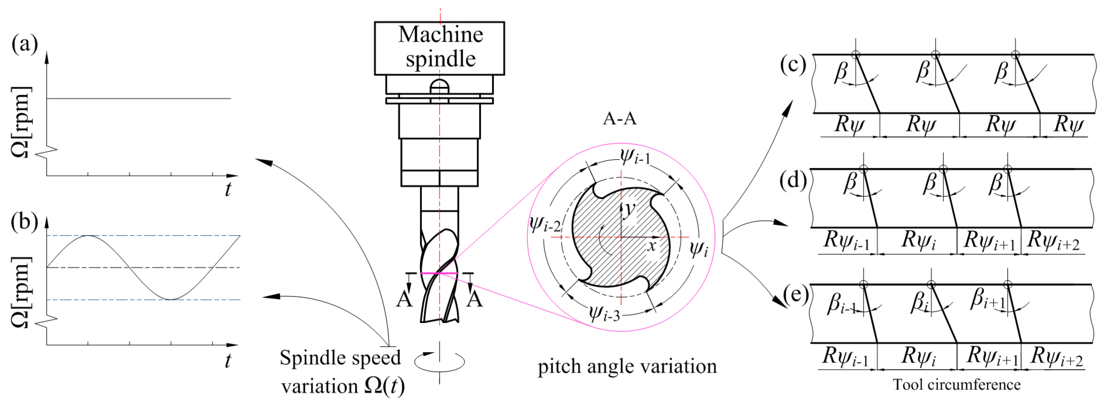
The presented method is applied to dealing with the stability prediction problem with regard to the new process, i.e., VHCVSS for the first time. Obviously, the method is not only applicable to the cases associated with VPC, VHC, or VSS, but also to their combination cases, e.g., VPCVSS and VHCVSS.

(3)

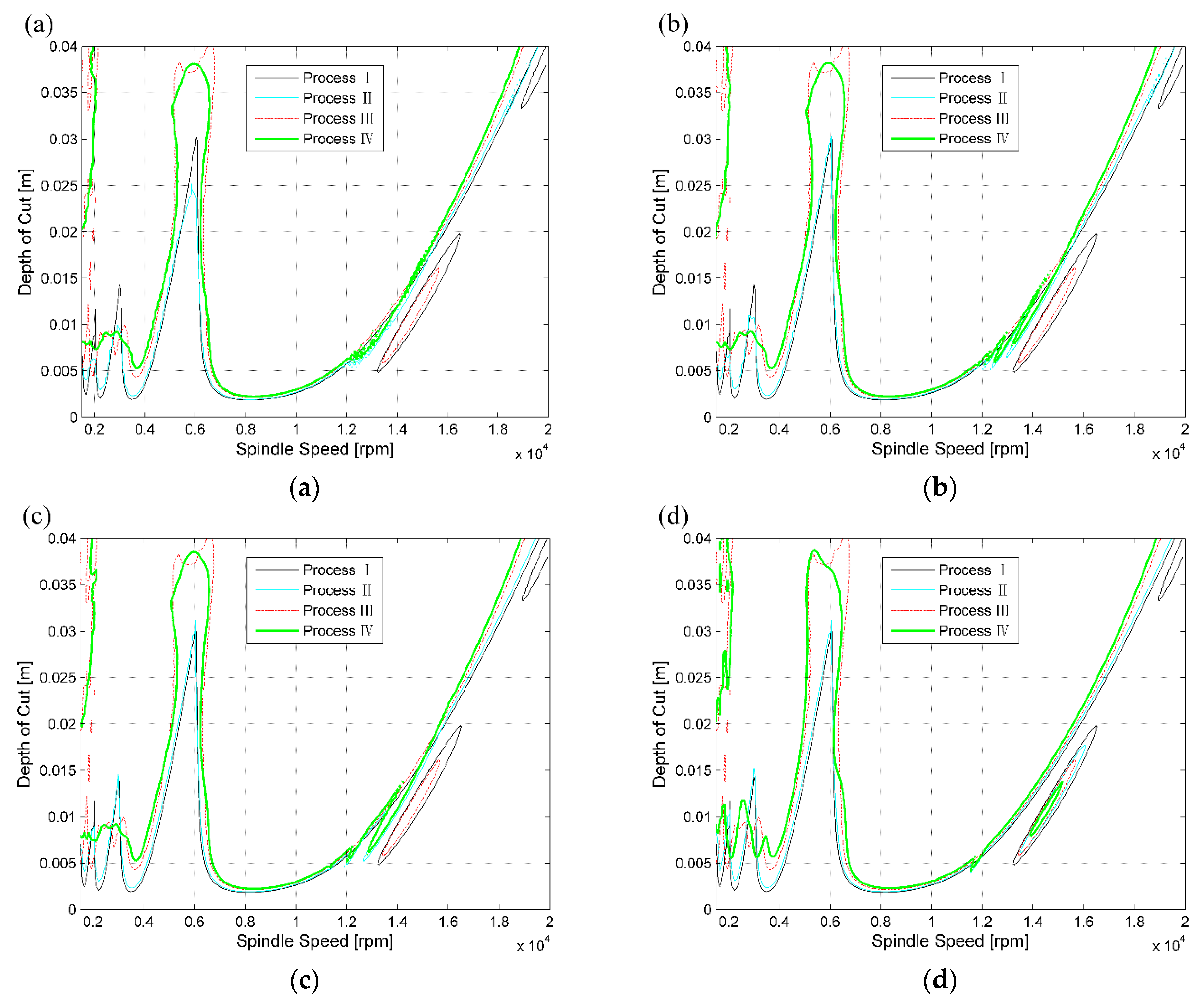
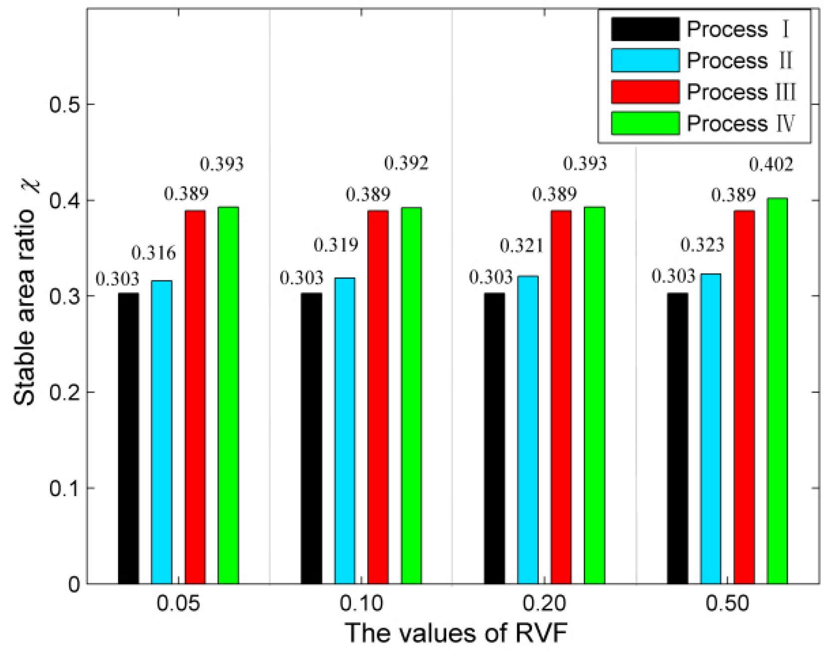
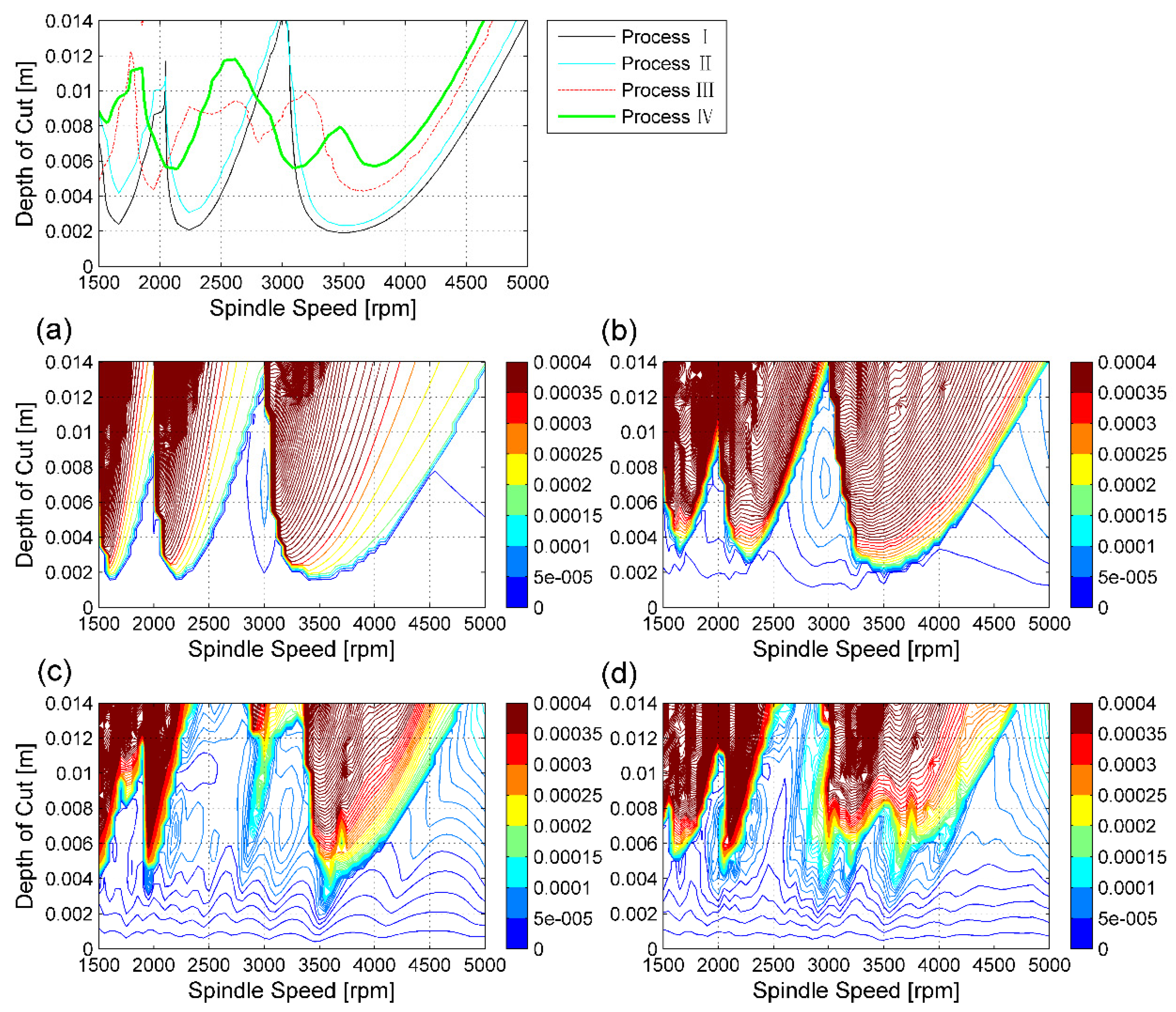
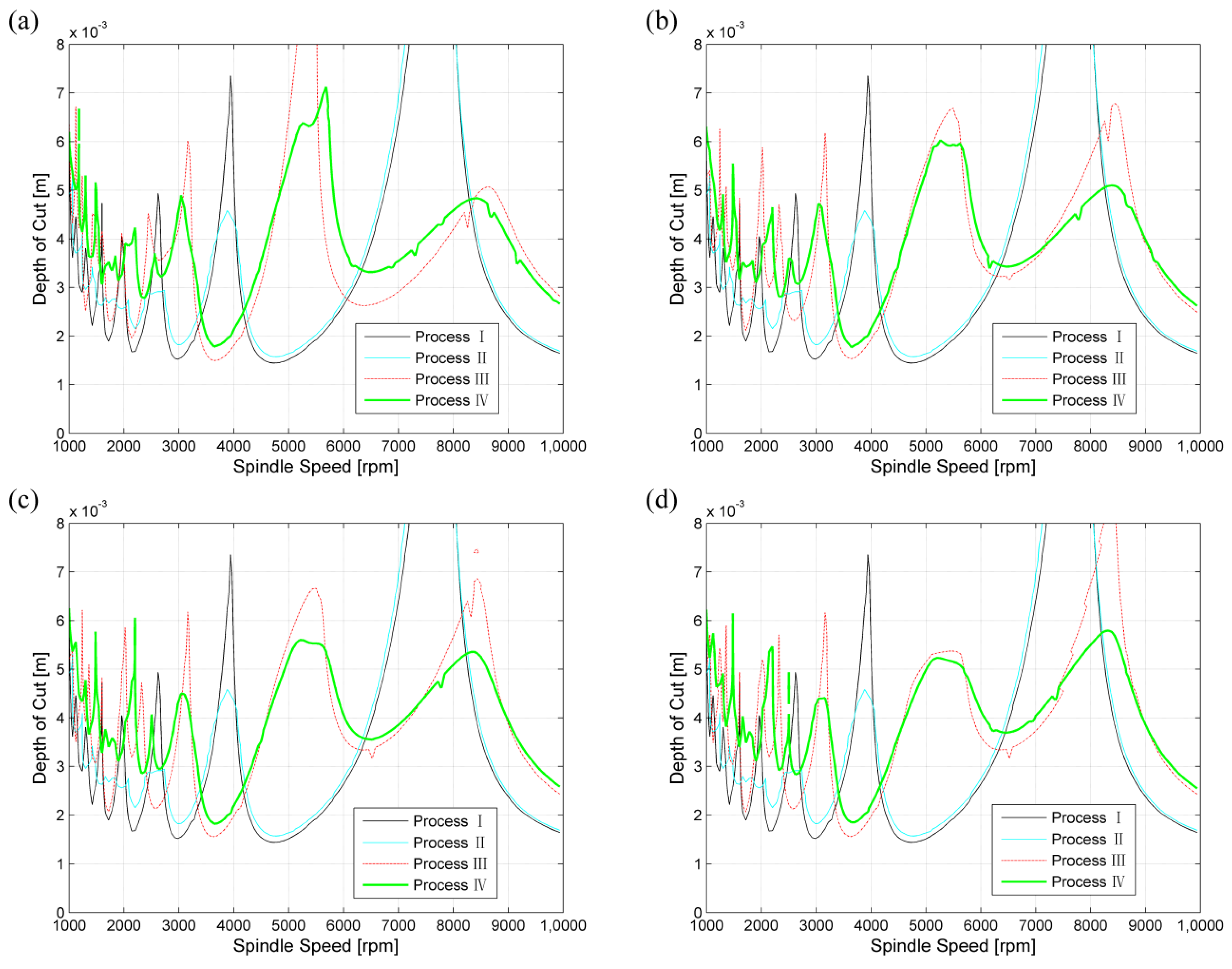
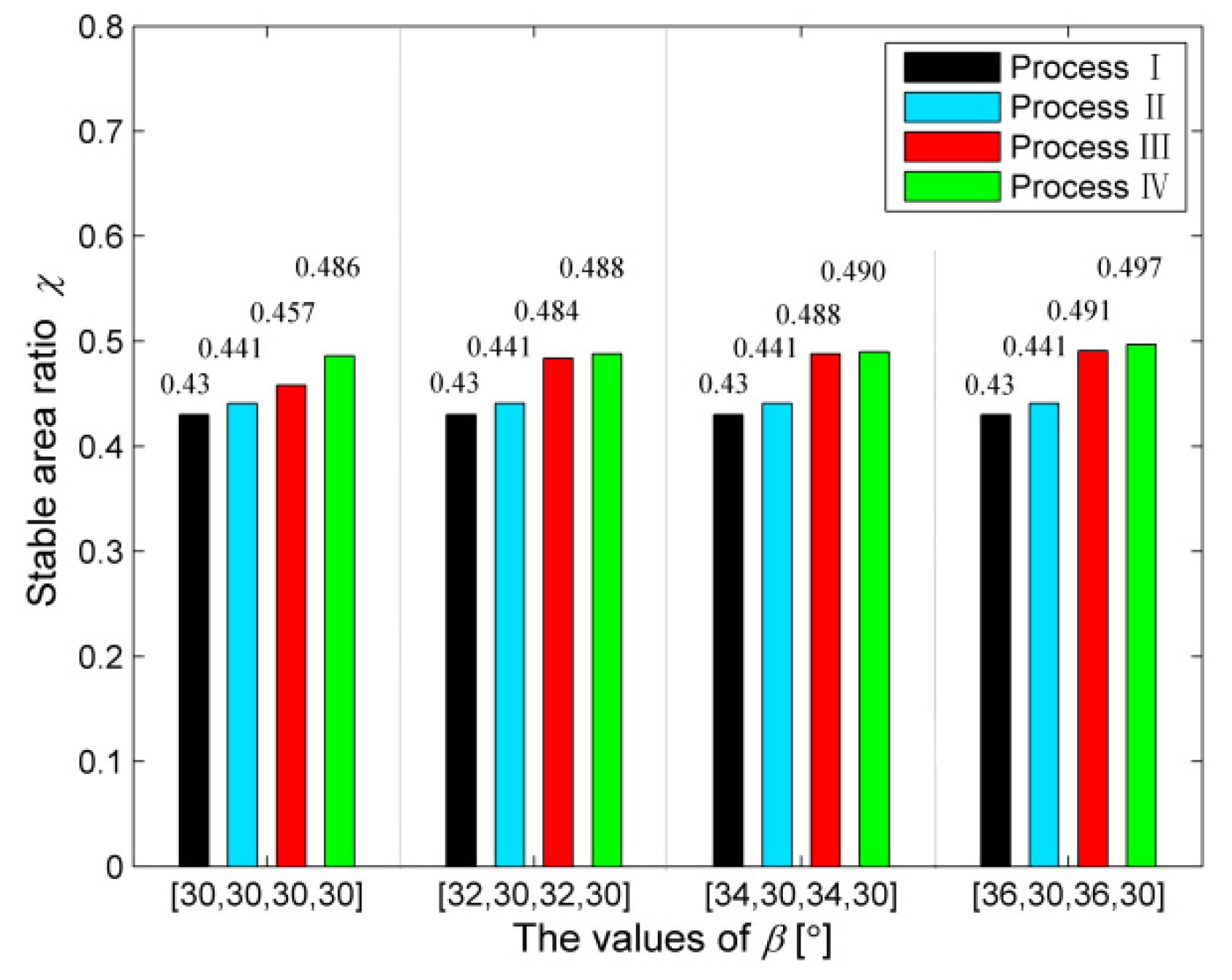
Compared with Processes I, II, and III, application of Process IV can result in nearly 2-fold as high as the minimum depth of cut for Processes I and II and are about 1.3-fold for Process III for some special domain, and can respectively lead to the average increases of stable area by 30.4%, 23.5%, and 1.5% at different RVF values. This indicates that one can improve the chatter suppression performance of the cutting system through VHCVSS in practice. The proposed method can also provide a good help for the subsequent process optimization to achieve the chatter-free maximum removal rate.

(4)

For Process IV, the increasing of the helix angle increment $\Delta \beta$ plays a positive role in enhancing the stability area for VHCVSS. Thus, bigger values of $\Delta \beta$ should be suggested in practice.

(5)

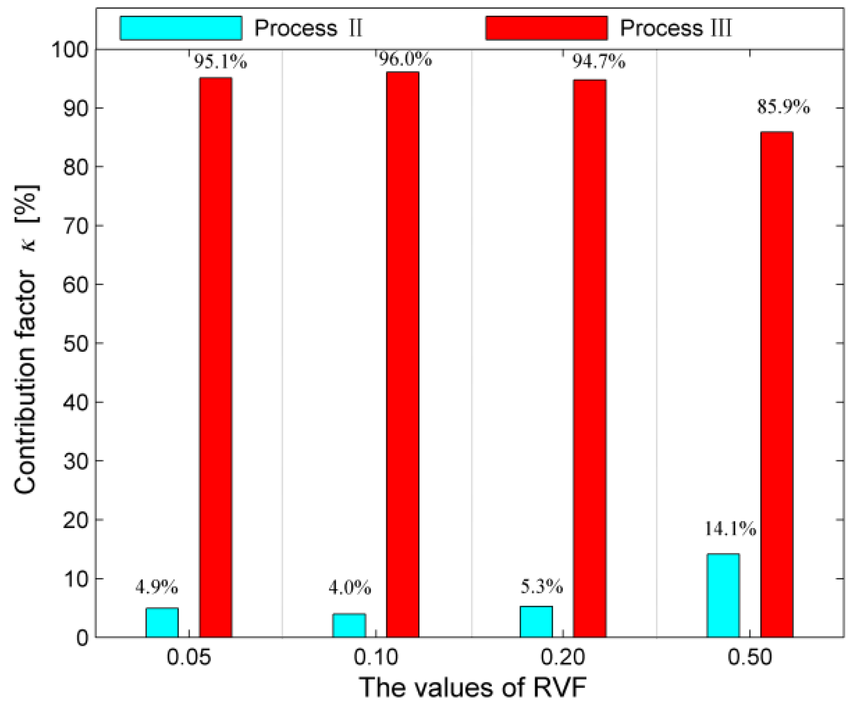
The contribution of Process III to the cutting stability of Process IV is more than 85% and 61% for the associated 1- and 2-DOF systems, respectively. Thus, essentially, VHCVSS is a process in which VHC plays an absolutely leading role for milling stability but VSS plays an auxiliary role.

References

1. Tobias, S.A.; Fishwick, W. Theory of regenerative machine tool chatter. Engineer 1958, 205, 199–203. [Google Scholar]
2. Tlusty, J.; Polacek, M. The stability of machine tools against self-excited vibrations in machining. Int. Res. Prod. Eng. 1963, 115, 1–8. [Google Scholar]
3. Altintas, Y.; Budak, E. Analytical prediction of stability lobes in milling. CIRP Ann. Manuf. Technol. 1995, 44, 357–362. [Google Scholar] [CrossRef]
4. Merdol, S.D.; Altintas, Y. Multi frequency solution of chatter stability for low immersion milling. J. Manuf. Sci. E Trans. ASME 2004, 126, 459–466. [Google Scholar] [CrossRef]
5. Bayly, P.V.; Halley, J.E.; Mann, B.P.; Davies, M.A. Stability of interrupted cutting by temporal finite element analysis. J. Manuf. Sci. E Trans. ASME 2003, 125, 220–225. [Google Scholar] [CrossRef]
6. Butcher, E.A.; Bobrenkov, O.A. On the Chebyshev spectral continuous time approximation for constant and periodic delay differential equations. Commun. Nonlinear Sci. 2011, 16, 1541–1554. [Google Scholar] [CrossRef]
7. Insperger, T.; Stepan, G. Semi-Discretization for Time-Delay Systems Stability and Engineering Applications, 1st ed.; Springer: New York, NY, USA, 2011. [Google Scholar]
8. Insperger, T.; Stepan, G. Semi-discretization method for delayed systems. Int. J. Numer. Methods Eng. 2002, 55, 503–518. [Google Scholar] [CrossRef]
9. Insperger, T.; Stepan, G. Updated semi-discretization method for periodic delay-differential equations with discrete delay. Int. J. Numer. Methods Eng. 2004, 61, 114–141. [Google Scholar] [CrossRef]
10. Olgac, N.; Ergenc, A.; Sipahi, R. Delay scheduling: A new concept for stabilization in multiple delay systems. J. Vib. Control 2005, 11, 1159–1172. [Google Scholar] [CrossRef]
11. Yi, S.; Nelson, P. Delay differential equations via the matrix Lambert W function and bifurcation analysis: Application to machine tool chatter. Math. Biosci. Eng. 2007, 4, 355–368. [Google Scholar]
12. Butcher, E.A.; Bobrenkov, O.A.; Bueler, E.; Nindujarla, P. Analysis of Milling Stability by the Chebyshev Collocation Method: Algorithm and Optimal Stable Immersion Levels. J. Comput. Nonlinear Dyn. 2009, 4, 1–12. [Google Scholar] [CrossRef] [Green Version]
13. He, J.H. Homotopy perturbation technique. Comput. Methods Appl. Mech. Eng. 1999, 178, 257–262. [Google Scholar] [CrossRef]
14. Ding, Y.; Zhu, L.; Zhang, X.; Ding, H. A full-discretization method for prediction of milling stability. Int. J. Mach. Tools Manuf. 2010, 50, 502–509. [Google Scholar] [CrossRef]
15. Liu, Y.; Zhang, D.; Wu, B. An efficient full-discretization method for prediction of milling stability. Int. J. Mach. Tools Manuf. 2012, 63, 40–48. [Google Scholar] [CrossRef]
16. Zatarain, M.; Alvarez, J.; Bediaga, I.; Munoa, J.; Dombovari, Z. Implicit subspace iteration as an efficient method to compute milling stability lobe diagrams. Int. J. Adv. Manuf. Technol. 2015, 77, 597–607. [Google Scholar] [CrossRef]
17. Khasawneh, F.A.; Mann, B.P. Stability of delay integro-differential equations using a spectral element method. Math. Comput. Model. 2011, 54, 2493–2503. [Google Scholar] [CrossRef]
18. Lehotzky, D.; Insperger, T.; Stepan, G. Extension of the spectral element method for stability analysis of time-periodic delay-differential equations with multiple and distributed delays. Commun. Nonlinear Sci. 2017, 35, 177–189. [Google Scholar] [CrossRef] [Green Version]
19. Sosa, J.; Olvera, D.; Urbikain, G.; Martinez-Romero, O.; Elías-Zúñiga, A.; De Lacalle, L.N.L. Uncharted Stable Peninsula for Multivariable Milling Tools by High-Order Homotopy Perturbation Method. Appl. Sci. 2020, 10, 7869. [Google Scholar] [CrossRef]
20. Compeán, F.I.; Olvera, D.; Campa, F.J.; de Lacalle, L.L.; Elías-Zúñiga, A.; Rodríguez, C. Characterization and stability analysis of a multivariable milling tool by the enhanced multistage homotopy perturbation method. Int. J. Mach. Tools Manuf. 2012, 57, 27–33. [Google Scholar] [CrossRef]
21. Urbikain, G.; Lacalle, L.; Campa, F.J.; Fernández, A.; Elías, A. Stability prediction in straight turning of a flexible workpiece by collocation method. Int. J. Mach. Tools Manuf. 2012, 54–55, 73–81. [Google Scholar] [CrossRef]
22. Urbikain, G.; Fernández, A.; Lacalle, L.; Gutiérrez, M. Stability lobes for general turning operations with slender tools in the tangential direction. Int. J. Mach. Tools Manuf. 2013, 67, 35–44. [Google Scholar] [CrossRef]
23. Urbikain, G.; Campa, F.J.; Zulaika, J.J.; De Lacalle, L.N.L.; Alonso, M.A.; Collado, V. Preventing chatter vibrations in heavy-duty turning operations in large horizontal lathes. J. Sound Vib. 2015, 340, 317–330. [Google Scholar] [CrossRef]
24. Urbikain, G.; Olvera, D.; De Lacalle, L.N.L.; Elías-Zúñiga, A. Stability and vibrational behaviour in turning processes with low rotational speeds. Int. J. Adv. Manuf. Technol. 2015, 80, 871–885. [Google Scholar] [CrossRef]
25. Olvera, D.; Urbikain, G.; Elías-Zuñiga, A.; De Lacalle, L.N.L. Improving Stability Prediction in Peripheral Milling of Al7075T6. Appl. Sci. 2018, 8, 1316. [Google Scholar] [CrossRef] [Green Version]
26. Olvera, D.; Elías-Zúñiga, A.; Martínez-Alfaro, H.; de Lacalle, L.L.; Rodríguez, C.; Campa, F. Determination of the stability lobes in milling operations based on homotopy and simulated annealing techniques. Mechatronics 2014, 24, 177–185. [Google Scholar] [CrossRef]
27. Pimenov, D.Y.; Hassui, A.; Wojciechowski, S.; Mia, M.; Magri, A.; Suyama, D.I.; Bustillo, A.; Krolczyk, G.; Gupta, M.K. Effect of the Relative Position of the Face Milling Tool towards the Workpiece on Machined Surface Roughness and Milling Dynamics. Appl. Sci. 2019, 9, 842. [Google Scholar] [CrossRef] [Green Version]
28. Urbikain, G.; Olvera, D.; López de Lacalle, L.N.; Beranoagirre, A.; Elías-Zuñiga, A. Prediction Methods and Experimental Techniques for Chatter Avoidance in Turning Systems: A Review. Appl. Sci. 2019, 9, 4718. [Google Scholar] [CrossRef] [Green Version]
29. Pelayo, G.U.; Olvera-Trejo, D.; Luo, M.; de Lacalle, L.L.; Elías-Zuñiga, A. Surface roughness prediction with new barrel-shape mills considering runout: Modelling and validation. Measurement 2020, 173, 108670. [Google Scholar] [CrossRef]
30. Wan, M.; Zhang, W.-H.; Dang, J.-W.; Yang, Y. A unified stability prediction method for milling process with multiple delays. Int. J. Mach. Tools Manuf. 2010, 50, 29–41. [Google Scholar] [CrossRef]
31. Zhang, X.; Xiong, C.; Ding, Y.; Xiong, Y. Variable-step integration method for milling chatter stability prediction with multiple delays. Sci. China Technol. Sci. 2011, 54, 3137–3154. [Google Scholar] [CrossRef]
32. Jin, G.; Qi, H.; Cai, Y.; Zhang, Q. Stability prediction for milling process with multiple delays using an improved semi-discretization method. Math. Method Appl. Sci. 2016, 39, 949–958. [Google Scholar] [CrossRef]
33. Mei, Y.; Mo, R.; Sun, H.; He, B.; Bu, K. Stability Analysis of Milling Process with Multiple Delays. Appl. Sci. 2020, 10, 3646. [Google Scholar] [CrossRef]
34. Jiang, S.; Sun, Y. Stability analysis for a milling system considering multi-point-contact cross-axis mode coupling and cutter run-out effects. Mech. Syst. Signal Process. 2019, 141, 106452. [Google Scholar] [CrossRef]
35. Sims, N.; Mann, B.; Huyanan, S. Analytical prediction of chatter stability for variable pitch and variable helix milling tools. J. Sound Vib. 2008, 317, 664–686. [Google Scholar] [CrossRef] [Green Version]
36. Sims, N. Fast chatter stability prediction for variable helix milling tools. Proc. Inst. Mech. Eng. Part C J. Mech. Eng. Sci. 2015, 230, 1989–1996. [Google Scholar] [CrossRef] [Green Version]
37. Dombovari, Z.; Stepan, G. The effect of helix angle variation on milling stability. J. Manuf. Sci. E Trans. ASME 2012, 134, 051015. [Google Scholar] [CrossRef]
38. Dombovari, Z.; Altintas, Y.; Stepan, G. The effect of serration on mechanics and stability of milling cutters. Int. J. Mach. Tools Manuf. 2010, 50, 511–520. [Google Scholar] [CrossRef]
39. Jin, G.; Zhang, Q.; Hao, S.; Xie, Q. Stability prediction of milling process with variable pitch and variable helix cutters. Proc. Inst. Mech. Eng. Part C J. Mech. Eng. Sci. 2014, 228, 281–293. [Google Scholar] [CrossRef]
40. Insperger, T.; Stepan, G. Stability analysis of turning with periodic spindle speed modulation via semidiscretization. J. Vib. Control 2004, 10, 1835–1855. [Google Scholar] [CrossRef]
41. Zatarain, M.; Bediaga, I.; Muñoa, J.; Lizarralde, R. Stability of milling processes with continuous spindle speed variation: Analysis in the frequency and time domains, and experimental correlation. CIRP Ann. Manuf. Technol. 2008, 57, 379–384. [Google Scholar] [CrossRef]
42. Long, X.H.; Balachandran, B. Stability of Up-milling and Down-milling Operations with Variable Spindle Speed. J. Vib. Control 2011, 16, 1151–1168. [Google Scholar] [CrossRef]
43. Seguy, S.; Insperger, T.; Arnaud, L.; Dessein, G.; Peigné, G. On the stability of high-speed milling with spindle speed variation. Int. J. Adv. Manuf. Technol. 2010, 48, 883–895. [Google Scholar] [CrossRef] [Green Version]
44. Xie, Q.; Zhang, Q. Stability predictions of milling with variable spindle speed using an improved semi-discretization method. Math. Comput. Simulat. 2012, 85, 78–89. [Google Scholar] [CrossRef]
45. Totis, G.; Albertelli, P.; Sortino, M.; Monno, M. Efficient evaluation of process stability in milling with Spindle Speed Variation by using the Chebyshev Collocation Method. J. Sound Vib. 2014, 333, 646–668. [Google Scholar] [CrossRef]
46. Urbikain, G.; Olvera, D.; de Lacalle, L.L.; Elías-Zúñiga, A. Spindle speed variation technique in turning operations: Modeling and real implementation. J. Sound Vib. 2016, 383, 384–396. [Google Scholar] [CrossRef]
47. Bediaga, I.; Zatarain, M.; Munoa, J.; Lizarralde, R. Application of continuous spindle speed variation for chatter avoidance in roughing milling. Proc. Inst. Mech. Eng. Part B J. Eng. Manuf. 2016, 225, 631–640. [Google Scholar] [CrossRef]
48. Bediaga, I. Regenerative Chatter Suppression by Means of Variable Spindle Speed. Ph.D. Thesis, Department of Mechanical Engineering, Bilbao, Spain, 2009. [Google Scholar]
49. Jin, G.; Qi, H.; Li, Z.; Han, J. Dynamic modelling and stability analysis for the combined milling system with variable pitch cutter and spindle speed variation. Commun. Nonlinear Sci. 2018, 63, 38–56. [Google Scholar] [CrossRef]
50. Jin, G.; Jiang, H.; Han, J.; Li, Z.; Li, H.; Yan, B. Stability analysis of milling process with variable spindle speed and pitch angle considering helix angle and process phase difference. Math. Probl. Eng. 2021, 2021, 1–15. [Google Scholar]
51. Zhang, L.; Hao, B.; Xu, D.; Dong, M. Dynamic milling stability prediction of thin-walled components based on VPC and VSS combined method. J. Braz. Soc. Mech. Sci. Eng. 2020, 42, 1–9. [Google Scholar] [CrossRef]
52. Yang, W.A.; Huang, C. Stability analysis of 2-DOF milling dynamics for simultaneously varying tooth pitch and spindle speed with helix angle effect. Int. J. Adv. Manuf. Technol. 2020, 110, 1163–1177. [Google Scholar] [CrossRef]
53. Powell, K.B. Cutting Performance and Stability of Helical Endmills with Variable Pitch. Doctoral Dissertation, University of Florida, Gainesville, FL, USA, 2008. [Google Scholar]
54. Altintas, Y.; Engin, S.; Budak, E. Analytical stability prediction and design of variable pitch cutters. J. Manuf. Sci. E Trans. ASME 1999, 121, 173–179. [Google Scholar] [CrossRef]
Figure 1. Schematic drawing of the process combinations associated with VSS and VPC/VHC. (a) constant speed; (b) VSS; (c) conventional cutter; (d) VPC; (e) VHC
Applsci 11 04203 g001
Figure 2. Schematic mechanical model of the milling system [7]. (a) 1-DOF; (b) 2-DOF; (c) regeneration effect.
Applsci 11 04203 g002
Figure 3. Schematic drawing of the relationship of the segmentation of the axial depth of cut and time delay.
Applsci 11 04203 g003
Figure 4. Comparisons of the SLDs associated with Processes I, II, III, and IV for the 1-DOF system. Note that the SLDs for Processes II and IV are plotted under the conditions of different RVF: (a) RVF = 0.05; (b) RVF = 0.1; (c) RVF = 0.2; and (d) RVF = 0.5.
Applsci 11 04203 g004
Figure 5. Comparisons of the values of χ associated with SLDs in Figure 4.
Applsci 11 04203 g005
Figure 6. Contribution factor diagram of Processes II and III to the combination effect under different RVF.
Applsci 11 04203 g006
Figure 7. Comparison of the SLDs by theoretical prediction and time-domain simulation for different processes. (a) Process I; (b) Process II; (c) Process III; (d) Process IV.
Applsci 11 04203 g007
Figure 8. Comparisons of the SLDs associated with Processes I, II, III, and IV for the 2-DOF system. Note that the SLDs for Processes III and IV are plotted under the conditions of the same pitch angles ( ψ = [70, 110, 70, 110]°) but different helix angles: (a) β = [30, 30, 30, 30]°; (b) β = [32, 30, 32, 30]°; (c) β = [34, 30, 34, 30]°; and (d) β = [36, 30, 36, 30]°.
Applsci 11 04203 g008
Figure 9. Comparison of the values of χ corresponding to the SLDs in Figure 8.
Applsci 11 04203 g009
Figure 10. Contribution factor diagram of Processes II and III to the combination effect under different β .
Applsci 11 04203 g010
Publisher’s Note: MDPI stays neutral with regard to jurisdictional claims in published maps and institutional affiliations.