Method of Estimation of Turbulence Integral Parameters

Abstract

The optical effects of turbulence are directly related to turbulence integral parameters, which are integrals of the refractive index structure constant over a whole path with different path-weighting functions (PWFs). We describe a method that utilizes measurable turbulence integral parameters, such as angle-of-arrival fluctuations and scintillation, to estimate turbulence integral parameters that cannot be measured directly. The estimates of the turbulence integral parameters are based on the linear combination of the PWFs of those measurable quantities. New measurable quantities and their PWFs under different propagation conditions were studied. Some interesting and meaningful results have been obtained. This method shows the prospect of characterizing anisoplanatism in adaptive optics and allows for the estimation of some optical turbulence parameters under non-ideal conditions, such as an isoplanatic angle in a finite distance.

1. Introduction

A wave propagating through a turbulent atmosphere is subject to perturbations of its phase and amplitude due to the fluctuations of the refractive index along the whole propagation path. These perturbations, known as wavefront distortions, severely influence the performance of optical systems that operate in or through the atmosphere, such as adaptive optics systems, interferometers, optical wireless communication systems, and laser radar systems [1,2,3]. Therefore, it is important to understand how the effects of atmospheric turbulence on the propagation of a light wave can be quantified.

Clearly, the turbulence strength at each position of the propagation path contributes to the wavefront distortion. Therefore, the optical turbulence parameters that describe the optical effects of turbulence are often related to turbulence integral parameters, i.e., integrals of the refractive index structure constant Cn²(z) (z denotes the position along the propagation path with the receiver plane at z = 0) over a whole path with different path-weighting functions (PWFs). For example, the atmospheric coherence length for plane waves r_0,p has a PWF of z⁰, the atmospheric coherence length for spherical waves r_0,s has a PWF of (L-z)^5/3, and the isoplanatic angle θ₀ has a PWF of z^5/3 [3]. In a practical situation, these optical turbulence parameters are often measured indirectly using only one measurable turbulence integral parameter, such as in the case of the differential image motion monitor (DIMM) [4], where angle-of-arrival fluctuations are measured, and in the case of the stellar scintillation isoplanometer [5,6], where intensity fluctuations (scintillation) are measured. However, in many applications, some of the desired optical turbulence parameters cannot be estimated using only one measurable quantity, especially due to the anisoplanatic problems in adaptive optics [7,8], where the expression of related PWFs is more complex and can only be evaluated numerically. For example, in the angular or focal anisoplanatic problems in adaptive optics, the PWF of the effective phase variance (the total phase variance with the piston removed or both the piston and the tilt removed) is neither z⁰ nor z^5/3, so it cannot be estimated properly by r₀ or θ₀ [7,8,9].

In this paper, we relate the optical effects of turbulence to the path-weighting functions (PWFs) and describe a method (referred to as the linear combination method) that uses more than one measurable turbulence integral quantity to estimate the turbulence integral parameters that cannot be measured directly. We generalize the PWFs of measurable integral parameters and investigate their characteristics in both a plane wave model and a spherical wave model for the common case where one source is used and the receive apertures are unobscured circles. Some interesting and meaningful results have been obtained. These results may enable us to measure r₀ not only at near-field but also at far-field using the covariance of tilt, and to measure θ_TA using a small-aperture telescope instead of a large-aperture telescope using the covariance of intensity rather than scintillation.

2. Materials and Methods

The turbulence integral parameter noted as P is written as follows:

$$P=CL{\displaystyle {\int }_0^1{C}_n^2(uL)}W(u)du$$

(1)

where C is a constant related to P, L is the propagation path length through turbulence, C_n² is the turbulence strength, W(u) is the PWF, and u = z/L denotes the normalized position along the path with propagation from u = 1 to u = 0 at the receiver. The principle of the linear combination method is that any linear combination of turbulence integral parameters corresponds to the linear combination of their PWFs. The desired integral parameter P_d can be estimated from measurable integral parameters P_i if only the PWF of P_d, noted as W_d(u), can be approximated by linear combination of the PWFs of P_i, noted as W_i(u), i.e.,

$$W_d(u)\approx {\displaystyle \sum _{i=1}^N{a}_i{W}_i(u)}$$

(2)

where a_i are the coefficients of W_i(u), and N is the number of measurable integral parameters used in this method. In practical applications, one should first select a suitable W_i(u) based on the shape of W_d(u) and then fit W_i(u) to W_d(u) using the least square fitting method. Equation (2) shows that the more measurable integral parameters and their PWFs we know, the more desired PWFs we can approximate using this method and, thus, the more integral parameters we can estimate. Therefore, it is important to investigate more measurable quantities and their PWFs.

Atmospheric turbulence causes phase and amplitude perturbations, and at present, only the tilt phase and piston amplitude, corresponding to the angle of arrival and the intensity of the light collected with an aperture, can be measured directly and relatively easily. In practice, the variance of the angle of arrival and the variance of intensity are used to obtain turbulence information through their PWFs, which is exactly the case in the DIMM and the stellar scintillation isoplanometer, respectively. However, the covariance functions for the angle of arrival or intensity provide more turbulence information due to their potentially large number of PWFs. The covariance of the tilt phase can be measured from the covariance of the angle of arrival [3,4], and the covariance of the piston amplitude can be measured from the covariance of intensity [6,10].

Assuming the Rytov approximation and Kolmogorov turbulence, using the analytic approach developed by Sasiela [3], the covariance functions for the phase and the log-amplitude related quantities can be derived as follows:

$$\left[\begin{array}{l}{C}_{\varphi }(d)\\ C_{\chi }(d)\end{array}\right]=0.132{\pi }^2{k}^{2}L{\displaystyle {\int }_0^1{C}_n^2(uL)}\left[\begin{array}{l}{W}_{C,\varphi }(u)\\ W_{C,\chi }(u)\end{array}\right]du$$

(3)

where φ and α denote the phase and the log-amplitude related quantities, respectively; d is the center-to-center distance of two receive apertures; the optical wavenumber k = 2π/λ, where λ is the wavelength of the observed beacon; and W_C,φ(u) and W_C,χ(u) are path-weighting functions which are given by the following:

$$\left[\begin{array}{l}{W}_{C,\varphi }(u)\\ W_{C,\chi }(u)\end{array}\right]={\displaystyle {\int }_0^{\infty }\kappa F(\gamma \kappa )J_0(\gamma \kappa d){\kappa }^{-11/3}\left[\begin{array}{l}{\cos }^2(\frac{{\kappa }^2\gamma uL}{2k})\\ {\sin }^2(\frac{{\kappa }^2\gamma uL}{2k})\end{array}\right]}d\kappa$$

(4)

where κ is the spatial wavenumber transverse to the z direction; γ is the propagation parameter, which depends on the geometric divergence of the light wave and has the simple value of γ = 1 for plane waves and γ = 1−z/L for spherical waves; J_n is the nth order Bessel function of the first kind; and F(γκ) is the filter function, which depends on propagation geometry, such as the size of the receive aperture and the distributed source, and measured related quantities, such as the tilt phase or piston amplitude. For circular apertures with diameter D, the filter function for Zernike tilt and piston are as follows [3]:

$$F_t(\gamma \kappa )={\left[8J_2(\gamma \kappa D/2)/\gamma \kappa D\right]}^2 (\mathrm{Tilt})$$

(5)

$$F_p(\gamma \kappa )={\left[4J_1(\gamma \kappa D/2)/\gamma \kappa D\right]}^2 (\mathrm{Piston})$$

(6)

For a uniformly illuminated circular source with diameter D_s located at a distance L_S, considering that the uniform circular source consists of incoherent point beacons, the source filter function is as follows [3]:

$$F_s(\gamma \kappa )={\left[4L_s{J}_1(\kappa D_{s}z/2L_s)/\kappa D_{s}z\right]}^2$$

(7)

The final filter function is the product of any produced filter functions. Make a change to the variables by replacing κD with x and use the replacement F_N = D²/λL, where F_N is the Fresnel number, to simplify the final expression of the PWFs for the tilt phase (i.e., substituting F(γκ) = F_t(γκ) * F_s(γκ) into Equation (4)) and piston amplitude (i.e., substituting F(γκ) = F_p(γκ) * F_s(γκ) into Equation (4)), noted as W_C,T(u), W_C,P(u), to the following:

$$\left[\begin{array}{l}{W}_{C,T}(u)\\ W_{C,P}(u)\end{array}\right]=D^{\frac{5}{3}}{\displaystyle {\int }_0^{\infty }\left[\begin{array}{l}{\left[8J_2(\gamma x/2)/\gamma x\right]}^2\\ {\left[4J_1(\gamma x/2)/\gamma x\right]}^2\end{array}\right]{\left[2\frac{J_1(\frac{xu{D}_{s}L}{2D{L}_s})}{\frac{xu{D}_{s}L}{2D{L}_s}}\right]}^2{J}_0(\gamma x\frac{d}{D})x^{-\frac{8}{3}}\left[\begin{array}{l}{\cos }^2(\frac{x^2\gamma u}{4\pi F_N})\\ {\sin }^2(\frac{x^2\gamma u}{4\pi F_N})\end{array}\right]}dx$$

(8)

From Equation (8), it is clear that the PWFs for the tilt phase and piston amplitude depend on four variables: γ, d/D, F_N, and D_SL/DL_S (i.e., the ratio of the angular diameter of the source to that of the receive aperture observed at plane z = L). In the following sections D_SL/DL_S will be noted as R for simplicity. Any change in these four variables will result in a new PWF. 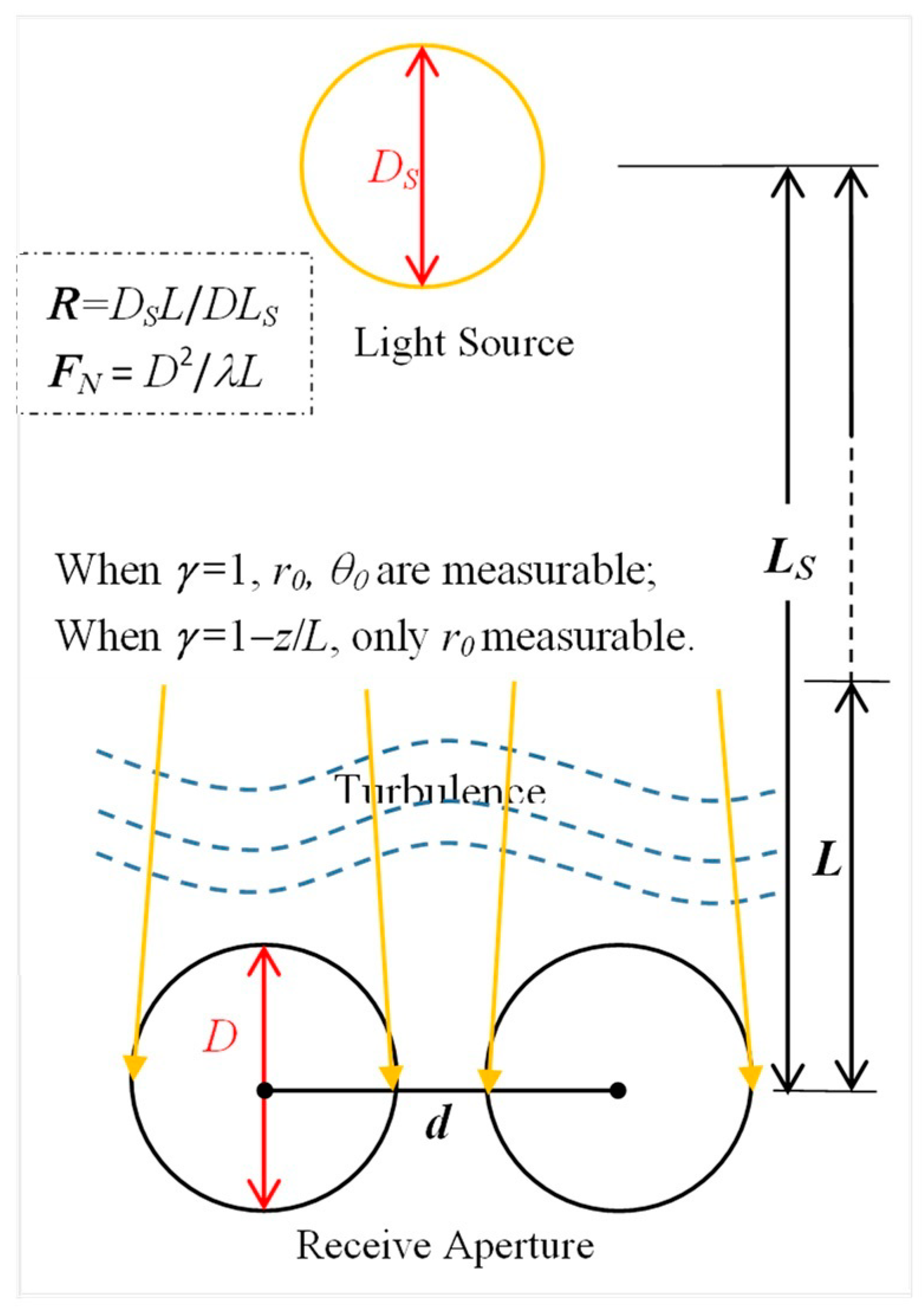Obviously, we can obtain more PWFs by using the covariance function instead of the variance function, which is the special case of the covariance function for d = 0. The geometry and variables of the covariance functions are shown in Figure 1 for reference.

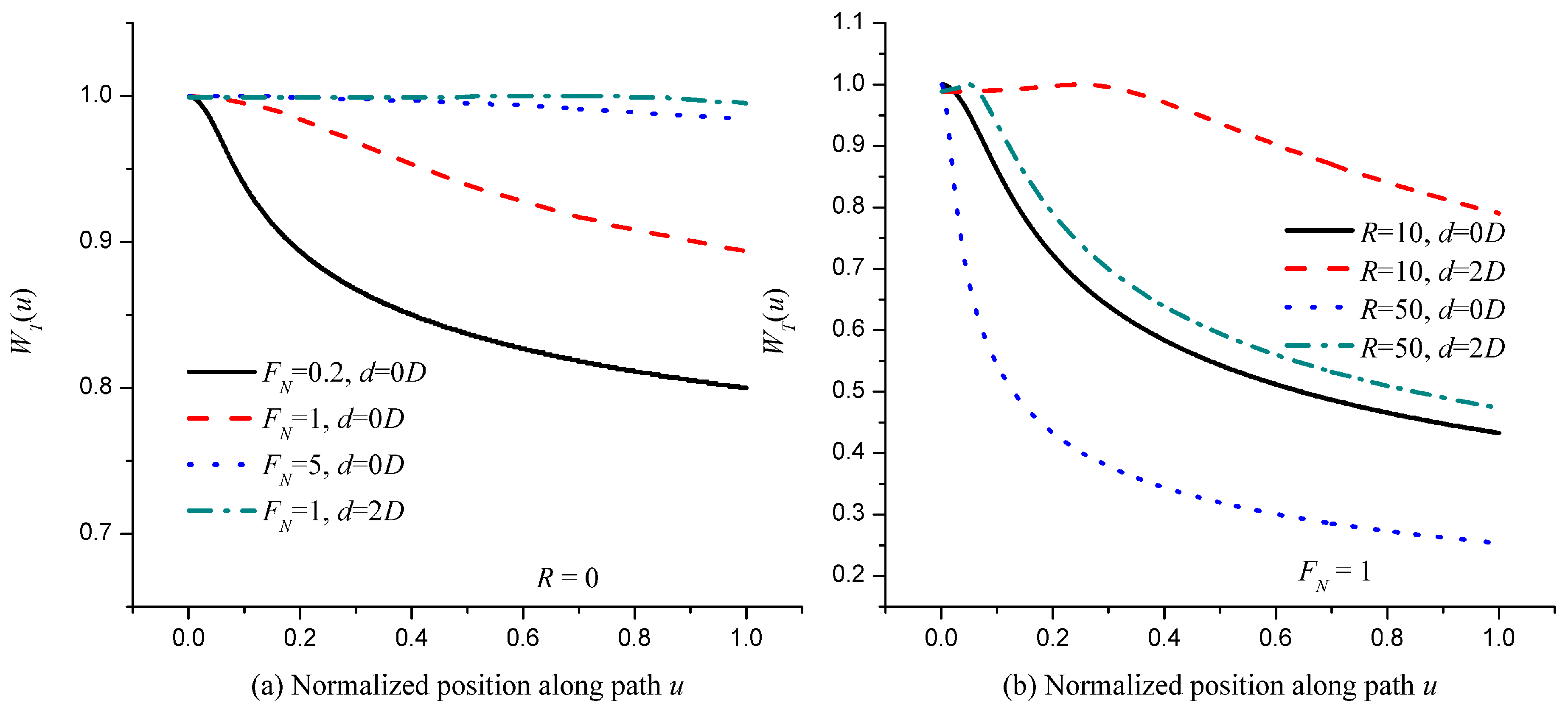
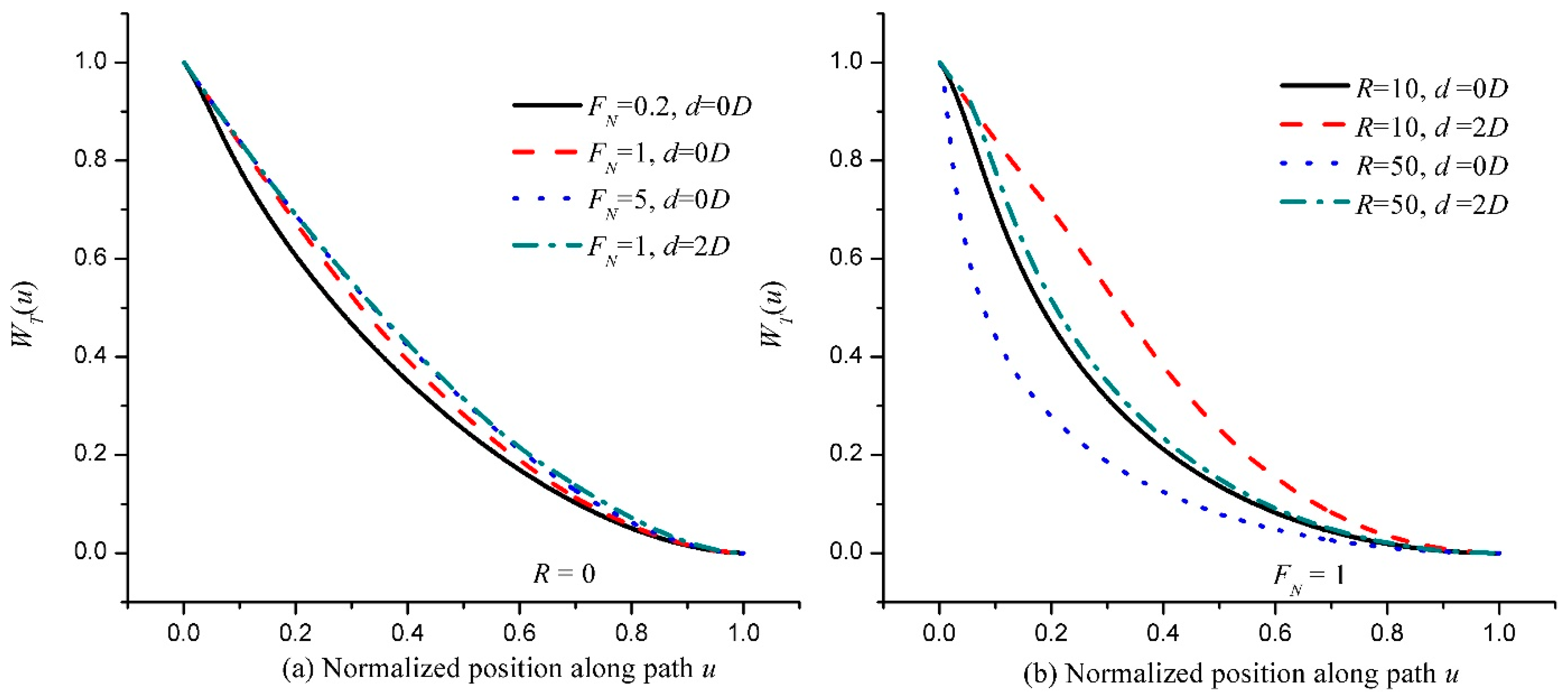
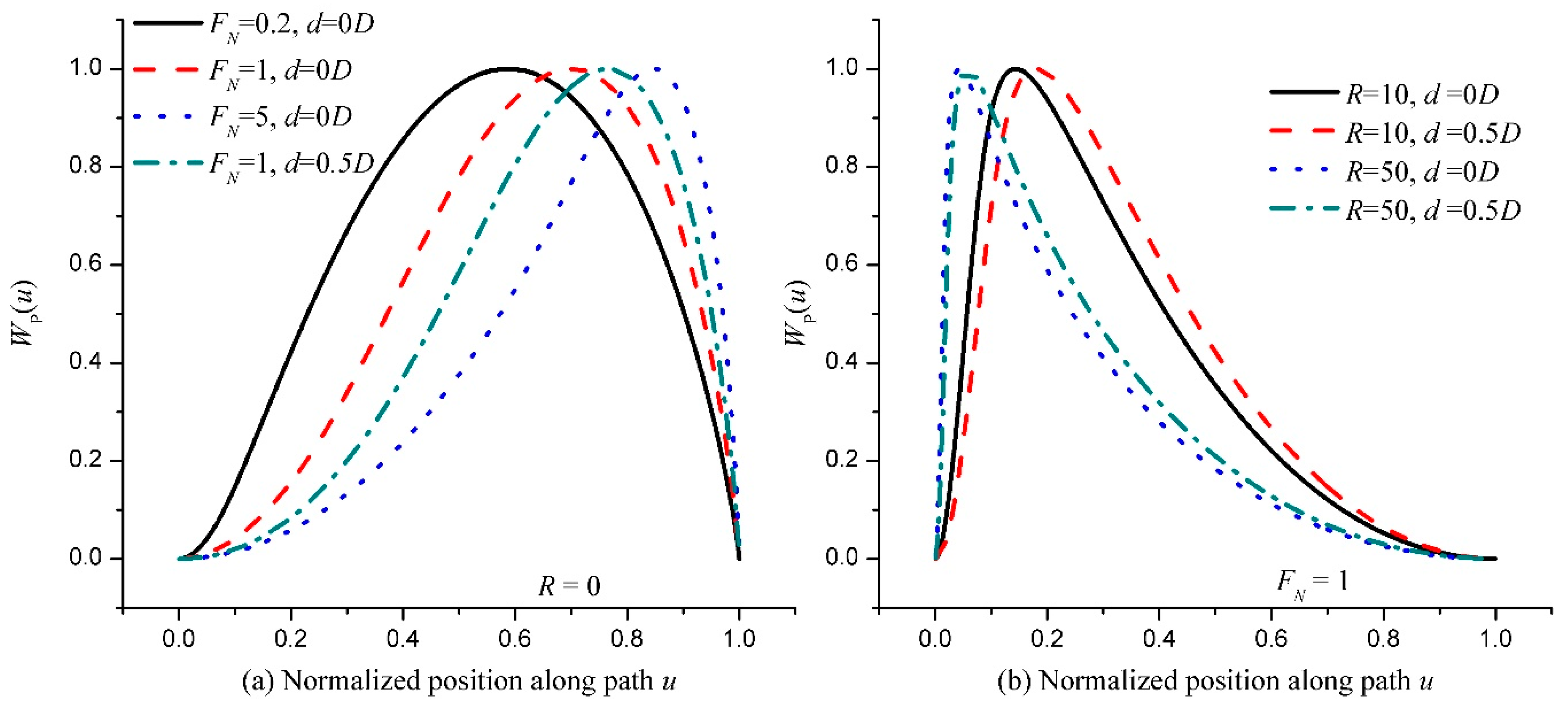
For convenience later, denote W_T(u) as the normalized PWF for the covariance of the tilt phase, and W_P(u) as the normalized PWF for the covariance of piston amplitude. To obtain qualitative knowledge of the effects of these four variables on the PWFs, next we will give the PWFs in a range of typical conditions by numerical evaluation.

3. Results

3.1. PWFs for Plane Waves

Consider Plane Waves (L_S Well above the Turbulent Atmosphere) for Which γ = 1. W_T(u) for Different d, F_N, and R is Plotted in Figure 2.

For a point source such as a star, for which R = 0, the W_T(u) for different F_N and d values is shown in Figure 2a. It can be seen that F_N influences the PWF of the tilt phase variance (W_T(u) for d = 0) as expected. Due to the effect of diffraction [3,4], the W_T(u) for d = 0 decreases slowly with u, which deviates from the near-field value that is constant along the path, and the deviation becomes notable when F_N < 1, suggesting that the smaller the F_N is, the bigger the deviation is. This explains why the DIMM operates at the near-field approximation (big F_N). Comparing W_T(u) for F_N = 1, d = 0D (dash line) and F_N = 1, d = 2D (dash dot line) shows that the effect of diffraction on the tilt covariance is far smaller than that on the tilt variance, which indicates that the effect of diffraction appears to be partly counteracted by the covariance term J₀(γκ d/D) (see Equation (8)). For a distributed source such as a planet, the W_T(u) for different R and d values with a fixed Fresnel number F_N = 1 is shown in Figure 2b. It can be seen that the W_T(u) for d = 0 decreases significantly with u. For larger R values, the downward trend of W_T(u) is more obvious (dot line versus solid line). By comparing the W_T(u) for d = 0 and d = 2D with the same R value, again we can see that the effect of diffraction on the tilt covariance is smaller than that on the tilt variance.

For plane waves, the W_P(u) values for different d, F_N, and R values are plotted in Figure 3.

For a point source such as a star, for which R = 0, the W_P(u) for different F_N and d values is shown in Figure 3a. It can be seen immediately that the asymptotic behavior of the W_P(u) for d = 0 with respect to F_N is consistent with well-known asymptotic behavior [5], i.e., the PWFs of stellar scintillations (W_P(u) for d = 0) are approximate to u^5/6 for a small D (i.e., small F_N when λL is fixed) and u² for a large D. When the selected F_N is satisfactory (approximately equals one, dash line), the W_P(u) for d = 0 is approximate to u^5/3, which is needed to calculate the isoplanatic angle [5,6]. In Figure 3a, there is a remarkable place where the curves of W_P(u) for d = 0.5D, F_N = 1 and d = 0D, F_N = 5 seem almost identical, both approximating u², which is needed to calculate the tilt isoplanatic angle (θ_TA) [1,3]. For a distributed source such as the sun or a planet, the W_P(u) for different R and d values with a fixed Fresnel number F_N = 1 is shown in Figure 3b. It can be seen that the peak position of W_P(u) with the same d value moves toward the start of the path with the increase in the R value, and that the peak position of W_P(u) with the same R value shifts slightly toward the end of the path with the increase in the d value. When the receiver size D is very small and the distributed source is the sun or the moon, we will obtain the PWFs that are used in SHABAR [11] (SHAdow BAnd and Ranging) or LuSci [12] (Lunar Scintillometer), both of which are used to measure surface layer turbulence.

3.2. PWFs for Spherical Waves

Now Consider Spherical Waves (i.e., L_S equal to L) for Which γ = 1−u. W_T(u) for Different d, F_N, and R is Plotted in Figure 4.

For a point source, the W_T(u) for different F_N and d values is shown in Figure 4a. Not surprisingly, for d = 0, the W_T(u) for a large F_N value (dot line) has the form (1−u)^5/3 that can be used to measure r_0,s; the W_T(u) for a small F_N value deviates slightly from (1−u)^5/3 due to the effect of diffraction. The two curves of W_T(u) for d = 0D, F_N = 5 and d = 2D, F_N = 1 almost coincide with each other, as the effect of diffraction on the tilt covariance is smaller than that on the variance. For a distributed source, the W_T(u) for different R and d values and a fixed Fresnel number F_N = 1 is shown in Figure 4b. It can be seen that the W_T(u) for a finite-size source deviates significantly from (1−u)^5/3; therefore, the larger the R value is, the faster the decline in W_T(u) is. When comparing the W_T(u) for d = 0 and d = 2D, again we can see that the effect of diffraction on the tilt covariance is smaller than that on the tilt variance.

For spherical waves, W_P(u) for different d, F_N and R values are plotted in Figure 5.

One can see that the peak position of W_P(u) for fixed d and R values moves towards the end of the path with an increasing F_N value, as shown in Figure 5a; that the peak position of W_P(u) for fixed F_N and d values moves towards the start of the path with an increasing R value, as shown in Figure 5b; and that the peak position of W_P(u) for fixed F_N and R values moves towards the end of the path with an increasing d value, as shown in Figure 5a,b.

4. Discussion

From the above numerical results, we can see how each of the four variables (γ, d/D, F_N, and R) influence the curve shapes of PWFs, which is helpful in the creation of a desired PWF using the linear combination method (Equation (2)). When we focused on the PWFs for different F_N values without changing the other variables, we found that the effect of diffraction on the covariance of the tilt phase or piston amplitude is far smaller than that on the variance.

Note that the PWFs investigated here only considered the common case where one source is used and the receive apertures are unobscured circles. When the shape of the receive aperture is changed or two sources are used, the curve shapes of the related PWFs will also change, as in the case of MASS [13] (Multi-Aperture Scintillation Sensor), where the receive aperture is annulus, or SloDAR [14] (Slope Detection And Ranging) and SciDAR [15,16] (Scintillation Detection And Ranging), where two sources are used. Thus, there are potentially a large number of various W_i(u) values that we can obtain, which would make the linear combination method more powerful.

In some applications, the PWFs of P_d (the desired turbulence integral parameter) have complex analytic expressions, most of which can only be evaluated numerically, and P_d is often difficult to measure at present. For example, in the angular or focal anisoplanatic problems in adaptive optics, the effective phase variance σ²_Eff (the total phase variance σ²_φ with the piston removed or both the piston σ²_P and the tilt σ²_TA removed, i.e., σ²_Eff = σ²_φ−σ²_P (−σ²_TA)) is such a P_d [3,7,8,9]. For natural guide star adaptive optics (NGS AO), it is well known that σ²_φ = (θ/θ₀)^5/3, and one can easily derive σ²_P = 4.25 σ²_TA = 4.25 (θ/θ_TA)² for small angles, where θ_TA is the tilt isoplanatic angle [1,3,17]. Therefore, if θ_TA can be measured along with θ₀, one can obtain the effective phase variance in NGS AO using the relationship σ²_Eff = (θ/θ₀)^5/3 − 4.25(θ/θ_TA)² (−(θ/θ_TA)²). As far as we know, the direct measurement of θ_TA has not been reported. Based on the linear combination method proposed in this paper, we have proposed one direct measurement scheme of θ_TA in our other accompanying manuscript [18].

In some other applications, though expressions for the PWF of P_d are simple, it cannot be measured under non-ideal conditions. For example, r_0,p and θ₀ in a finite distance cannot be measured using the conventional method (DIMM and stellar scintillation isoplanometer) since the light wave propagating in the turbulence path is not a plane wave. Generally, the light wave is a spherical wave for a point beacon in a finite distance. Then, the parameter measured using DIMM is actually r_0,s rather than r_0,p, and the parameter measured using the conventional isoplanometer has a PWF with a curve shape similar to the red dashed line in Figure 5a rather than the red dashed line in Figure 3a (i.e., the well-known u^5/3).

The linear combination method shows promise of estimating the real-time P_d with high accuracy if the suitable W_i(u) can be found. As an application example of this method, one can measure the isoplanatic angle in a finite distance through the combination of one spherical wave scintillation and two covariances of intensity in three receive apertures [10], and the validity of this method was proven by real data from the validation experiment [19].

One can also roughly estimate P_d through the optical turbulence profile obtained from those turbulence profilers [12,13,14,15,16]. Nevertheless, the linear combination method offers another feasible solution.

5. Conclusions

It was found that the path-weighting functions (PWFs) for covariance depend on four variables: γ, d/D, F_N, and D_SL/DL_S. In other words, the optical effects of turbulence are influenced by not only the turbulence strength but also these four variables. Numerical results show that the effect of diffraction on the variance of the tilt phase or piston amplitude ismore significant than it is on the covariance, e.g., the two curves of W_T(u) for d = 0D, F_N = 5 and d = 2D, F_N = 1 almost coincide with each other, and it is possible to measure the tilt isoplanatic angle through the covariance of intensity rather than scintillation. More specifically, the curve of the PWFs for the tilt phase shifts upwards as the value of d/D or F_N increases, or the value of R (R = D_SL/DL_S) decreases (see Figure 2 and Figure 4). The peak position of W_P(u) shifts to the start of the path as the value of d/D or F_N decreases, or the value of R increases (see Figure 3 and Figure 5).

In the future, work will be conducted to prove the validity of measuring the tilt isoplanatic angle through the covariance of intensity and to investigate more suitable PWFs for practical applications. The linear combination method is an effective and powerful method for measuring the turbulence integral parameters of interest as there are a potentially large number of various PWFs that we can obtain.

References

1. John, W.H. Adaptive Optics for Astronomical Telescopes; Oxford University Press: Oxford, UK, 1998. [Google Scholar]
2. Andrews, L.C.; Phillips, R.L. Laser Beam Propagation through Random Media; SPIE: Bellingham, WA, USA, 2005. [Google Scholar]
3. Sasiela, R.J. Electromagnetic Wave Propagation in Turbulence: Evaluation and Application of Mellin Transforms, 2nd ed.; SPIE: Bellingham, WA, USA, 2007. [Google Scholar]
4. Sarazin, M.; Roddier, F. The ESO differential image motion monitor. Astron. Astrophys. 1990, 227, 294–300. [Google Scholar]
5. Loos, G.C.; Hogge, C.B. Turbulence of the upper atmosphere and isoplanatism. Appl. Opt. 1979, 18, 2654–2661. [Google Scholar] [CrossRef] [PubMed]
6. Longkun, Y.; Hong, S.; Xu, J.; Zaihong, H.; Yi, W. Study on the Measurement of θ0 using stellar scintillation. Acta Opt. Sin. 2014, 34, 0301001. [Google Scholar] [CrossRef]
7. Stone, J.; Hu, P.H.; Mills, S.P.; Ma, S. Anisoplanatic effects in finite-aperture optical systems. J. Opt. Soc. Am. A 1994, 11, 347–357. [Google Scholar] [CrossRef]
8. Phillip, D.S. Anisoplantism in Adaptive Optics Compensation of a Focused Beam Using Distributed Beacons. J. Opt. Soc. Am. A 1996, 13, 868–874. [Google Scholar]
9. van Dam, M.A.; Sasiela, R.J.; Bouchez, A.H.; Le Mignant, D.; Campbell, R.D.; Chin, J.C.; Hartman, S.K.; Johansson, E.M.; Lafon, R.E.; Stomski, P.J., Jr.; et al. Angular Anisoplanatism in Laser Guide Star Adaptive Optics; SPIE: Bellingham, WA, USA, 2006; p. 6272. [Google Scholar]
10. Yu, L.K.; Jing, X.; Shen, H.; Hou, Z.H.; Wu, Y. Isoplanatic angle in finite distance: Theory analysis on measurement feasibility. Opt. Lett. 2014, 39, 789–792. [Google Scholar] [CrossRef] [PubMed]
11. Beckers, J.M. Seeing Monitor for Solar and other Extended Object Observations. Exp. Astron. 2001, 12, 1–20. [Google Scholar] [CrossRef]
12. Tokovinin, A.; Bustos, E.; Berdja, A. Near-ground turbulence profiles from lunar scintillometer. Mon. Not. R. Astron. Soc. 2010, 404, 1186–1196. [Google Scholar] [CrossRef] [Green Version]
13. Tokovinin, A.; Kornilov, V.; Shatsky, N.; Voziakova, O. Restoration of turbulence profile from scintillation indices. MN-RAS 2003, 343, 891–899. [Google Scholar] [CrossRef] [Green Version]
14. Wilson, R.W. SLODAR: Measuring optical turbulence altitude with a Shack–Hartmann wavefront sensor. MN-RAS 2002, 337, 103–108. [Google Scholar] [CrossRef] [Green Version]
15. Avila, R.; Vernin, J.; Sanchez, L.J. Atmospheric turbulence and wind profile monitoring with generalized scidar. Astron. Astrophys. 2001, 369, 364–372. [Google Scholar] [CrossRef]
16. Shepherd, H.W.; Osborn, J.; Wilson, R.W.; Butterley, T.; Avila, R.; Dhillon, V.S.; Morris, T.J. Stereo-SCIDAR: Optical turbulence profiling with high sensitivity using a modified SCIDAR instrument. MN-RAS 2014, 437, 3568–3577. [Google Scholar] [CrossRef]
17. Chen, J.; Chang, X. A Unified Approach to Analysing the Anisoplanatism of Adaptive Optical Systems. In Adaptive Optics Progress; Tyson, R.K., Ed.; IntechOpen: Rijeka, Croatia, 2012. [Google Scholar]
18. Shen, H.; Yu, L.K.; Jing, X.; Tan, F. Method for Measuring the Second-order Moment of Atmospheric Turbulence. Atmosphere 2021, 12, 564. [Google Scholar] [CrossRef]
19. Yu, L.K.; Hou, Z.; Zhang, S.C.; Jing, X.; Wu, Y. Isoplanatic angle in finite distance: Experimental validation. Opt. Eng. 2015, 54, 024105. [Google Scholar] [CrossRef]
Figure 1. The geometry and variables for the covariance functions.
Applsci 11 04157 g001
Figure 2. Normalized path-weighting function WT(u) for plane waves. (a) Point sources with various FN (FN = D2/λL) and d (the distance between the aperture centers) values. (b) Distributed sources with various R (R = DSL/DLS) and d values when FN = 1.
Applsci 11 04157 g002
Figure 3. Normalized path-weighting function WP(u) for the covariance of piston amplitude for plane waves. (a) Point sources with various FN (FN = D2/λL) and d (the distance between the aperture centers) values. (b) Distributed sources with various R (R =DSL/DLS) and d values when FN = 1.
Applsci 11 04157 g003
Figure 4. Normalized path-weighting function WT(u) for spherical waves. (a) Point sources with various FN (FN = D2/λL) and d (the distance between aperture centers) values. (b) Distributed sources with various R (R = DSL/DLS) and d values when FN = 1.
Applsci 11 04157 g004
Figure 5. Normalized path-weighting function for the covariance of piston amplitude WP(u) for spherical waves. (a) Point sources with various FN (FN = D2/λL) and d (the distance between aperture centers) values. (b) Distributed sources with various R (R = DSL/DLS) and d values when FN = 1.
Applsci 11 04157 g005
Publisher’s Note: MDPI stays neutral with regard to jurisdictional claims in published maps and institutional affiliations.