Health Indicators Construction and Remaining Useful Life Estimation for Concrete Structures Using Deep Neural Networks

Abstract

Remaining useful life (RUL) prognosis is one of the most important techniques in concrete structure health management. This technique evaluates the concrete structure strength through determining the advent of failure, which is very helpful to reduce maintenance costs and extend structure life. Degradation information with the capability of reflecting structure health can be considered as a principal factor to achieve better prognosis performance. In traditional data-driven RUL prognosis, there are drawbacks in which features are manually extracted and threshold is defined to mark the specimen’s breakdown. To overcome these limitations, this paper presents an innovative SAE-DNN structure capable of automatic health indicator (HI) construction from raw signals. HI curves constructed by SAE-DNN have much better fitness metrics than HI curves constructed from statistical parameters such as RMS, Kurtosis, Sknewness, etc. In the next stage, HI curves constructed from training degradation data are then used to train a long short-term memory recurrent neural network (LSTM-RNN). The LSTM-RNN is utilized as a RUL predictor since its special gates allow it to learn long-term dependencies even when the training data is limited. Model construction, verification, and comparison are performed on experimental reinforced concrete (RC) beam data. Experimental results indicates that LSTM-RNN generally estimates more accurate RULs of concrete beams than GRU-RNN and simple RNN with the average prediction error cycles was less than half compared to those of the simple RNN.

1. Introduction

The last decades have witnessed the explosive increase in the construction industry to meet the unceasing demand for civilian, industrial, and defense purposes. Regardless of the purpose, one of the most significant criteria for structural materials is durability. Even though concrete is one of the most popular materials for construction, brittleness can make it vulnerable to deterioration through cracking progression. The cracking phenomenon is crucial to structure safety and economics, and it has therefore been frequently studied [1,2,3,4]. Besides fault diagnosis and classification (FDC) algorithms that have been widely used to detect and isolate incipient faults in many applications [5,6,7]. Fault prognosis methods have been increasingly receiving more attention in the recent time [8,9]. With prognosis, imminent failures can be reported, and maintenance can be performed accordingly.

An essential metric for prognostic methods is the remaining useful life (RUL), which is also called lead time or prognostic distance. It is defined as the duration from the current time when a specimen is being inspected until its expected useful life expires [9,10]. The prediction of RUL can be performed by two main approaches: data-driven and model-based. Model-based methods represent damage progression by analytical models [11], wherein the researchers need to capture the nature of both the failure and the system. In contrast, estimating RUL with available data in data-driven methods does not need the exact failure mechanisms for data-driven modeling. Therefore, they have been in favor in recent studies [12].

The data-driven approach to prognosis can be divided into three stages: data acquisition, construction of health indicators (HIs), and then prognostics. To monitor and highlight the fracture occurrences, acoustic emission (AE) is commonly used for data acquisition, being able to detect both external and internal damage on the structure [13,14,15]. Therefore, AE is utilized here to study the deterioration of a concrete structure during a loading process until its final failure. The second stage, which constructs HIs, can strongly affect the accuracy of the RUL [9]. Most data-driven methods form HIs from statistical parameters, among which kurtosis and root mean square (RMS) are used most often. Williams et al. [16] proposed the direct use of these two parameters for bearing vibration signal quantification, while Antoni [17] suggested spectral kurtosis in bearing health monitoring, which is considered one of the most intriguing and effective HI construction methods. In this approach, the kurtosis can be calculated by the fourth-order central moment over the squared second-order central moment. In addition to these two parameters, the smoothness index [18] is also important. This parameter is the result of the geometric mean over the arithmetic mean of the modulus of the wavelet coefficients.

In recent years, synthesized HIs have attracted increasing attention [19]. They are often formed by data fusion techniques that combine multi-dimensional features such as RMS, kurtosis, and variance into one-dimensional HIs [9,10,20]. Even though synthesized HIs have achieved spectacular performance and results, there are still disadvantages to be overcome. The first major problem is the uneven contribution of inputs to HI construction, which is the consequence of different features having different ranges. The second major problem is the difficulty in determining the failure threshold, which depends on the specific specimen at hand.

Deep learning techniques have recently been successfully applied in many areas, including natural language processing, computer vision, and robotics [21,22]. They have displayed a promising competence to extract features automatically during the requisite training period. End-to-end classification models with direct mapping to the output classes from raw input can be constructed without manual feature extraction to establish an intermediate feature space. In order to solve the problems of uneven inputs and difficulty in determining the failure threshold described earlier, this paper proposes the development of a deep neural network (DNN) for HIs formation from raw input. In this approach, a stacked autoencoder (SAE) is first utilized for pretraining to prevent the DNN from being trapped in local optimum by random initialization. The DNN’s layers are pretrained successively in a layer-wise, unsupervised learning strategy. After a regression layer is added, the whole network is fine-tuned in a supervised manner with the labeled data. AE hits are detected in each signal segment with the constant false-alarm rate (CFAR) algorithm [4]; the number of AE hits can represent the damage growth in a concrete structure [4], and these values are also used as input data labels.

In this study, a recurrent neural network (RNN) is used for RUL prediction. In comparison to a feedforward neural network, the data ‘context’ and data clustering for long-term prediction in an RNN are presented by competitive learning rules in input preprocessing [22]. To cope with conventional RNNs’ poor long-term dependencies learning, long short-term memory (LSTM) is implemented in this research. LSTM is able to remember information for long periods of time via the introduced gates [22,23]. Redundant information is disposed of by the forget gate; the key information is stored in the internal state after being chosen by the input gate; and the output information is then determined by the output gate. This architecture allows long-term storage, updating the key information efficaciously, and avoiding gradient vanishing.

LSTM RNN has been widely and successfully applied for machine health monitoring [24], gas concentration prediction [25], marine temperature prediction [26], and wind power short-term prediction [27]. In this study, concrete degradation data with hundreds of segmented signals over the deterioration progression in concrete beams is considered long-term time-series data. With the availability of offline training data, an LSTM-RNN can be constructed to perform long-term dependencies learning on the concrete degradation progress. Then, with just an amount of online data, precise RLU prognosis on the specimen can be achieved with the trained LSTM-RNN.

This paper presents the following contributions:

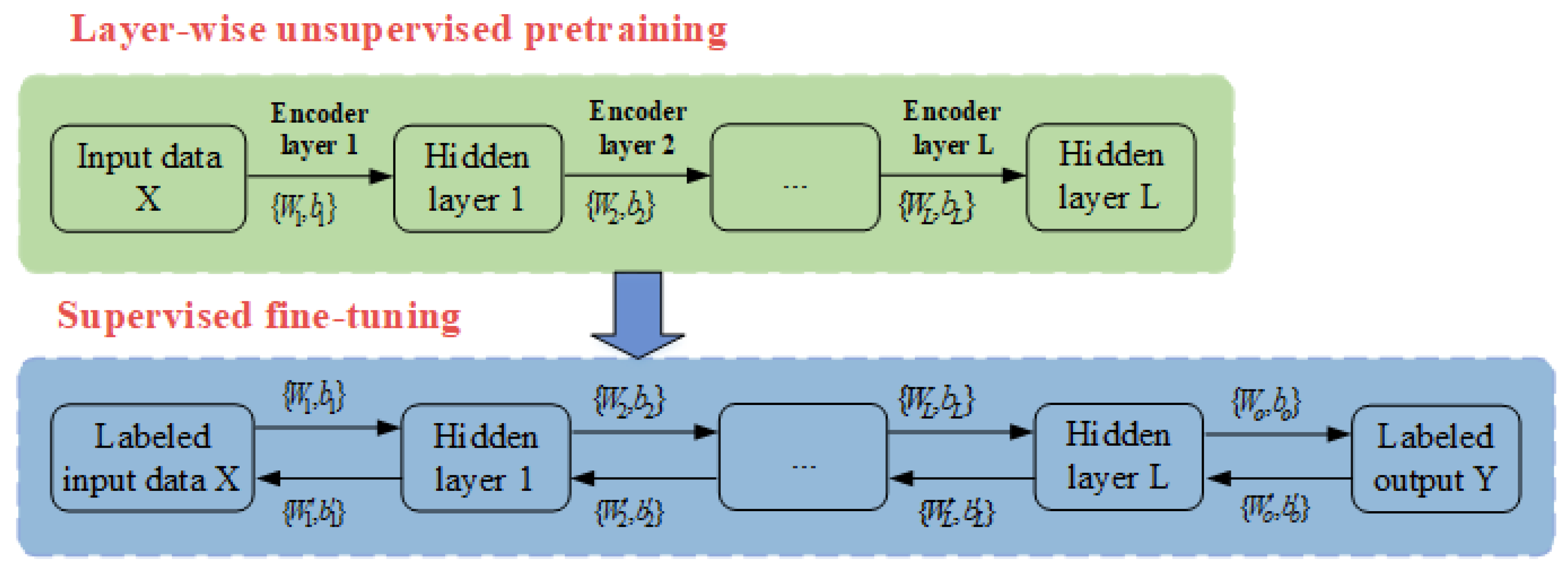
• A health indicator (HI) constructor based on a SAE-DNN is developed. No manually extracted features are used in the construction of the SAE-DNN-based HI constructor. The SAE-DNN automatically extracts representative features during the training process.
• The constant false-alarm rate (CFAR) algorithm is used to capture the AE hits in every degradation cycle; the number of AE hits in each cycle is considered the label to train the DNN.
• The LSTM-RNN is investigated to learn the long-term dependencies of HI curves constructed in an offline process and is then used to predict the RUL of a concrete structure in an online process.

This paper is arranged as follows: Section 2 introduces the experimental setup with data descriptions and illustrations. Section 3 describes the SAE-DNN-based HI constructor thoroughly, along with the LSTM-RNN-oriented RUL prognosis. Section 4 gives the experimental results and analysis. Finally, Section 5 presents our conclusions.

2. Experimental Setup

2.1. Experimental Specimens and Data Acquisition System

All of the reinforced concrete (RC) beam specimens are identical in terms of specifications: 240 × 15 × 30 cm in length × width × height; compressive strength 24 MPa; and five reinforcing bars of 16-mm diameter (Figure 1). The maximum tensile strength for each specimen is over 455 MPa. To test our proposed approach, a run-to-failure dataset is constructed from four-point bending tests on the RC beams (Figure 2). Each four-point bending test is performed as follows: an RC beam is loaded equally with two concentrated loads. Supports are placed 2000 mm apart, center-to-center. The displacement rate applied by the actuator through the I-section of an 80-cm steel beam can be either 1 mm/s or 2 mm/s. This load is continuously applied on each RC beam until the beam is completely crushed. The vertical displacement is measured by a linear variable differential transformer (LVDT) located at the middle of the bottom surface (Figure 2).

Figure 1. Schematic illustration of longitudinal section and cross section of the RC beam.

Figure 2. Schematic illustration of the four-point bending test for the RC beam.

The data acquisition system is an eight-channel PCI-based AE system (PCI-8). This device is capable of simultaneous data acquisition, waveform processing, and data transfer up to 132 Mb/s in the 1–400 kHz range. Its channels are connected to eight low-frequency AE R3I-AST sensors mounted on the specimen’s surface. These sensors have outstanding sensitivity and require no extra preamplifier on the long cable drive. In order to ensure that the inherent characteristics of the concrete are omitted, the sampling rate of 5 MHz is set.

2.2. Separation of Destructive Processes

A conventional RUL prediction is based on the specimen’s deterioration progress. The progression of damage occurs as follows: the specimen shows high and stable performance during a long starting phase, which then begins to deteriorate gradually during the second period. In the final stage, the degradation intensifies and, as a consequence, the specimen’s performance plummets abruptly and drastically until its final failure.

In comparison, fracture monitoring separates crack growth into four stages, as shown in Figure 3:

Figure 3. Damage progression in an RC beam during a bending test.

• Stage 1: The RC specimen deteriorates from its normal condition to a damaged state. Micro-cracks start at the end of this stage.
• Stage 2: Hairline cracks appear on the surface, which soon develop into macro-cracks.
• Stage 3: Main cracks form. Distributed flexure appears along with shear cracks, which soon lead to steel yielding.
• Stage 4: The steel yielding intensifies and shear cracks ultimately culminate in concrete crushing.

The degradation process measured by sensor 1 of specimen 1 is shown in Figure 3 in terms of load and number of AE hits in 1-second signal cycles.

3. Methodologies

3.1. SAE-DNN-Based HI Constructor

The multiple hidden layers concept has been available since the early years of deep learning. This approach was initially disappointing because its performance was even worse than shallow networks, the result of the limitations of conventional back-propagation due to poor training, which often utilized random initialization and got stuck in unoptimized local solutions. This difficulty was overcome in 2006 with unsupervised layer-wise pretraining, which was proposed by Hinton et al. [28] to deal with the existing limitations of DNN optimization. Currently, more sophisticated and abstract features with hierarchical structures can be learned because pretraining offers layer-by-layer, high-level feature extraction from lower-level ones.

An excellent choice for an efficacious layer-wise unsupervised learning algorithm would be a stacked autoencoder (SAE) [29]. This structure includes multi-layer AEs, each of which is a single-hidden-layer unsupervised neural network, and its input/output layers are set identically. The original input is intended to be reconstructed by the output layer with high accuracy. A simplified AE structure is illustrated in Figure 4. The input of SAE, which is supposedly $x={[x_1,x_2,\dots ,x_n]}^T\in R^n$ with dimension $n$, is projected by the encoder to the hidden layer $h={[h_1,h_2,\dots ,h_m]}^T\in R^m$ by the following mapping function $f$:

$$h=f(x)=s_f(Wx+b)$$

(1)

in which $m$ stands for the dimension of the hidden variable vector; $W$ is the $m\times n$ weight matrix; $b\in R^m$ is the bias vector; and the nonlinear activation function $s_f$ can be either the sigmoid function, the tanh function, or the rectified linear unit function.

Figure 4. Model structure of AE.

The hidden representation $h$ is then mapped to the output layer $\tilde{x}\in R^n$ by the mapping function $\tilde{f}$ in the decoder:

$$\tilde{x}=\tilde{f}(h)=s_{\tilde{f}}(\tilde{W}h+\tilde{b})$$

(2)

with $\tilde{W}$ as an $n\times m$ weight matrix; $\tilde{b}\in R^n$ as the bias vector term for the output layer; and the activation function $s_{\tilde{f}}$ as either the sigmoid function or others. Overall, $\theta =\{W,\tilde{W},b,\tilde{b}\}$ is the AE parameter set and $g_{\theta }(x)=\tilde{f}(f(x))\approx x$ is the function to be learned. As aforementioned, an AE aims to get the reconstructed output $\tilde{x}$ as close to the initial input $x$ as possible. This is done by forcing constraints on the network, for example, a hidden unit number limitation. Assume that the training input is $X=\{x^{(1)},x^{(2)},\dots ,x^{(N)}\}$, where the total number of training samples is denoted as $N$. Initially, each $x^{(i)}$ is projected to a hidden representation $h^{(i)}$ and then mapped to the reconstructed data ${\tilde{x}}^{(i)}$. By the following mean squared reconstructed error calculation, the reconstructed loss function can be minimized:

$$\begin{array}{ll}J(W,\tilde{W},b,\tilde{b})& ={{\displaystyle \sum _{i=1}^N\Vert {\tilde{x}}^{(i)}-x^{(i)}\Vert }}^2/2N\\ & ={{\displaystyle \sum _{i=1}^N\Vert g_{\theta }(x^{(i)})-x^{(i)}\Vert }}^2/2N\end{array}$$

(3)

The gradient descent (GD) is used for AE parameter updating. After the completion of training, the weight and bias are then saved for this AE. The multi-AE-layered structure of an SAE is presented in Figure 5. The layer-by-layer training of an SAE is done as follows: Initially, the original input data is mapped in the first hidden feature layer by the first AE; the output of the first AE is then considered the input for the second AE, and the process continues. By the end, every layer in the SAE is pretrained. To prevent the AE from just learning the identity of the input and make the learnt features more robust, noise can be added to the input data for training. The AE is forced to reconstruct a corrupted version of the input. This method is called a stacked denoising autoencoder (SDA) and it is chosen for our study.

Figure 5. Training procedure of an SAE.

Following the unsupervised pretraining, the output layer is added to the top of the SAE and the weights and biases are fine-tuned. Each hidden layer’s weights are initialized by the pretrained weights ${\{W_k,b_k\}}_{k=1,2,\dots ,K}$. The output layer’s parameters $\{W_0,b_0\}$ can be set by random initialization. Afterwards, back-propagation is utilized to achieve improved weights ${\{W_k^{\prime },b_k^{\prime }\}}_{k=1,2,\dots ,K}$ by fine-tuning the entire network. The predicted error is minimized as follows:

$$J_o={{\displaystyle \sum _{j=1}^N\Vert y_j-{\widehat{y}}_j\Vert }}^2/2N$$

(4)

with $y_j$ and ${\widehat{y}}_j$ being the $j^{th}$ data sample’s label and predicted output, respectively. The SAE training procedure is displayed in Figure 5.

3.2. Impulse Detection Using the Constant False Alarm Rate (CFAR) Algorithm

In this study, impulse detection is performed with the CFAR algorithm. CFAR is a popular data-based target-detecting technique that excels in environments where background noise and interference are varying, especially for radar systems. A threshold based on power is determined so that when a signal segment exceeds it, this segment can be considered a “hit” on the target.

Most CFAR schemes utilize a power threshold calculated from the noise floor of the cell blocks surrounding the cell under test (CUT). Several cells adjacent to the CUT are neglected to protect the training cells from signal leaking, which can negatively influence the noise estimation. Figure 6 describes a simplified CFAR scheme.

Figure 6. Diagram of a CFAR detection scheme.

In this study, the cell average CFAR with acknowledged stability and robustness [30] is chosen for implementation. The threshold for detection $T$ is first computed as follows:

$$T_i=\alpha P_i$$

(5)

with $\alpha$ as the threshold factor and $P_i$ being the estimated noise power, as calculated:

$$P_i=\frac{1}{2N}{\displaystyle \sum _{\ell =G+1}^{G+N}{\left|C_{i+\ell }\right|}^2}+{\left|C_{i-\ell }\right|}^2$$

(6)

where $N$ and $G$ are the number of training cells and guard cells, respectively. Generally, the number of leading and lagging cells are set as equal. The threshold factor $\alpha$ is harnessed to control the number of detected targets in a directly proportional relationship:

$$\alpha =N(P_{fa}^{-1/N}-1)$$

(7)

with $P_{fa}$ being the desired false alarm rate. This parameter should be chosen with caution, since it is a trade-off between the number of detected targets and the number of detected false targets.

This study deals with signals in one-second segments, each of which is then divided into 2000 cells for analysis. Both leading and lagging blocks contain 30 cells, in which 20 are used for training and the rest are guard cells. Equations (5)–(7) are used to calculate the adaptive threshold of each CUT. A target is detected when the power of the CUT exceeds its threshold. The concept and results of this algorithm are shown in Figure 7.

Figure 7. The application of CFAR detection for impulse detection. (a) Power of cells versus adaptive threshold, (b) AE impulse automatically picked during 1-second length.

3.3. LSTM-RNN-Oriented RLU Prediction

LSTM has been adopted as a popular solution for temporal sequence and long-range dependency modeling, having been applied in numerous studies on language modeling, speech recognition, and online handwriting recognition, among others. The reason for the preference of LSTM over RNN is its ability to resolve the vanishing/exploding gradients inherent in RNN training. Figure 8 presents LTSM in its basic structure, with the number of input layers, recurrent layers, and output layers all being 1. The innovation of LSTM is that it introduces different types of gates, such as the input gate $i_{(t)}$, forget gate $f_{(t)}$, output gate $o_{(t)}$, and input modulation gate $g_{(t)}$, and other components like hidden units $h_{(t)}$ and memory cells $c_{(t)}$.

Figure 8. LSTM cell.

Information disposing is determined and performed by the forget gate $f_{(t)}$. This gate utilizes a logistic activation function for inputs $x_{(t)}$ and $h_{(t-1)}$, of which the output is then provided to an element-wise multiplication operation. The gate is closed if the output is 0, and open if it is 1. The forget gate’s calculation is:

$$f_t=\sigma (W_{xf}{x}_t+W_{hf}{h}_{t-1}+b_f)$$

(8)

Afterwards, new information is evaluated to decide whether it can be stored in the internal state. Initially, the “input modulation gate” $g_{(t)}$, which acts as a tanh layer, forms a candidate state vector $c_{(t)}$. Then, the input gate $i_{(t)}$ determines which parts of $g_{(t)}$ are to be supplemented to the long-term state $c_{(t)}$. The two outputs are computed as follows:

$$i_{(t)}=\sigma (W_{xi}{x}_{(t)}+W_{hi}{h}_{(t-1)}+b_i)$$

(9)

$$g_{(t)}=\tanh (W_{xg}{x}_{(t)}+W_{hg}{h}_{(t-1)}+b_g)$$

(10)

Deriving from Equations (8)–(10), the previous internal state $c_{(t-1)}$ can be used to achieve the current state $c_{(t)}$:

$$c_{(t)}=f_{(t)}\otimes c_{(t-1)}+i_{(t)}\otimes g_{(t)}$$

(11)

Eventually, the long-term state is then evaluated by the output gate $o_{(t)}$ to determine which parts of it can be read and output at this time to both $h_{(t)}$ and $y_{(t)}$. After putting the internal state $c_{(t)}$ through a tanh layer (to push the values to be between −1 and 1), it is multiplied by the output of the sigmoid gate to acquire the remaining state values. This is calculated as follows:

$$o_{(t)}=\sigma (W_{xo}{x}_{(t)}+W_{ho}{h}_{(t-1)}+b_o)$$

(12)

$$y_{(t)}=h_{(t)}=o_{(t)}\otimes \tanh (c_{(t)})$$

(13)

with W and b as the layer weights and biases, respectively.

4. Experimental Validation

4.1. Dataset Description

Figure 9 displays the four-point bending test from which the dataset used here was collected. Our proposed method is validated on AE data acquired by AE sensors at the sampling frequency of 5 MHz. The duration of each degradation cycle is set at 1 s. For each four-point bending test, a total of eight sensors are positioned on the RC beam to collect data in the run-to-failure process.

Figure 9. Pictogram of the four-point bending test.

Twenty-four run-to-failure process signals are acquired during three four-point bending tests to validate the proposed approach. Details about the dataset are listed in Table 1. The data is divided into two equal parts for training (signals from sensors 1–4) and test sets (signals from sensors 5–8) formation. Figure 10 shows the degradation process of three test run-to-failure sensor signals (i.e., sensor 5), one from each of the concrete beams, in terms of RMS, kurtosis values, and AE hits.

Table 1. Specifics of the experimental dataset.

Dataset	Bending Test	Concrete Beam	No. Sensors (Run-to-Fail Signals)	Signal Length (s)
Training dataset	1	A	4	600
	2	B	4	650
	3	C	4	620
Test dataset	1	A	4	600
	2	B	4	650
	3	C	4	620

Figure 10. Illustration of the degradation process of concrete beams using RMS values, kurtosis values and AE hits.

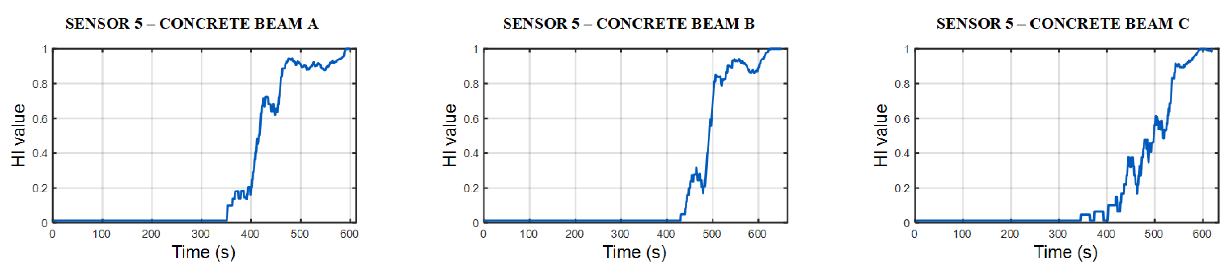
4.2. The Efficacy of an SAE-DNN-Based HI Constructor

This stage starts with SAE-DNN-based HI constructor training. Initially, fast Fourier transform (FFT) is utilized to determine the signal segment’s spectrum. Since each segment is 5 × 10⁶ in length, after FFT there are 2.5 × 10⁶ data points which are too big to feed into the SAE. Therefore, the number of inputs is reduced by splitting the spectrum of the AE signals into a suitable amount of frequency bands and then computing their root mean square (RMS), which represents an approximation of each band’s energy.

Following the data preprocessing, the SAE model is constructed and trained. Signal spectrum vectors of size 2000 are fed to the encoder, which are then processed by three size-diminishing dense layers (1000 to 200 to 10 units with Xavier initialization and the ELU activation function). The encoder’s output (size of 10) is then fed to the decoder and processed by three size-increasing dense layers (200 to 1000 to 2000 units). Dropout layers with rate of 0.1 are added before the dense layers to improve the SAE’s regularization. Afterwards, Adam optimization is utilized for SAE training with unlabeled signal spectra as both the inputs and targets. Different levels (from 0.1–0.5) of the fractions of masked zero are tested, which shows the best performance at 0.1.

Then the encoder’s layers are reused in the DNN model as the hidden layers. After a logistic regression layer addition, this DNN model is fine-tuned in a supervised way. The DNN output layer’s size is 1 and its according label is the normalized number (in the range of [0, 1]) of AE hits detected in each degradation cycle. The DNN model is designed so that the outputs, which are the HI values, are in the range of [0, 1], therefore the sigmoid activation is chosen as the activation function of the output layer. During the training process, the reused layers are frozen so that they retain the learning ability of high-level features from the low-level input features of the SAE model. In addition, the early stopping and checkpoint techniques are applied during training SAE and DNN to get the best parameters of SAE and DNN structures.

Following the completion of SAE-DNN-based HI constructor’s training, the run-to-failure data is harnessed for the concrete beam’s HI construction. Half of the signals are utilized here for the evaluation of the HI constructor’s performance. Figure 11 shows the HIs of the three tests from sensor 5. In comparison to HIs constructed from conventional features like RMS and kurtosis with larger scales, the proposed method’s HIs ranges between 0 and 1, with 1 being the failure condition. Consequently, the threshold definition has no need for such HI employment. An HI exceeding a fixed FT triggers the obtain of RUL.

Figure 11. HIs of test datasets constructed by the proposed model for concrete beam A, B, and C.

Two other metrics, monotonicity and trendability, [24] are also used in this study for HI fitness validation. Monotonicity is the characterization of the underlying increasing or decreasing trend:

$$M=\left|\frac{no.of.d/dx>0}{n-1}-\frac{no.of.d/dx<0}{n-1}\right|$$

(14)

with n being the number of observations for a specific feature. Monotonicity $M$ can be calculated with the absolute difference between a feature’s “positive” and “negative” derivatives. It ranges from 0–1, with 0 emphasizing a non-monotonic feature and 1 showing a highly monotonic feature.

The second metric, trendability, is related to an extracted feature’s functional form and correlation with time. In another words, it shows how an asset’s state varies with time. For example, a constant function presents zero correlation with time, while a high correlation can be found with a linear function. Similarly, non-linearity also causes a variation in correlation. This metric is computed as follows:

$$R=\frac{n\left({\displaystyle \sum xy}\right)-\left({\displaystyle \sum x}\right)\left({\displaystyle \sum y}\right)}{\sqrt{\left[n{\displaystyle \sum x^2-{\left({\displaystyle \sum x}\right)}^2}\right]\left[n{\displaystyle \sum y^2-{\left({\displaystyle \sum y}\right)}^2}\right]}}$$

(15)

with $R$ being the correlation coefficient between $x$ and $y$, which are the feature and time index, respectively, in this study. The state of correlation can be either no correlation, negative, positive, or perfect. Thus, $R$ ranges from −1 to 1. Figure 12 shows a conceptual demonstration of the curve fits.

Figure 12. Definition of curve fitness metrics.

With the aim to highlight the improvement of the proposed method’s HIs compared to HIs based on RMS or kurtosis, a fitness analysis is done on the testing dataset. In this analysis, two aforementioned metrics of each type of HI are measured. Table 2 shows the summarized results, in which the proposed method presents a significant boost of performance in comparison with the two HIs based on RMS and kurtosis. This implies that our method is more suitable in terms of describing the concrete beam degradation process.

Table 2. Metric comparison of different types of HIs.

Type of HI	Min Value	Max Value	M	R
RMS	0.0005	0.1529	0.037 ± 0.022	0.347 ± 0.064
Kurtosis	2.7496	5629.1	0.004 ± 0.021	0.458 ± 0.050
Crest factor	3.0803	145.91	0.0013 ± 0.183	0.7416 ± 0.024
Skewness	−19.279	10.855	0.0102 ± 0.0215	0.1077 ± 0.1020
Entropy	0.0883	4.8324	0.0019 ± 0.0234	0.1886 ± 0.1740
SAE-DNN	0.0125	1	0.6788 ± 0.079	0.6801 ± 0.0489

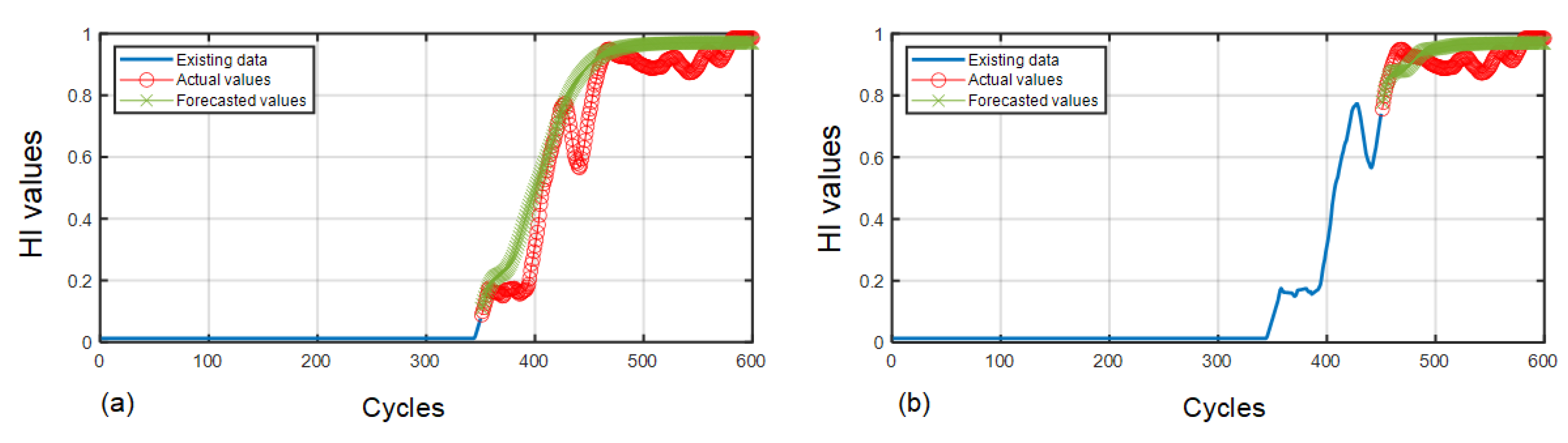
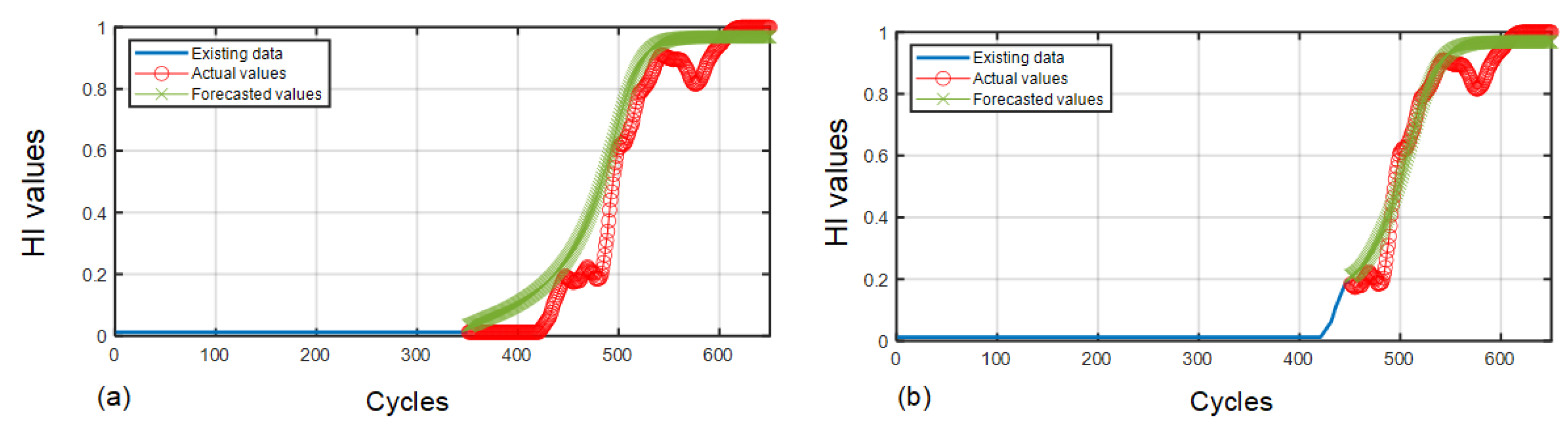
4.3. The Efficacy of the LSTM-RNN-Oriented RLU Prediction

The LSTM-RNN-based RLU predictor is then trained with previously constructed HI curves, which are segmented into a series of time-steps. The data can be considered a univariate time series due to it being a sequence of one value per time step. The RUL predictor utilizes past HI values to predict the future ones until a predefined threshold is met. In order to maximize the number of time series to train the model, a shifting window of size 50 is used in the segmentation process. This procedure is shown in Figure 13.

Figure 13. Time series construction from training degradation data.

At this step the LSTM predictor is already capable of forecasting the next time-step value. However, with an alteration in the procedure, it can also predict more than just one future state. The next prediction can be added to the inputs (acting as if this predicted value had occurred) to further predict the following ones until the end. Our model is trained to forecast at every time-step instead of just the final time-step. By following this technique, the loss can contain a term for every time-step output rather than just the output at the last time step. This allows more stabilization and faster training as more error gradients are able to flow through the model [22].

One input layer of the same size as the number of time-steps is utilized for the construction of the applied LSTM-RNN. Following this layer are two hidden LSTM layers of size 20. A linear activation function is utilized in the dense output layer of one neuron. Early stopping and checkpoint techniques are also used during training to construct a better LSTM-RNN model.

The developed method is implemented with degradation data collected from three concrete beams A, B, and C. Generally, RUL estimations toward the end of a degradation process are more important than earlier ones because this is usually when maintenance decisions are made. Therefore, two major time stamps at cycle 350 (minor crack initialization) and cycle 450 (major crack initialization) are chosen for the average prediction error calculation. The definition of the RUL prediction error is:

$$\overline{e}=\left|L{C}_i-\widehat{L{C}_i}\right|$$

(16)

with $\overline{e}$ being the RUL prediction error, and $L{C}_i$, $\widehat{L{C}_i}$ are the actual cycles and the estimated cycles, respectively.

In this study, the DNN model is designed so that the outputs, which are the HI values, are in the range of [0, 1]. Therefore, the sigmoid activation is chosen as the activation function of the output layer. In this case, the fixed HI threshold should be set to 1. However, experimental results have shown that the output of DNN rarely reaches the value of 1. Hence, this study has set the fixed HI threshold of 0.95 to mark the specimen’s breakdown.

Figure 14 shows specimen A’s RUL prediction error with the prediction calculated at cycle 350, and the prediction error calculated at cycle 450. The details of statistics concerning specimen A’s RUL prediction error can be found in Table 3 along with the other two specimens; a minor prediction error with a small standard deviation is preferred. As can be seen in Table 3, the proposed method’s prediction error at cycle 350 is 32 cycles, which is lower than the error of 36 and 81 cycles predicted by the gated recurrent unit (GRU) RNN [31] and the simple RNN, respectively. This indicates that our method is more effective at capturing long-term dependencies than those other two approaches. The prediction error at cycle 450 is 21, 32, and 61 cycles, respectively. It is clear that, in both cases, the simple RNN presents the largest error. This is ample evidence showing its inability to effectively store and learn long-term dependencies without special gates.

Figure 14. LSTM-RNN-based RLU prediction results of concrete beam A: (a) at cycle 350; (b) at cycle 450.

Table 3. RUL prediction results.

Fault-to-Failure Signals	Method	Prediction Error Cycles (at Cycle 350)	Prediction Error Cycles (at Cycle 450)
Concrete beam A	LSTM-RNN	32 ± 3	21 ± 4
	GRU-RNN *	36 ± 4	32 ± 5
	Simple RNN	81 ± 6	61 ± 8
Concrete beam B	LSTM-RNN	41 ± 7	34 ± 5
	GRU-RNN *	43 ± 6	37 ± 7
	Simple RNN	95 ± 11	89 ± 8
Concrete beam C	LSTM-RNN	36 ± 3	24± 3
	GRU-RNN *	39 ± 7	32 ± 3
	Simple RNN	88 ± 4	68 ± 7

* Gated recurrent unit RNN [31].

The proposed method’s results on specimen B are shown in Figure 15. The prediction error of our proposed LSTM-RNN, the GRU-RNN, and the simple RNN at cycle 350 were 41, 43, and 95 cycles, respectively. At cycle 450, they were 34, 37, and 89 cycles.

Figure 15. LSTM-RNN-based RLU prediction results of concrete beam B: (a) at cycle 350; (b) at cycle 450.

In Figure 16, specimen C’s prediction results from the proposed method are plotted; its values can be again checked in Table 3. The first prediction at cycle 350 shows the prediction error for our proposed method and the GRU-RNN as 36 and 39 cycles, respectively; the prediction error at cycle 450 are 24 cycles with LSTM-RNN and 32 cycles with GRU-RNN. Concerning the simple RNN, the 88 and 68 divergent cycles in the two predictions clearly demonstrate its failure of long-term dependencies learning.

Figure 16. LSTM-RNN-based RLU prediction results of concrete beam C: (a) at cycle 350; (b) at cycle 450.

5. Conclusions

Reliable HI curves construction and long-term dependencies learning of degradation data are important but challenging tasks for an accurate remaining useful life (RUL) estimation of concrete structures. In this study, we proposed an SAE-DNN model that automatically constructs HI curves from degradation raw signals. The HI curves constructed have better fitness metrics than statistical parameters-based HI curves. More specifically, these HI curves have the average monotonicity and trendability metrics of 0.67 and 0.68, respectively, which much higher than those of HI curves based on statistical parameters such as RMS, Kurtosis, or Sknewness, etc. Moreover, the curves’ HI values are in the range of a [0, 1], therefore, threshold definition is no need for such HI employment.

The HI curves constructed from training degradation data are then fed to train the LSTM-RNN for RUL prediction. The study validates the prediction performance of the LSTM-RNN by estimating RUL and calculating the average prediction error on testing experimental concrete beams at two times; at cycle 350 (minor crack initialization) and at cycle 450 (major crack initialization). Experimental results on concrete beams A, B, and C indicate that the LSTM-RNN generally estimates more accurate RULs of concrete beams than the GRU-RNN and the simple RNN. The average prediction error cycles of the LSTM-RNN on concrete beams A, B, C at cycle 350 are 32, 41, and 36, respectively; at cycle 450 are 21, 34, 24, respectively. These error values are lower than those of the GRU-RNN and much lower than those of the simple RNN. In other words, the proposed method outperformed a GRU-RNN and a simple RNN in predicting the RUL of concrete structures.

Overfitting is an important issue that needs to be handled carefully during training deep neural networks, especially when the data training is limited as in this study. It makes the outcome of deep neural networks low and unstable. There are currently many techniques to help neural networks avoid overfitting such as L1 and L2 regularization, Monte Carlo dropout, etc. In the upcoming times, our focus is to dig deep into these techniques to find the best one for our model.

References

- Ohno, K.; Ohtsu, M. Crack classification in concrete based on acoustic emission. Construct. Build. Mater. 2010, 24, 2339–2346. [Google Scholar] [CrossRef]
- Aggelis, D.G. Classification of cracking mode in concrete by acoustic emission parameters. Mechan. Res. Commun. 2011, 38, 153–157. [Google Scholar] [CrossRef]
- Aggelis, D.; Mpalaskas, A.; Matikas, T. Investigation of different fracture modes in cement-based materials by acoustic emission. Cement Concr. Res. 2013, 48, 1–8. [Google Scholar] [CrossRef]
- Tra, V.; Kim, J.-Y.; Jeong, I.; Kim, J.-M. An acoustic emission technique for crack modes classification in concrete structures. Sustainability 2020, 12, 6724. [Google Scholar] [CrossRef]
- Fan, S.-K.S.; Hsu, C.-Y.; Tsai, D.-M.; He, F.; Cheng, C.-C. Data-driven approach for fault detection and diagnostic in semiconductor manufacturing. IEEE Trans. Autom. Sci. Eng. 2020, 17, 1925–1936. [Google Scholar] [CrossRef]
- Fan, S.-K.S.; Hsu, C.-Y.; Jen, C.-H.; Chen, K.-L.; Juan, L.-T. Defective wafer detection using a denoising autoencoder for semiconductor manufacturing processes. Adv. Eng. Inf. 2020, 46, 101166. [Google Scholar] [CrossRef]
- Park, Y.-J.; Fan, S.-K.S.; Hsu, C.-Y. A Review on Fault Detection and Process Diagnostics in Industrial Processes. Processes 2020, 8, 1123. [Google Scholar] [CrossRef]
- Phi Duong, B.; Kim, J.-M. Prognosis of remaining bearing life with vibration signals using a sequential Monte Carlo framework. J. Acoust. Soc. Am. 2019, 146, EL358–EL363. [Google Scholar] [CrossRef]
- Xia, M.; Li, T.; Shu, T.; Wan, J.; De Silva, C.W.; Wang, Z. A two-stage approach for the remaining useful life prediction of bearings using deep neural networks. IEEE Trans. Ind. Inf. 2018, 15, 3703–3711. [Google Scholar] [CrossRef]
- Wang, Y.; Peng, Y.; Zi, Y.; Jin, X.; Tsui, K.-L. A two-stage data-driven-based prognostic approach for bearing degradation problem. IEEE Trans. Ind. Inf. 2016, 12, 924–932. [Google Scholar] [CrossRef]
- Gao, Z.; Cecati, C.; Ding, S.X. A survey of fault diagnosis and fault-tolerant techniques—Part I: Fault diagnosis with model-based and signal-based approaches. IEEE Trans. Ind. Electr. 2015, 62, 3757–3767. [Google Scholar] [CrossRef]
- Yin, S.; Ding, S.X.; Xie, X.; Luo, H. A review on basic data-driven approaches for industrial process monitoring. IEEE Trans. Ind. Electr. 2014, 61, 6418–6428. [Google Scholar] [CrossRef]
- Tra, V.; Khan, S.A.; Kim, J.-M. Diagnosis of bearing defects under variable speed conditions using energy distribution maps of acoustic emission spectra and convolutional neural networks. J. Acoust. Soc. Am. 2018, 144, EL322–EL327. [Google Scholar] [CrossRef]
- Tra, V.; Kim, J. Pressure Vessel Diagnosis by Eliminating Undesired Signal Sources and Incorporating GA-Based Fault Feature Evaluation. IEEE Access 2020, 8, 134653–134667. [Google Scholar] [CrossRef]
- Tra, V.; Kim, J.; Khan, S.A.; Kim, J.-M. Incipient fault diagnosis in bearings under variable speed conditions using multiresolution analysis and a weighted committee machine. J. Acoust. Soc. Am. 2017, 142, EL35–EL41. [Google Scholar] [CrossRef] [PubMed]
- Williams, T.; Ribadeneira, X.; Billington, S.; Kurfess, T. Rolling element bearing diagnostics in run-to-failure lifetime testing. Mechan. Syst. Sig. Proc. 2001, 15, 979–993. [Google Scholar] [CrossRef]
- Antoni, J. The spectral kurtosis: A useful tool for characterising non-stationary signals. Mech. Syst. Sig. Proc. 2006, 20, 282–307. [Google Scholar] [CrossRef]
- Bozchalooi, I.S.; Liang, M. A smoothness index-guided approach to wavelet parameter selection in signal de-noising and fault detection. J. Sound Vib. 2007, 308, 246–267. [Google Scholar] [CrossRef]
- Guo, L.; Li, N.; Jia, F.; Lei, Y.; Lin, J. A recurrent neural network based health indicator for remaining useful life prediction of bearings. Neurocomputing 2017, 240, 98–109. [Google Scholar] [CrossRef]
- Wang, D.; Peter, W.T.; Guo, W.; Miao, Q. Support vector data description for fusion of multiple health indicators for enhancing gearbox fault diagnosis and prognosis. Meas. Sci. Technol. 2010, 22, 025102. [Google Scholar] [CrossRef]
- Tra, V.; Kim, J.; Khan, S.A.; Kim, J.-M. Bearing fault diagnosis under variable speed using convolutional neural networks and the stochastic diagonal levenberg-marquardt algorithm. Sensors 2017, 17, 2834. [Google Scholar] [CrossRef] [PubMed]
- Géron, A. Hands-On Machine Learning with Scikit-Learn, Keras, and Tensor Flow: Concepts, Tools, and Techniques to Build Intelligent Systems; O’Reilly Media: Newton, MA, USA, 2019. [Google Scholar]
- Zhang, Y.; Xiong, R.; He, H.; Pecht, M.G. Long short-term memory recurrent neural network for remaining useful life prediction of lithium-ion batteries. IEEE Trans. Veh. Technol. 2018, 67, 5695–5705. [Google Scholar] [CrossRef]
- Zhao, R.; Yan, R.; Wang, J.; Mao, K. Learning to monitor machine health with convolutional bi-directional LSTM networks. Sensors 2017, 17, 273. [Google Scholar] [CrossRef] [PubMed]
- Zhang, T.; Song, S.; Li, S.; Ma, L.; Pan, S.; Han, L. Research on gas concentration prediction models based on LSTM multidimensional time series. Energies 2019, 12, 161. [Google Scholar] [CrossRef]
- Liu, J.; Zhang, T.; Han, G.; Gou, Y. TD-LSTM: Temporal dependence-based LSTM networks for marine temperature prediction. Sensors 2018, 18, 3797. [Google Scholar] [CrossRef]
- Liu, Y.; Guan, L.; Hou, C.; Han, H.; Liu, Z.; Sun, Y.; Zheng, M. Wind power short-term prediction based on LSTM and discrete wavelet transform. Appl. Sci. 2019, 9, 1108. [Google Scholar] [CrossRef]
- Hinton, G.E.; Osindero, S.; Teh, Y.-W. A fast learning algorithm for deep belief nets. Neural Comput. 2006, 18, 1527–1554. [Google Scholar] [CrossRef]
- Yuan, X.; Huang, B.; Wang, Y.; Yang, C.; Gui, W. Deep learning-based feature representation and its application for soft sensor modeling with variable-wise weighted SAE. IEEE Trans. Ind. Inf. 2018, 14, 3235–3243. [Google Scholar] [CrossRef]
- Richards, M.A. Fundamentals of Radar Signal Processing; Tata McGraw-Hill Education: New York, NY, USA, 2005. [Google Scholar]
- Cho, K.; Van Merriënboer, B.; Gulcehre, C.; Bahdanau, D.; Bougares, F.; Schwenk, H.; Bengio, Y. Learning phrase representations using RNN encoder-decoder for statistical machine translation. arXiv 2014, arXiv:1406.1078. [Google Scholar]
Publisher’s Note: MDPI stays neutral with regard to jurisdictional claims in published maps and institutional affiliations. |
© 2021 by the authors. Licensee MDPI, Basel, Switzerland. This article is an open access article distributed under the terms and conditions of the Creative Commons Attribution (CC BY) license (https://creativecommons.org/licenses/by/4.0/).