Abstract
This paper concerns the algorithm of transition piezoelectric elements for adaptive analysis of electro-mechanical systems. In addition, effectivity of the proposed elements in such an analysis is presented. The elements under consideration are assigned for joining basic elements which correspond to the mechanical models of either the first or higher order, while the electric model is of arbitrary order. In this work, three variants of the transition models are applied. The first one assures continuity of displacements between the basic models and continuity of electric potential between these models, as well. The second transition piezoelectric model guarantees additional continuity of the stress field between the basic models. The third transition model additionally enables continuous change of the strain state between the basic models. Based on the mentioned models, three types of the corresponding transition finite elements are introduced. The applied finite element approximations are -adaptive ones, which allows element-wise changes of the element size parameter h, and the element longitudinal and transverse orders of approximation, respectively, p and q, depending on the error level. Numerical effectiveness of the models and their approximations is investigated in the contexts of: ability to remove high stress gradients between the basic and transition models, and convergence of the numerical solutions for the model problems of piezoelectrics with and without the proposed transition elements.
1. Introduction
More and more common application of piezoelectrics in contemporary technology requires more and more efficient and accurate methods of their modeling and analysis. In this work, we develop the new transition elements which possess unique set of features enabling joining mechanical shell models of the first order and higher orders. Such models are incompatible due to the assumptions of the plane stresses and no elongation of the normals to the shell mid-surface, both present in the first-order model. In order to join such models, the transition models are necessary. This refers also to the piezoelectricity case, when the mechanical field modeling needs simultaneous application of the first- and higher-order mechanical models.
Adaptive capabilities of -type are the second important feature of the new elements, where h is the element size parameter, while p and q are the element longitudinal and transverse orders of approximation. As our implementation of these capabilities is based on the standard -approximation rules, presented, respectively, in Reference [1,2] for 2D and 3D, we will not elucidate this aspect in this paper.
1.1. State of the Art
To the best of the authors’ knowledge, the transition piezoelectric elements have not been proposed yet, both in the classical (non-adaptive) and adaptive versions. Because of this, our literature survey can only be focused on two topics closest to the paper theme. The first topic concerns mathematical models of piezoelectrics and their finite element approximations. The second topic is the elastic transition models and the corresponding finite element approximations, as well.
1.1.1. Piezoelectric Models, Approximations and Finite Elements
Low-Order Models and Elements for Monolithic Piezoelectrics
Let us start this brief survey with the first-order and second-order models of piezoelectricity, where the model order concerns transverse displacement and electric potential fields. In Reference [3], the authors present classical (non-adaptive) finite element approximation and its features for the two-dimensional conventional (mid-surface unknowns) Reissner-Mindlin piezoelectric plate model including membrane effects. The finite element approximation is of mixed type with shear stresses treated as independent unknowns. The Kirhchoff piezoelectric plate model can be obtained as a special case. The latter model was also analyzed in Reference [4]. The simple flat shell element based on the conventional (mid-surface) displacements, rotations, and electric potential for plane stress and neglect of the in-plane electric field and electric displacements is presented in Reference [5]. The element is based on the assumed natural strain formulation in order to overcome numerical locking phenomena. Subsequently, in Reference [6], the Reissner-Mindlin mechanical model is combined with the first-order and second-order electric potential field in the transverse directions. Two formulations are applied, the displacement-like and hybrid with the electric displacements treated as independent unknowns. In Reference [7], the second-order transverse mechanical field is applied in the frame of three-dimensional elasticity for thin-walled piezoelectric plates. The electric potential field is also of the second-order in the transverse direction. The balanced reduced integration is applied as a numerical technique which serves removing the locking phenomena. The analytical conventional model of the Reissner-Mindlin plates with non-constant electric field distribution is presented in Reference [8].
Hierarchical Models and Elements for Monolithic Piezoelectrics
The hierarchical two-dimensional conventional (mid-surface unknowns) models of piezoelectric plates were introduced and mathematically substantiated in Reference [9]. The mixed formulation is applied there with stresses and electric displacements completing displacements and electric potential. Carrera and co-workers [10] proposed hierarchic plate models up to the fourth-order. The formulation is displacement-based in the case of the higher-order models, and mixed in the case of the Reissner-Mindlin model. The models employ three-dimensional degrees of freedom (dofs) for the top and bottom surfaces, and conventional (mid-surface) higher-order dofs. In addition, a thermal field can be included into this formulation. In Reference [11], the 3D-based (three-dimensional unknowns only) piezoelectric hierarchy of solid, first-order (Reissner-Mindlin) and hierarchical shell, and solid-to-shell and shell-to-shell transition piezoelectric models are formulated. Their -adaptive finite element approximations are presented in Reference [12]. The formulation is displacement-like with displacements and electric potential as unknowns of the problem. In the case of the electric field, this approach allows for the three-dimensional and 3D-based symmetric-thickness models of dielectricity. The approach is based on the 3D-based hierarchical models [13] and approximations [14] for elasticity, and the corresponding models [15] and approximations [16] for dielectricity.
Models for Piezoelectric Composites
In the case of laminated piezoelectric structures, it is worth mentioning the following works. In Reference [17], the authors presented Reissner-Mindlin-type composite plate model with piezoelectric layers. The direct piezoelectric and pyroelectric effects are taken into account. In turn, the work of Reference [18] proposed the plain strain shell model with higher-order shear and normal deformation effects for analysis of cylindrical laminated piezoelectric shells with actuating and sensing piezoelectric layers. The work of Reference [6], mentioned in the context of the monolithic piezoelectrics, should be mentioned here as applied to tree-layered shell structures with two outer piezoelectric layers and an electrically neutral core. A similar sandwich plate structures are modeled as two Reissner-Mindlin piezoelectric layers and one neutral layer of the same character [19], with the mid-surface interdependent displacement dofs. The electric fields are of mixed character and are defined by the outer layers’ mid-surface electric potentials and independent electric field mid-surface values of the outer layers. In order to remove locking, the reduced integration method is applied. The generalized analytical Reissner-Mindlin model of laminated piezoelectrics was presented in Reference [21]. It allows analyses of the problems where the electric potential is not prescribed through the thickness. The method assumes small thickness and thus allows decomposition of the three-dimensional Reissner-Mindlin description into two-dimensional in-plane and one-dimensional through-the-thickness problems. Subsequently, the already cited work of Reference [10] concerning hierarchical models of single layered piezoelectrics can also be applied to the numerical analysis of hierarchically modeled multilayered structures, with piezoelectric layers included. The recent example [22] of analysis of multilayered shells concerns the first-order model of the functionally graded layers. In turn, the piece-wise second-order finite element model for multilayered structures with delamination and debonding was proposed in Reference [23].
1.1.2. Transition Piezoelectric, Dielectric and Elastic Models And Elements
Transition Elements for Three Physical Classes of Problems
It can be concluded from the previous subsection that the piezoelectric transition models and elements that serve joining the three-dimensional (or hierarchical shell) piezoelectric models with the first-order piezoelectric model are rare. The only works, which we have cited, concern the idea [15] and variational [11] and finite element [12] formulations of the same classical transition piezoelectric model and element. They guarantee continuity of the displacement and transverse deformation fields between the mentioned models. They also guarantee continuity of the electric potential between the piezoelectric models.
In Reference [16], it has been demonstrated that, in the case of dielectric field of electric potential used in electrostatics, no transition elements between the three-dimensional model and symmetric-thickness hierarchical models of the first and higher orders are necessary if the consistent finite element approximations of non-adaptive or adaptive character are applied. This is because the same definition of electric field (intensity) is applied within both dielectric models.
In the case of the elastic mechanical fields, two groups of the transition models can be distinguished. The first one guarantees continuity of the inconsistent generalized displacement fields of the neighboring models. In such inconsistent models, the kinematic unknowns are different or of different order, e.g., in the transverse direction. In the second group, additionally the definitions of the derivatives of the kinematic unknowns, e.g., strains and/or stresses, are different in the neighboring models and the corresponding finite elements. In this context, one may deal with the neighborhood of the three-dimensional elasticity and shell or plate theories, the three-dimensional theory, and beam or truss theories, as well as the shell/plate theories and the one-dimensional theories of beams or trusses. Due to the paper scope, only the first case will be elucidated here. A general review, including all three cases, can be found in the thesis [24].
Non-Adaptive Transition Elements for Elasticity
We start with the transition elements of the classical (non-adaptive) finite element methods where the neighboring elements are joined through the sides of the same size and finite element interpolations on these sides are consistent. In addition, location of three-dimensional, shell/plate, and transition domains is fixed and strictly determined by the structure geometry. The first examples of the transition elements of this type can be attributed to Surana [25], who took into account the consideration of Ahmad [26] on thick shell elements and his own research [27] on general and axi-symmetric shell elements. The work, in Reference [25], of Surana presents solid-to-shell elements which enable joining the thick-shell element with the linear, quadratic or cubic solid elements. The elements possess the bigger shell part equipped with the mid-surface dofs, and the smaller solid part limited to one side of the element and equipped with the tree-dimensional dofs. Plane stress is assumed in the entire transition element. Applications of the elements of this type to axi-symmetric [28] and three-dimensional [29] problems are presented. Extension onto thermo-mechanical analysis was done in Reference [30]. Note that the independent research of Bathe and Bolourchi [31], based on the mentioned work of Ahmad, led to the analogous transition elements. Gmür and Schorderet [32] suggested application of the three-dimensional or plane stress states in the Surana’s element depending on the geometrical shape of the domain the element is located in. Liao and others [33] extended application of the Surana’s elements onto laminated composite structures. Both, the shell and solid parts of the transition element are modeled as such composites. In the work of Reference [34], in order to avoid the numerical locking, the method based on strain interpolation (with the points where the strain values are known) was applied instead of the reduced integration.
In the work of Dávila [35], the opposite idea is applied, i.e., the elements consist of the larger solid part and smaller shell part. The latter part comprises one or two lateral sides. The top and bottom three-dimensional dofs and mid-surface dofs are applied within the solid and shell parts, respectively. Three-dimensional stress state is assumed throughout single-layered shells or each layer of composite shells. Yet another idea was suggested in Reference [36], by Gong, who proposed generalization of the solid-to-shell transition elements for the elements joining two-dimensional and three-dimensional elements. In this approach, the shell or two-dimensional parts consist of one or two lateral sides of the transition element. The longitudinal order of approximation can be higher than three. In the entire element, either three-dimensional or plane stress state can be applied.
Adaptive Transition Elements for Elasticity
In the case of the adaptive methods, finite elements of different sizes, orders of approximation (non-conforming approximations), and mechanical models are present in finite element meshes. In the case of different element sizes resulting from h-adaptivity based on remeshing, continuity of the field of unknowns may be based on introduction of the distorted elements on the boundaries between the mesh parts of various density. In the case of different sizes resulting from h-adaptivity based on local element refinement, continuity of the fields of unknowns requires introduction of the distorted elements [37] or is based on transition elements for monolithic [38] or multilayered [39] structures. Such transition elements deliver piece-wise linear [40] or approximate [41] continuity along the entire common edge or face, or at the common nodes only, e.g., within triangles [42], quadrilaterals [43] and hexahedrons [44]. Note that application of the smart idea of the constrained approximation, proposed by Demkowicz for 2D [1] and 3D [2], removes the necessity of introduction of the transition elements of this type as the continuity is automatically guaranteed by the constraints on the boundary between the elements of different sizes.
As far as the different approximation orders of the elements are concerned, transition elements may be introduced with the consistent approximation on the boundary between specific 2D [20] or general 3D [45] elements, with the continuity guaranteed again on the entire common edge or face, or at the common nodes only. A smart alternative is the idea of 2D [1] and 3D [2] hierarchical shape functions, defined independently in the element vertices, on its edges and sides, and in the interior of the element, which allows for the same approximation order on the common edge or face of the neighboring elements and different orders in their interiors.
In the case of different models of the neighboring elements, the continuity of the field of unknowns may require transition elements which conform the model of the larger number of nodal dofs with some of these dofs constrained to zero on the boundary with the model of the smaller number of nodal dofs. The 3D-2D [46], 2D-2D [47], and 2D-1D [48] versions of this approach can be found. The alternative is the transition elements equipped with the degrees of freedom of both models (see comments in Reference [49]). Note that such transition elements are not necessary if the uni-dimensional, e.g., three-dimensional, approach is applied within each of the neighboring models. The idea lies in using the same, e.g., three-dimensional, dofs for each model. This usually requires internal constraints in the model simplified (e.g., 3D-based shell models) with respect to the three-dimensional one. The linear [50] or higher [51] order of approximation can be applied in the transverse direction on the common face of the three-dimensional and 3D-based shell elements. Even though this technique guarantees continuity of the field of unknowns, high gradients of the derivatives on the boundary between the models appear. If one wants to get rid of such gradients, the transition elements removing stress [52] and, additionally, strain, Reference [24] gradients are necessary between the basic models being joined.
1.1.3. Conclusions
In this paper, we will use piezoelectric transition elements combining the ideas present in the following works concerning the uncoupled problem of elasticity. Firstly, we will apply the 3D-based approach [13], where the solid [53], hierarchical shell [14], first-order shell [54], and transition [51] models are equipped with the three-dimensional dofs only. This approach will also be extended onto the dielectricity models [16]. We will also apply the idea of Dávila [35], where one deals with larger 3D part and smaller thin-walled part of the transition element. The stress state within the element will be either three-dimensional, as in Reference [35], or transition (from three-dimensional to plane one) [24]. The -adaptive capabilities of the elements will be based solely on the ideas of Demkowicz and others [2]. Our 3D-based hierarchical finite element models will resemble the ideas presented, respectively, in Reference [55,56] for the cases of the three-dimensional and conventional (mid-surface) dofs.
1.2. The Scope and Novelty of the Paper
This paper concerns the algorithm of the solid-to-shell and shell-to-shell transition piezoelectric elements for adaptive analysis of electro-mechanical systems. Such systems can be composed of piezoelectric transducers and elastic structural elements, both of arbitrary shapes. In addition, effectivity of application of the proposed elements in such an analysis is of our interest in the paper. The elements are assigned for joining basic elements, namely piezoelectric shell elements of the first-order mechanical field and arbitrary-order electric field and piezoelectric elements of the hierarchical shell model (second- or higher-order) within the mechanical field and arbitrary-order within the electric field. Alternatively, the latter model can be replaced with the piezoelectric description based on hierarchical models of three-dimensional elasticity and three-dimensional dielectricity.
In this work, three variants of the transition models are applied. The first one, called classical, assures continuity of displacements between the basic models and continuity of electric potential between these models, as well. The second, modified transition piezoelectric model guarantees additional continuity of the stress field between the basic models. The third, enhanced model additionally enables continuous change of the strain state between the basic models. All three models are 3D-based ones, namely only three-dimensional degrees of freedom are applied within the mechanical and electric fields. Based on the mentioned models, three types of the corresponding transition finite elements are introduced. The applied approximations are -adaptive ones, with h being the element size parameter, p standing for the longitudinal order of approximation, and q denoting the transverse order of approximation.
Due to basic character of the presented research, numerical effectiveness of these models and their finite element approximations is limited to two crucial aspects, namely ability to remove high stress gradients between the basic and transition models, and convergence of the numerical solutions for the model problems of piezoelectrics. These solutions are obtained with and without the proposed transition elements. Error estimation and adaptivity control matters are out of scope of this work and will be presented in a separate paper.
Novelty of the paper results from the above unique features of the proposed transition elements and the orignal results concerning their effectiveness.
2. Model Problems of Stationary Piezoelectricity
First, we present the strong (or local) formulation of the model problem of stationary piezoelectricity. Due to further application of the matrix notation, convenient for finite elements, this formulation is expressed in the matrix form.
The mechanical equilibrium equations and geometrical (kinematic) relations read
where the matrix representations and of the symmetric, stress, and strain tensors, and , of the second rank are employed. Both relations are valid for each point x of the volume domain V of the piezoelectric. The vector f represents given mass loading vector, while u is the unknown vector of (mechanical) displacements.
Within the electric field, the electric equilibrium equation, namely the Gauss law with the assumed zero volume charges, holds together with the electric field vector E definition, i.e.,
Above, the vector of electric displacements d, resulting from electrical charging of the piezoelectric, and the unknown scalar electric potential appear.
In order to express the stress tensor by the strain tensor, and the electric displacement vector by the electric potential one, the constitutive relations have to be added to the systems (1) and (2). The general form of these relations is consistent with the work of Reference [57]. The matrix form of them corresponds to the isotropic elasticity, orthotropic dielectricity, and orthotropic piezoelectricity. Because of this, the general, constitutive tensors of the elasticity, dielectricity, and piezoelectricity, , , , of the fourth, second, and third ranks, respectively, can be represented by the matrices D, , and C, of the sizes: , , and , respectively, i.e.,
where the coupling of the mechanical and electric fields results from the presence of the matrix C, while and stand for the six-component vectorial representations of the stress and strain tensors and .
The above set of the partial differential, governing equations of piezoelectricity (1)–(3) has to be completed with the boundary conditions. The Neumann and Dirichlet boundary conditions, concerning, respectively, unknown functions derivatives and unknown functions themselves, become stress and displacement boundary conditions in the mechanical case, namely:
where p and w are the given stress and displacement vectors, respectively, while p and W denote the parts of the surface of the piezoelectric body V, with the given values of the mentioned vectors. The vector n represents the unit vector, outward and normal to the boundary.
In the case of the electric field, the Neumann boundary conditions express equality of the internal charges (defined with the unknown electric displacements d) and given external charges of the surface density c, while the Dirichlet boundary conditions describe the given values of the unknown field of electric potential , i.e.,
Above, Q and F represent the parts of the surface S of the piezoelectric domain V, where the electric charge and electric potential are known, respectively.
It should be mentioned that the general constitutive relations (3) allow any piezoelectric model based on coupling of the linear elastic and linear dielectric models. In our proposition, we apply the 3D-based hierarchical piezoelectric models proposed in Reference [15,58] and elucidated in Reference [11,12]. These models employ three-dimensional degrees of freedom within the electric and mechanical fields. The 3D-based elastic models may represent: three-dimensional elasticity, hierarchical and first-order shell models, as well as the solid-to-shell and shell-to-shell transition models. The 3D-based dielectric models include: three-dimensional dielectricity model and the hierarchical symmetric-thickness models. These two groups of models were introduced and thoroughly described in Reference [13,14] and Reference [16], respectively. Note that the applied 3D-based approach allows analysis of complex piezoelectric structures within the above Formulations (1)–(3). In such structures, more than one piezoelectric model meet, including transition ones.
Thanks to the reciprocity theorem [59] of linear piezoelectricity, the above strong Formulations (1)–(7) can be converted into the corresponding variational (or weak) formulation. For the model problems of linear stationary piezoelectricity considered in this paper, the weak formulation reads
for all admissible displacements and all admissible potentials , with the space definitions: and . The solution functions belong to the spaces: and , where the given values of w and , consistent with the Dirichlet boundary conditions (5) and (7), are called lifts (compare Reference [1]) within the displacements field and potential field, respectively.
The bilinear and linear forms of the first line of the relation (8) denote the virtual strain energy of the elastic field characterized with the matrix D of elasticities and the virtual work of the external body f and surface p loadings. The following definitions of these forms hold:
In the second Equation (8), the bilinear form represents the virtual energy of the electric field characterized with the dielectricity constant matrix under constant strain, while the linear form is equal to the virtual work of the surface charges of the density c, namely
The mixed bilinear forms C stand for the virtual energies corresponding to the electro-mechanical (piezoelectric) coupling. Their definitions read:
where, as before, C is the piezoelectric constant matrix under constant strain.
3. Transition Models For Piezoelectricity
As said in the previous sections, the transition elements under consideration serve joining the first-order shell mechanical field of a piezoelectric with the higher-order hierarchical shell models or the three-dimensional elasticity model of this field within the piezoelectric. In the electric field corresponding to the mechanical fields of both types, the same hierarchical symmetric-thickness or three-dimensional dielectric model is applied. In order to introduce the original transition models, the basic piezoelectric models that are to be joined together will be presented first.
3.1. Basic Models of Linear Piezoelectricity
The starting point for two basic models of piezoelectricity, based on the first-order and higher-order mechanical fields, is the model corresponding to the three-dimensional piezoelectricity. The matrix form of the constitutive relations of linear three-dimensional piezoelectricity, expressed by the experimentally obtainable constitutive constants, is presented in Reference [57]:
Above, , , and c denote the isotropic inverse matrix of elasticities (or compliance matrix), the orthotropic matrix of dielectric constants under constant stress, and the coupling orthotropic matrix of piezoelectric constants under constant stress, respectively. The six-component column vectors , represent the symmetric stress and strain tensors, and , , while d and E are the column three-component electric displacement and electric field vectors, with components , , . The mentioned tensors and vectors are defined locally, namely in the directions consistent with the axes of piezoelectric orthotropy. In the presentation below, the third local direction is the polarization direction of the piezoelectric. In the case of the thick- or thin-walled structures, this direction coincides with the transverse one.
The standard definition of the isotropic elasticity matrix reads:
where . As it can be seen above, the non-zero terms of the matrix are expressed by Young’s modulus E and Poisson’s ratio .
The dielectricity constant matrix under constant stress reads:
where , stand for the orthotropic permittivity constants.
In the case of the piezoelectricity constant matrix under constant stress, one has
where , , , , and are non-zero piezoelectric constants within this matrix.
3.1.1. Hierarchical or Three-Dimensional Models
For both the cases, when the transverse mechanical and electric fields are polynomially constrained through the thickness of the thin-walled piezoelectric member or the transverse direction is treated in the same way as the longitudinal directions of the three-dimensional piezoelectric member, the same constitutive relations hold.
In order to present these relations, let us convert the Equation (12) to the form suitable for the variational and finite element formulation of the general piezoelectric problem. This needs inversion of the first Equation (12) and its substitution into the second one. The resultant form reads:
where the following definitions of the orthotropic matrix C of piezoelectric constants under constant strain and the isotropic matrix of dielectric constants under constant strain were introduced:
The first of the above definitions gives the following non-zero terms of the matrix :
The second definition leads to the following structure of the matrix C:
3.1.2. First-Order Piezoelectric Model
Stress State
In the case when the mechanical field of the symmetric-thickness thick- or thin-walled member is linearly constrained through the thickness, the plane stress assumption of the first-order shell model have to be introduced into the three-dimensional piezoelectric constitutive relations. This means that the third row equation of the first constitutive relation (16), namely:
has to be combined with the assumption , so as to give
Now, the condition (20) can be rewritten in the following alternative identity-equation form
Substitution of the relation (21) into the first relation (16), arithmetic manipulations on the terms containing (with use of isotropic definitions of the non-zero terms of , from (13)) lead to:
The alternative form of the above equation can be obtained after arithmetic manipulations on the terms containing and . This leads to the change of the constitutive constants of the matrix D, with zero contributions of its third row and third column. This alternative form requires either retaining as the third term of the strain vector or removal of: the third row and the third column in D, the third row in , and the third row in C.
Taking the plane stress assumption into account in the second constitutive relation (16) needs: introduction of (21) into this relation, arithmetic manipulations on the terms containing , and summation of the contributions from the terms containing and . The latter operation leads to the change of the piezoelectric constants in , including zero contributions of the third column of this matrix. All these lead to:
Kinematics
The second group of assumptions required by the first-order piezoelectric symmetric-thickness model is of kinematic nature and requires deformation of the normals to the mid-surface onto normals, not necessarily perpendicular to the mid-surface, and no elongation of these normals during deformation. The first assumption reads:
where V represents the symmetric-thickness domain or such a part of the complex domain. Above, the local displacements can be transformed into the global ones u typical for the applied 3D-based approach, with use of the transformation matrix such that . It is obvious that represent the global directions, while denote the local directions of which the first two are tangent and the third one is normal to the mid-surface of the symmetric-thickness piezoelectric structure. It can be noticed that the above condition is expressed by the top and bottom local displacements, and that can be described with and , where and are the top and bottom surfaces within the symmetric-thickness structure. Note also that the first and second terms of the right hand-side of the above condition represent the local displacements of the mid-surface and the displacements due to rotation of the normal. The latter displacements change linearly along the normal as t is the structure thickness, while measures the distance from the mid-surface .
The second assumption says that the third local displacements of the top and bottom surfaces are the same. Because of this no elongation is possible in this direction, namely:
where V is defined as in (25). One can express the above condition by the global displacements with use of and , .
3.2. Transition Piezoelectric Models
Three piezoelectric transition models (classical, modified, and enhanced) will be presented. In each of these three models, continuity of the displacement and electric potential fields, on the boundaries between the transition and basic models, is maintained due to three-dimensional approach which lies in application of the three-dimensional displacements and three-dimensional potential for any model of the piezoelectric structure. The hierarchical or first-order models are consistently treated as constrained three-dimensional models.
The classical transition model is characterized with the mechanical field of the three-dimensional model. Only on the boundary with the first-order model, the plane stress assumption is valid. In the case of the modified transition model, the stress field changes gradually from of three-dimensional one (on the boundary with the three-dimensional domain) to the plane stress one (on the boundary with the first-order model). The same stress field description is valid also for the enhanced transition model.
The enhanced transition model is characterized with the gradually changing assumption of no elongation of the lines perpendicular to the mid-surface of the domain. This assumption changes from its total validity on the boundary with the first-order model to its lack on the boundary with the three-dimensional model. Note that, in the cases of the classical and modified models, this assumption is valid only on the boundary with the first-order model. Apart from this boundary, this assumption does not apply.
3.2.1. The Classical Approach
Stress State
Kinematic Assumptions
In this classical transition model, the kinematic assumption of the first-order mechanical theory consisting in deformation of the normals to the mid-surface into normals during deformation and the lack of elongation of these normals are valid on the boundary R between the transition and first-order theories, i.e.,
where , . As in the case of the first-order model, the above conditions can be expressed by the global displacements with use of the same relations as before. Note that the mid-surface within the transition domain may only be defined on the boundary R between the first-order and transition models.
3.2.2. The Modified Transition Model
The Assumed Stresses
The second approach is based on the transition character of the plane stress assumption. This assumption is valid on the boundary with the first-order piezoelectric model. It does not hold, however, on the boundary with the hierarchical higher-order or three-dimensional piezoelectric model, i.e., three-dimensional stress state is present on this boundary. Between these two boundaries, the stress state is intermediate, namely:
Above, the function , with being the mid-surface of the thick- or thin-walled part of the transition domain, is a blending function equal to 1 at the boundary with the three-dimensional model, and 0 at the boundary with the first-order model. Consequently, the definition (28) becomes identical with (20) for , and with (22) for .
Taking the above equation into account in the third row of the first relation (16) leads to: , where the first component equals:
while the second one is equal to:
In addition, the second equation (16) can be divided into two components, i.e., , where the first component is:
while the second component reads
The Assumed Kinematics
As it comes to the kinematic assumptions within the modified transition element, they are the same as in the case of the classical elements, i.e., the conditions (27) are valid on the boundary R between the transition and first-order models.
3.2.3. The Enhanced Transition Model
Stress State
Displacement Assumptions
The starting point for defining the kinematic assumption within this type of the transition model is the definition of the displacement field of the 3D-based hierarchical shell models [13,14]. This field can be expressed with use of the local or global displacements, or u, which are related by the transformation matrix , i.e., . The local displacement components are equal to:
where V is the symmetric-thickness domain. In the first line above, , , are the functions describing changes of displacements in the longitudinal directions. In the case of the symmetric-thickness geometry, these function are the same for each l. The functions , stand for the polynomial functions in the direction normal to the mid-surface. Along this direction the coordinate is employed. The polynomial functions in this direction span the respective polynomial space of order I. Hence, the quantity I represents the hierarchical model order. It is worth mentioning that with one reaches three-dimensional elasticity description of the above displacement field.
Following our propositions from Reference [14,16], in the second and third lines of (33), we define the first and the last functions, and , as linear ones and the rest functions , as polynomials of order I. After some arithmetic manipulations, one can reach the final form (line) of (33).
In the case of the enhanced transition piezoelectric model, its transverse displacement field is assumed to change from the state of no elongation of the lines perpendicular to the mid-surface to the state of lack of such an assumption. In the same manner, the order of the transverse displacement field is assumed to change from to an arbitrary value I. So as to implement such changes, the blending function , now playing the role of a gradually switching function, is applied, namely:
where V is the symmetric-thickness domain or the domain with the mid-surface defined on R at least, while and . The later index k corresponds to the first two, longitudinal directions, while the index 3 is used for the transverse direction. It can be noticed that with , (34) becomes (33) which characterizes the hierarchical or three-dimensional models, while, for , (34) becomes (25) and (26) which correspond to the first-order model. In this case, and refer to the bottom () and top () surfaces.
4. Algorithms of the Transition Piezoelectric Elements
The starting point for our finite element considerations is the variational Formulations (8)–(11). Derivation of the corresponding finite element formulation needs discretization of the domain V and into finite element subdomains and introduction of polynomial interpolation of the displacements u and electric potential (see Reference [11,12]) with use of the global vectors of the nodal, displacement and potential , degrees of freedom (dofs). The applied interpolations are suited for the - and -adaptive approximations of the displacements and potential fields, with h being the common element size for both fields and independent longitudinal and transverse approximation orders p, q and , within the mechanical and electric fields, respectively. All these lead to
where the components of the first equation correspond to: the first equation (9), the second Equation (9) and the first Equation (11), while the components of the second line result from: the second definition (11), the first definition (10) and the second definition (10). The global (of the entire domain) terms , , represent the global stiffness matrix, the global characteristic matrix of piezoelectricity, and the global characteristic matrix of dielectricity. The global vectors of nodal mass and surface forces are denoted as and , while the global vector of the surface charges as .
4.1. Normalized Geometry of the Transition Elements
For three (classical, modified, enhanced) transition piezoelectric models two principal geometries of the prismatic elements has to be introduced in order to be able to join the basic elements corresponding to the three-dimensional or hierarchical models with the first-order model of piezoelectricity.
The example of the first transition geometry I, presented in Figure 1, includes one vertical edge (vertex nodes: ) corresponding to the 3D-based first-order shell theory [13,54] within the mechanical field. The other part of this field corresponds to the 3D-based hierarchical shell [13,14] or three-dimensional elasticity models [13,53]. Above, the following linear vertex () nodes and generalized: horizontal mid-edge (,, …, ), vertical mid-edge (), mid-base (), mid-side (,,) and middle () nodes are applied within the geometry and displacement fields. For the element I, the electric field corresponds to the hierarchical symmetric-thickness or three-dimensional dielectricity models [11,16]. The linear vertex (…) nodes, the generalized: horizontal mid-edge (…), vertical mid-edge (), mid-base (), mid-side () and middle () nodes characterize the approximated geometry and electric potential fields of the element.
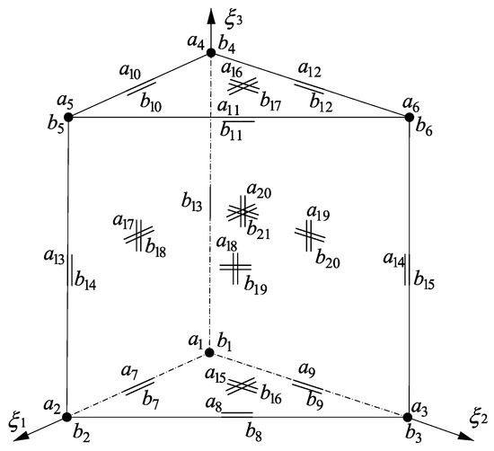
Figure 1.
An exemplary principal geometry I of the transition elements.
It is worth mentioning that the generalized (varying-order) nodes of both types may contain multiple degrees of freedom along the edges, within the bases and sides, and in the interior of the element. The related finite element approximations within the proposed element are all based on the general rules proposed by Demkowicz and others [1,2].
In the example of the second transition geometry II, shown in Figure 2, one deals with two vertical edges (nodes and ) and the side (nodes ) between these edges, all corresponding to the first-order mechanical model. The rest of the element (nodes ) conforms to the hierarchical shell model or the three-dimensional model of elasticity. These mechanical models are coupled with the symmetric-thickness hierarchical or three-dimensional models of dielectricity. The same nodes , as for the geometry I, are employed in this case.
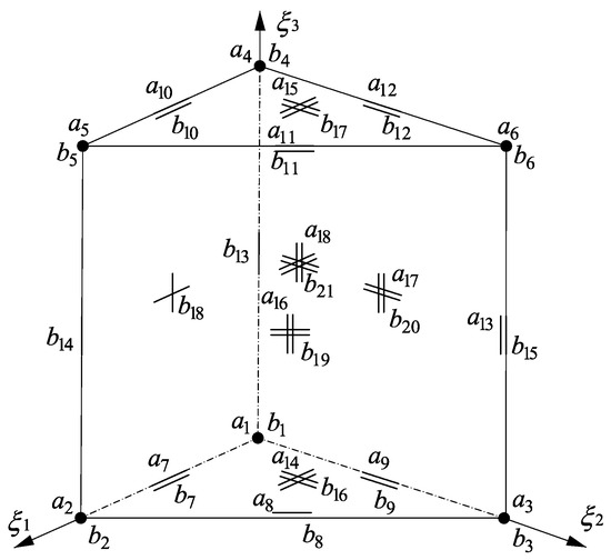
Figure 2.
An exemplary principal geometry II of the transition elements.
4.2. Element Characteristic Matrices and Vectors
Replacement of the global quantities introduced in (24) by the corresponding sums of the element (or local) quantities leads to
where e is the element number, while and stand for the element, displacements and potential, dofs vectors.
The element stiffness matrix is defined in the standard way, namely:
with relating strains with the element displacement dofs and, hence, named the element strain-displacement matrix. The matrix D represents the matrix of elasticities for the isotropy case under consideration, while the term is the determinant of the Jacobian matrix transforming the global coordinates x into normalized ones . Note that the applied normalized prismatic geometry of the element e can be characterized with . In the case of the thick- or thin-walled geometry, the first two normalized directions coincide with the longitudinal shell directions and the third normalized direction is the same as the transverse shell direction.
The definition of the element characteristic matrix of dielectricity reads
where allows expressing the electric field E with the element electric potential dofs . It is called the element field-potential matrix. The matrix is the constitutive constant matrix of orthotropic dielectricity under constant strain.
The element characteristic matrix of piezoelectricity coupling the mechanical and electric fields is defined as follows:
with C being the constitutive matrix of orthotropic piezoelectricity under constant strain.
The element nodal forces vector due to the mass loading f is defined in the standard way, i.e.,
with standing for the standard shape functions matrix corresponding to the vectorial displacement field.
In addition the element nodal forces due to the surface loading p is defined in the standard way, for the bases and lateral sides, respectively:
Above, , is identical to the directions of the triangle edges, i.e., either or or , while the coefficient transforms the surface element of the part of the domain surface S from the global coordinates to the normalized ones.
Finally, the element nodal charges due to the charge density c are equal to
for the element bases and sides, respectively, with denoting the standard shape function matrix suitable for the finite element approximation of the scalar electric potential field.
In the next subsection, we will present the changes that have to be implemented in the above finite element formulation depending on the applied transition model.
4.3. Strain-Displacement Matrix
Three cases of the classical, modified, and enhanced transition elements corresponding to the analogous transition models are of interest in this section.
4.3.1. The Transition Element Based on the Classical Model
The strain-displacement matrix for the classical transition model is assumed in the form corresponding to the three-dimensional elasticity and the hierarchical shell models, for the three-dimensional and thick- or thin-walled geometries, respectively. This means that the three-dimensional strain and stress state is applied for this classical model. This state is characterized by
and reflects the relation between the local strains and global nodal displacement dofs . The local strain directions are coincident with two tangent (the first two or two longitudinal) and one normal (the third or transverse) directions within the structure.
The strain-displacement matrix will also be denoted as in our further considerations. The form of this matrix is derived from the standard approach applied to five-parameter thick-shell elements of the second order [63]. Here, we adopt it to the needs of the 3D-based hierarchical shell model. This form reads:
The above blocks of the strain-displacement matrix correspond to the element displacement dofs at the element nodes and are composed of the following components:
Any term , , of each block , where m corresponds to each of six components of the strain vector and n to each global direction of the displacement dof vector, can be determined as equal to:
with the terms representing components of the transformation matrix which converts the local Cartesian directions of the displacement dofs into the global ones. The terms can be calculated from
where the quantities are the partial derivatives, with respect to the normalized directions , of the shape function from the corresponding shape function matrix. The auxiliary quantities are equal to:
with the terms representing terms of the inverse Jacobian matrix and being the components of the transposed transformation matrix . The latter matrix transforms derivatives with respect to the global Cartesian directions into derivatives with respect to the local Cartesian directions. The terms of the transformation matrices can be obtained from:
where the unit vectors components , , , can be obtained from the vectors U, V and W equal to:
where the partial derivatives , are the terms of the Jacobian matrix J.
4.3.2. The Modified and Enhanced Transition Elements
In the case of these two types of the transition element, the constitutive relations (29) and (30) hold within the coupled mechanical field. The strain and stress state changes from the three-dimensional one to the plane stress state. This can be expressed with the following relation
where the components and correspond to the three-dimensional and plane stress states. The first component is defined in accordance with (44)–(50). The second component is divided into blocks corresponding to the displacement dofs at the element nodes, namely
Due to the plane stress assumption (21), any block k of the second component needs the following modification:
where the terms , , are defined in accordance with (46)–(50).
Because of the modified definition (51) of the strain vector , also any block k of the strain-displacement matrix has to be modified in accordance with
The blending function is defined in accordance with , i.e., as a function of the two normalized directions, and , tangent to the mid-surface defined with . Note that, for and , the definition (54) transforms into (45) and (53), suitable for the basic (three-dimensional and first-order) piezoelectric elements, respectively.
4.4. Field-Potential Matrix
For any type of the transition models: (16), (23), (24), and (30) plus (32), the definition of the electric field vector E remains unchanged. Because of this also the field-potential matrix has the same form for the classical, modified, and enhanced transition elements. This form corresponds to the three-dimensional or hierarchical symmetric-thickness dielectric models. For these models, the following relation holds:
Above, the locally defined electric field E is expressed with the scalar potential dofs .
The form of the electric field-potential matrix under consideration is
where the blocks of the field-potential matrix correspond to the electric potential dofs of the element. The number of these blocks may be different to the number of the displacement dofs as the electric potential field is -interpolated, while the displacement field is -interpolated. The form of these blocks is:
The terms , where are the local Cartesian directions, are equal to
Note that the quantities , are the derivatives of the terms of the shape function matrix with respect to the normalized directions . The shape function corresponds to the electric potential dof l at the element node. The auxiliary terms , can be calculated from
i.e., analogously as in the case of the strain-displacement matrix. As before, the terms belong to the transformation matrix which transforms the local Cartesian directions into global Cartesian ones . The quantities are the terms of the inverse Jacobian matrix again.
4.5. Constitutive Constant Matrices
In the case of the classical, modified, and enhanced transition elements, the constitutive, elasticity constant matrix from (37) takes the same form (13).
The classical transition element requires the dielectricity and piezoelectricity constant matrices, in (38) and (39), in the form defined by (18) and (19), respectively. As far as the modified and enhanced transition elements are concerned, one has to apply, in relations (38) and (39), the definitions included in (32) and (30), respectively.
4.6. Blending Functions
As said above, blending functions describe the linear change of the stress state within transition elements from the three-dimensional to plane stress state. This change manifests itself by the presence of function in the strain definition of the modified and enhanced transition elements and in the piezoelectric and dielectric constant matrices for these two transition elements. Note that , are the normalized directions within an element and defines location of the reference surface within the element.
The blending function corresponding to the transition element of the geometry I is presented in Figure 3. The function is represented by the triangle spanned at the vertices , , and takes the value of 0 for the vertical edge 1 corresponding to the mechanical field of the first-order in the transverse direction and to the electric field of an arbitrary order in this direction. The blending function value of 1 corresponds to the mechanical and electric fields of arbitrary orders for the vertical edges 2 and 3. This function can be expressed with the affine coordinates , of the triangular element base or the normalized coordinates and as
where , and .
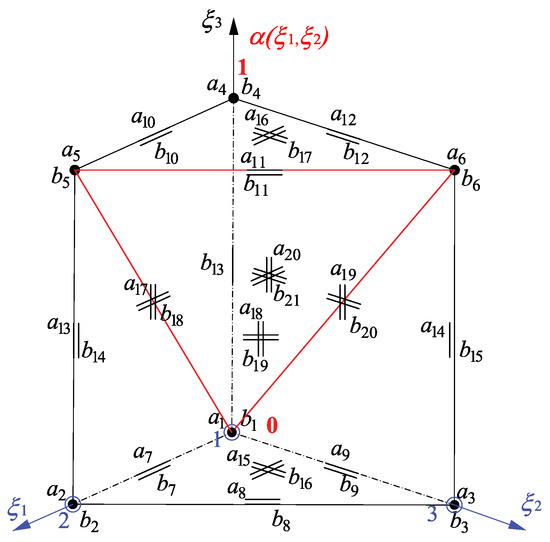
Figure 3.
The blending function for an example of the principal transition geometry I.
The geometry II of the transition element and the respective blending function are presented in Figure 4. The function is represented by the triangle spanned at the vertices , , and equals 0 for two edges 1 and 2 corresponding to the mechanical field of the first-order in the transverse direction. This value is equal to 1 for the vertical edge 3 where the mechanical field is of arbitrary order in the transverse direction . The order of the electric field is arbitrary for all three vertical edges. The function can be expressed in the following way:
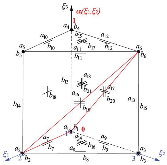
Figure 4.
The blending function for an example of the principal transition geometry II.
It should be noted that due to introduction of the linear blending functions into the vectors and matrices from (29)–(32), the polynomial order the integrands of (37)–(39) increases. This needs the respective increase of the number of the Gauss points in the numerical integration of these integrands.
4.7. Shape Function Matrices
The shape function matrices corresponding to the displacement field of the transition piezoelectric elements are of the standard form for any type of the element. This form reads
where the blocks are diagonal and correspond to the vectorial displacement dofs k at the element node:
In the case of the electric potential, the following standard form of the shape function matrix is valid for the piezoelectric transition element of any type:
where the blocks , corresponding to the scalar electric potential dof l at the element node, reduce to:
4.8. Kinematic Constraints within the Elements
In this section, the algorithms for imposition of the constraints of no elongation of the normals to the mid-surface, and for application of the constraints imposed on the generalized (varying-order) displacement dofs, as well, will be presented.
4.8.1. The Classical and Modified Elements
Stiffness Matrix Modification
In this case the constraints of no elongation of the normals are assumed on the boundary between the first-order and transition elements. These constraints are imposed with the penalty method where the parameter P is employed. It represents the inverse of the penalty parameter and is a number sufficiently large to overwrite the stiffness matrix terms with the constraint terms and to replace the finite element equation with the constraint equation. Our approach takes advantage of the presentation of the method given in Reference [1,2]. Imposition of the constraints under consideration needs the following modification of the stiffness matrix:
where is called the penalty matrix. Its terms include the mentioned parameter P.
Note that no modification of the force vectors due to penalty method is required as one deals with zero constraints in the paper, e.g., the constraints of no elongation of the normals to the mid-surface. The same refers to other constraints presented in this paper.
The arithmetic operator matrices and of the element e from (66) are capable of converting the top and bottom displacement dofs into their mean sums and differences, and conversely, respectively. The form of the first operator is related to the division of the element dofs into two groups: the pairs of top and bottom displacement dofs and all other displacement dofs , namely:
where the two blocks consist of the following component sub-blocks:
The top and bottom dofs, k and l, are associated with the nodes belonging to only. In the case of the transition element geometry I (Figure 3), the top dofs k are associated with the node , the bottom dofs l with the node , the other dofs m with the nodes . In the case of the geometry II, one has the following assignments: the top dofs k are associated with the nodes , the bottom dofs l with the nodes , the other dofs m with the nodes .
Modifying Operators
Following the above assignments, one defines
Within the block , the following overlapping sub-blocks can be distinguished
Sub-blocks , are responsible for summation of the top and bottom displacement dofs, while and for subtraction of these dofs. In turn, the block possesses the following structure based on the identity sub-blocks I
This means that neither the summation nor the subtraction is performed for the dofs m.
One more remark concerns the sums and differences of displacements present in the constraints (27). In the case of the symmetric-thickness geometry, these sums define mid-surface displacements. The first two differences, after division by the thickness t, give rotations of the normal to the mid-surface, while the third difference determines a transverse elongation of the corresponding normal. Note that only the latter difference needs to be constrained (equal to zero) in accordance with the last Equation (27). Because of this, multiplication of the penalty stiffness by the diagonal matrix Z is necessary. This matrix possesses the following structure:
The component block is composed of the diagonal blocks and corresponding to the degrees of freedom k and l:
where the degrees of freedom k and l correspond to the sums and differences of the top and bottom displacement dofs. The second component block has the simpler form
which results from the fact that, for the degrees of freedom m, other than the sums and differences of the displacement dofs, the penalty terms are not necessary.
Penalty Stiffness
The respective penalty stiffness , present in (66), is defined in the directions coincident with the constraint directions of which the first two are tangent and the third one is perpendicular to the mid-surface. The stiffness form corresponds to the displacement dofs that represent the mentioned sums and differences of the top and bottom dofs. The definition of the penalty stiffness reads:
The penalty parameter has to be larger than the terms of and the terms of , i.e., , where represent terms of the stiffness matrix and stands for the corresponding number of displacement dofs. Additionally, one has , with being terms of the piezoelectricity matrix and denoting the corresponding number of electric potential dofs.
The above form (75) of the penalty matrix is suitable for the geometry I of the classical and modified transition elements. In the above equation, stands for the element side being the subset of the boundary R between the first-order and transition model: . The normal vector n is defined as perpendicular to the mid-surface , i.e., . It also approximately satisfies the condition – approximately due to the finite element approximation of the element geometry. Note that two tangential directions and the third normal direction are coincident with the local directions present in the constraint Equation (27). On the element level, they are defined by the relations (49) and (50). Note also that the presence of the vector n in the above definition results in imposition of the penalty terms in the third (normal) direction only, i.e., the constraints are applied in this direction only. The shape function matrix terms are non-zero on the boundary . Hence, the non-zero penalty terms appear for the element nodes placed on this boundary.
In the case of the classical and modified transition elements of the geometry II, the above definition has to take into consideration the fact that the constraints (27) are imposed on the element vertical edge only. The edge can be characterized with: . The normal vector is defined analogously as in the case of the geometry I, i.e., and approximately . With these remarks in mind, one can write
where, due to one dimensional integration, the value of is applied for transformation of the global directions into the normalized direction . As previously, the constraints concern the differences of the top and bottom displacement dofs. The non-zero penalty terms appear for the element nodes and the corresponding dofs placed on the boundary , in the transverse direction only.
4.8.2. The Enhanced Transition Element
Two types of constraints are present in the case of the corresponding transition model. The first type are the gradually changing constraints of no elongation of the normals to the mid-surface, represented by the last but one term of (34). The considered type of the element requires also the additional constraints corresponding to the gradual change of the transverse order of approximation from to an arbitrary value , where I is the hierarchical model order, and represented by the last term of (34). As the constraints of both types are fully active on the boundary with the first-order model () and gradually switched off () towards the boundary with the hierarchical or three-dimensional model, the nodal (collocation) values of the complement of the switching functions to unity will appear in the penalty stiffness definitions so as to activate the penalty terms.
The Modified Stiffness Matrix
The relations (66)–(68) are still valid for the enhanced transition elements and constraints of no elongation of the normals to the mid-surface . However, the degrees of freedom k and l corresponding to the top and bottom displacements, and the other dofs m, as well, are associated with different nodes now because the constraints of no elongation of the lines normal to the mid-surface are applied in the entire element volume . In the case of the geometry I, the top dofs k are associated with the nodes the bottom dofs l with the nodes , and the other dofs m with the nodes . The geometry II needs the following assignments: the top dofs k correspond to the nodes , the bottom dofs l to the nodes , and the other dofs m to the nodes . These assignments hold also for the constraints related to the change of the transverse approximation order. In this case, the stiffness matrix modification is described with the relation
The Modifying Operators
In the case of the constraints of no elongation of the normals, the definitions of the operators and Z, (69)–(71) and (72)–(79), respectively, are still valid. However, the new assignments of the top k, bottom l, and other m dofs to the element nodes for geometries I and II have to be taken into account while calculating the corresponding operator matrices. In the case of the constraints of the second type, which concern the other dofs m only, the following definition is appropriate
As it can be seen, the first component block of (78) is . The second component block has the form
which results in appearance of the penalty terms for all dofs m in all three global directions.
The Penalty Matrices
The constraints of no elongation of the normals require the following definition of the penalty stiffness matrix:
where normal vector is , with being the mid-surface within the symmetric-thickness geometry. The presence of this vector results in application of the constraints in the normal direction only. In turn, the presence of the switching function guarantees the gradual change of the penalty terms. It employs the identity matrix I and the matrix of nodal values of the blending function:
and the nodal blocks are diagonal and correspond to the dofs m, other than the top and bottom ones:
and where . Its value depends on the longitudinal location of the node, the dof m is associated with. In other words, , where and represent first two normalized coordinates for the dof m.
In the case of the constraints of the second type one has
These constraints also change gradually and are applied in all three global directions for degrees of freedom m of the element. The definitions (81) and (82) of the switching function remain unchanged.
It should stressed that the above definitions (80) and (83) are valid for both the transition elements acting between the piezoelectric elements based on the first-order shell theory and the elements based on either the hierarchical shell theory or the three-dimensional theory. The difference is that, in the first case, the entire surface (characterized with ) represents the shell mid-surface, while, in the second case, it represents the reference surface only (defined with ). The reference surface becomes the mid-surface only on the boundary with the first-order model .
5. Numerical Tests
Two aspects of performance of the proposed transition piezoelectric elements will be addressed in this section. The first one is the ability to remove high stress gradients between the 3D-based transition and 3D-based basic elements in the chosen model problems. The mechanical models of the basic elements conform to the 3D-based first-order shell theory and the 3D-based hierarchical shell or three-dimensional theory. The electric field is characterized with the same dielectric model conforming to either three-dimensional or 3D-based hierarchical symmetric-thickness theory.
The second aspect will be comparison of the solution convergence for the same model problems as in the first aspect with three versions of the transition elements employed. The model problems will concern the bending-dominated plate and shell and membrane-dominated shell. These problems manifest different and numerically demanding stress and strain states. Explanation of the differences between these three cases of the mechanical fields can be found in Reference [53]. The electric field and electric displacement states will be typical for piezoelectricity.
It should be stressed that our model problems presented below serve the numerical assessment of the presented algorithms. Because of that the loads and charges are assumed so as the mechanical and electric parts of the potential electro-mechanical energy (or potential co-energy) are of the same order – the case very demanding from the numerical point of view as the sign of the electro-mechanical potential energy may change in the convergence studies where the error of the energy is displayed as a function of the number of dofs in the problem. Note that, in the two technologically important actuating and sensing modes of piezoelectric operation, one part of the co-energy dominates the other one. Because of this, such modes are less demanding numerically.
5.1. Model Problems and Methodology
5.1.1. Model Structures and Their Geometry
Three piezoelectric domains corresponding to the bending-dominated plate, bending-dominated half-cylindrical shell and a half of the membrane-dominated cylindrical shell are presented in Figure 5, Figure 6 and Figure 7. The plate dimensions are , the length of both shells is equal to l, while the circumferential length of a half of the cylinder is with R being the radius of the mid-surface of the shells. All the structures are of the same thickness t. The following values are set in our tests: m, m, m.
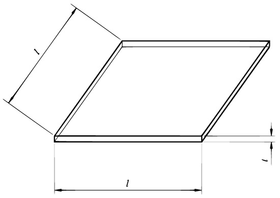
Figure 5.
The domain of the bending-dominated piezoelectric plate.
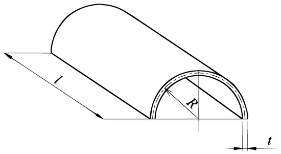
Figure 6.
The domain of the bending-dominated piezoelectric half-cylindrical shell.
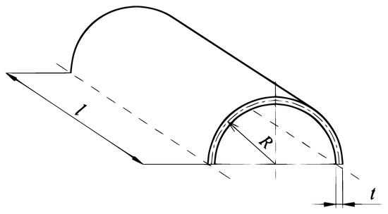
Figure 7.
A half of the membrane-dominated piezoelectric shell domain.
5.1.2. Material, Load, Charge and Boundary Conditions
All three structures are made of the same piezoelectric material of material constants typical for piezoceramics [57]. The Young modulus is , the Poisson ratio equals , the dielectricity constant under constant stress is F/m, while the piezoelectric constants under constant stress are equal to C/N, C/N, and C/N.
The plate and bending-dominated shell are loaded with the vertical traction of the value , while the membrane-dominated shell with the internal pressure of the same value p acting in the outward direction. All the structures are electrically charged on their upper (or outward) surface where the surface charge density is . On the lower (or inward) surfaces the charge density is set to 0.
The mechanical boundary conditions are as follows. The plate is clamped along its four edges. The bending-dominated shell has two straight edges clamped and two curved edges free. In the case of the membrane-dominated shell, there is no rotation along the curved edges. The electrical boundary conditions assume grounding along: four edges of the plate, along two straight and two curved edges of the half-cylindrical shell, and two curved edges of the cylindrical shell.
5.1.3. Discretization and Methodology
Due to symmetry of the geometry, loading, electric charge, and boundary conditions, only quarters of the bending-dominated domains and an octant of the membrane-dominated domain are taken into account in or numerical tests and presented in the figures below. The numerical settings are as follows. We apply the meshes of the prismatic elements in the displayed quarter or octant parts of the structures in our tests. The longitudinal order of approximation within the mechanical and electric field is the same and equal . The transverse orders of approximation of both fields are equal to in the hierarchical shell zone of the domains, in the first-order shell zone, and the changing (from 2 to 1) order in the transition zone constituting a layer composed of couples of prismatic transition elements. The number of the first-order and hierarchical (three-dimensional) elements changes from the entirely hierarchical shell structure to the shell structure composed of the first-order shell elements only. The intermediate (or mixed) case includes a single layer of piezoelectric transition elements. The exemplary cases for the plate and shells are presented in Figure 8, Figure 9 and Figure 10.
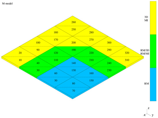
Figure 8.
Mixed models of the bending-dominated plate.
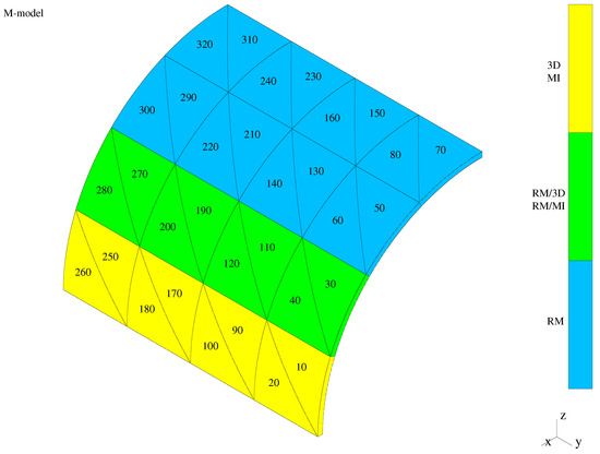
Figure 9.
Mixed models of the bending-dominated shell.
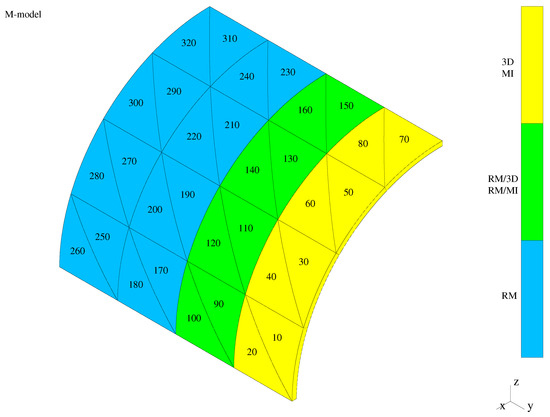
Figure 10.
Mixed models of the membrane-dominated shell.
The presented meshes are composed of one layer of hierarchical elements (yellow and marked as MI in the figure), one layer of the transition elements (green and marked as RM/MI), and two layers of the first-order elements (blue and marked as RM in the figure).
Our parametric studies are limited to changes of the longitudinal approximation orders , the ratios of the numbers of elements of various types, and the types of the transition elements for three model problems. The mentioned ratios are equal to and represent the number of the first-order elements divided by the sum of the transition and hierarchical elements along the characteristic longitudinal dimensions of the structures.
5.2. Ability to Remove High Stress Gradients
In order to present the ability of three (classical, modified, and enhanced) types of the transition elements to remove the high stress gradients between the transition elements and the neighboring basic (hierarchical and first-order) elements, exemplary () distributions of the global normal stress (marked as ) for three model problems and three types of the transition elements are presented. These distributions correspond to the mixed models from Figure 8, Figure 9 and Figure 10. The stress distributions for the plate problem, with the classical, modified and transition elements employed, are presented in Figure 11, Figure 12 and Figure 13, respectively. Figure 14, Figure 15 and Figure 16 display the analogous three stress distributions for the bending-dominated shell. The last figures, Figure 17, Figure 18 and Figure 19, correspond to the membrane-dominated problem with three types of the transition elements applied. Note that, in the figures, the stress values are written in numerical form not in analytical form due to capabilities of the numerical code used.
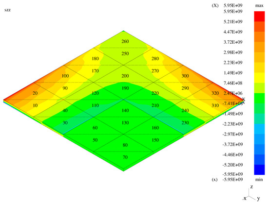
Figure 11.
Transverse stress—the bent plate with the classical transition elements.

Figure 12.
Transverse stress—the bent plate with the modified transition elements.

Figure 13.
Transverse stress—the bent plate with the enhanced transition elements.

Figure 14.
Third normal stress—the bent shell with the classical transition elements.

Figure 15.
Third normal stress—the bent shell with the modified transition elements.
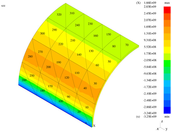
Figure 16.
Third normal stress—the bent shell with the enhanced transition elements.
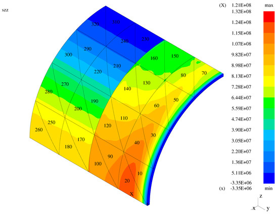
Figure 17.
Third normal stress—the membrane with the classical transition elements.

Figure 18.
Third normal stress—the membrane with the modified transition elements.
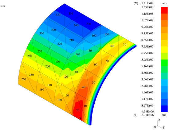
Figure 19.
Third normal stress—the membrane with the enhanced transition elements.
In the case of the plate and membrane problems, high solution gradients are visible when the classical transition elements are employed. These gradients are reduced for the mixed models with the modified and enhanced elements applied. In the case of the bent shell, high gradients are not visible for the classical elements as the displayed global normal stress component is a combination of the transverse and longitudinal stresses.
In order to quantify the presented graphical results concerning stress gradients, the Table 1 is presented. Therein, gradients (jumps/differences) of the global stress between the face centers of the neighboring elements are displayed for three model structures. Five models for each of three structures are included: the entirely hierarchical (MI) shell model (), three mixed (RM/MI) models () with the classical, modified, and enhanced (respectively, TR1, TR2, TR3) transition models, and entirely first-order (RM) model (). In the case of the bending-dominated (bent) plate, the chosen elements 31 and 24 correspond to 3D model and TR1 or TR2 or TR3 model. Both elements 24 and 23 correspond to either TR1 or TR2 or TR3 model, while the elements 23 and 16 to either TR1 or TR2 or TR3 model and RM model. In the case of the bending-dominated (bent) shell, the corresponding couples of elements are: 25 and 28, 28 and 27, and 27 and 30. In the case of the membrane (membrane-dominated shell), the corresponding couples are: 6 and 13, 13 and 14, 14 and 21.

Table 1.
Summary of stress gradients [N/m] for three model problems.
In the case of the plate, the third normal stress corresponds to the transverse normal stress. In the entirely hierarchical (MI) shell model, the observed values of gradients are small and due to finite element discretization. In the entirely first-order (RM) model, the jumps are extremely small (correspond to the numerical zero), as the plane stress assumption holds in all elements. In the case of the mixed TR1 model, the jump between the transition and first-order elements 23 and 16 results from the three-dimensional stress state and plane stress state in the neighboring elements. Such jumps are diminished to numerical zero for the cases of the TR2 and TR3 models, as the plane stress assumption holds on both sides of the neighboring faces of the transition and first-order elements. In both shell cases, the presented jumps of result from both discretization and plane stress assumption. The exact analysis for the transverse direction requires taking jumps for the stress components and into account. Such an analysis (not revealed here) leads to exactly the same observations as in the case of the plate. For the membrane case, where the contribution of to the transverse normal stress is higher than the influence of two other stress components, the stress jumps in between elements 14 and 21 are smaller in the case of the TR3 model than in the cases of the TR2 and TR1 models. In the bent shell case, the jumps in between elements 27 and 30 grow from TR1 through TR2 to TR3, but this leads to zero transverse normal stress values in both neighboring elements for the TR2 and TR3 models. Demonstration of this needs inclusion of the stress components and again.
5.3. Solution Convergence of the Problems
In the convergence studies, the logarithm of the approximation error in potential energy is presented as a function of the logarithm of the number of dofs N of the problem. The corresponding curves are p-convergence ones as the number of dofs in the problems increase due to the change of the longitudinal order of approximation p within elements. In order to present the solution convergence for the three model problems with three types of the transition elements applied, three threesomes of pictures are displayed. The first three pictures (Figure 20, Figure 21 and Figure 22) correspond to the bending-dominated plate problem, the second threesome (Figure 23, Figure 24 and Figure 25) to the bending-dominated shell problem, while the last three drawings (Figure 26, Figure 27 and Figure 28) to the membrane-dominated shell. In the figures, the first, second and third drawings correspond to the cases of the classical, modified, and enhanced transition elements applied.
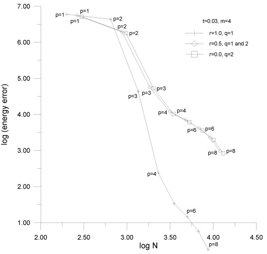
Figure 20.
Convergence curves—the plate problem, the classical transition elements employed.
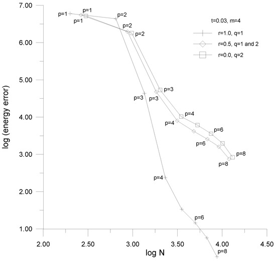
Figure 21.
Convergence curves—the plate problem, the modified transition elements applied.
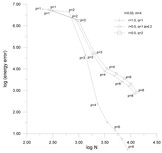
Figure 22.
Convergence curves—the plate problem, the enhanced transition elements applied.
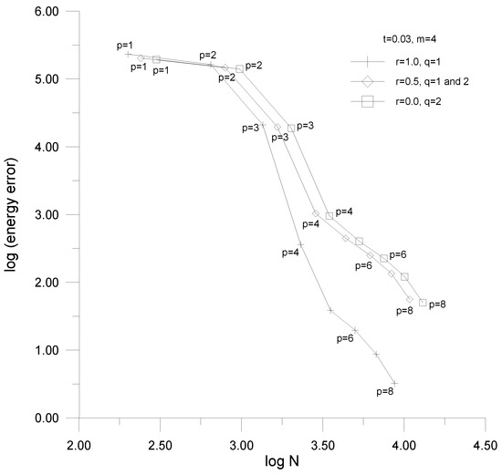
Figure 23.
Convergence curves—the bending-dominated shell with the classical transition elements.
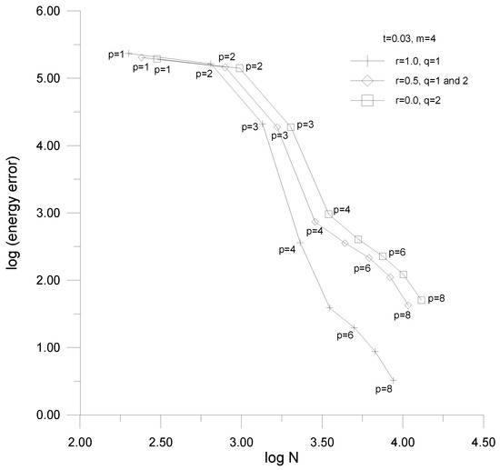
Figure 24.
Convergence curves—the bending-dominated shell with the modified transition elements.
Figure 25.
Convergence curves—the bending-dominated shell with the enhanced transition elements.
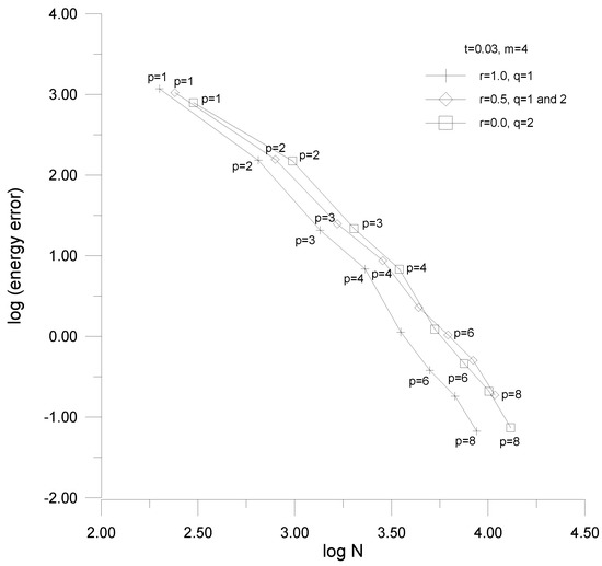
Figure 26.
Convergence curves—the membrane shell with the classical transition elements.
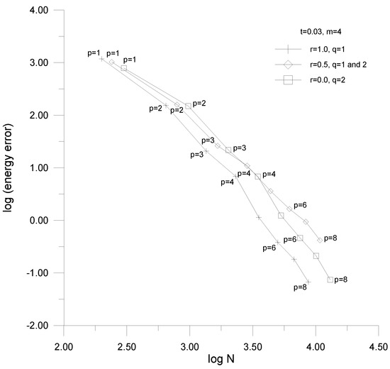
Figure 27.
Convergence curves—the membrane shell with the modified transition elements.
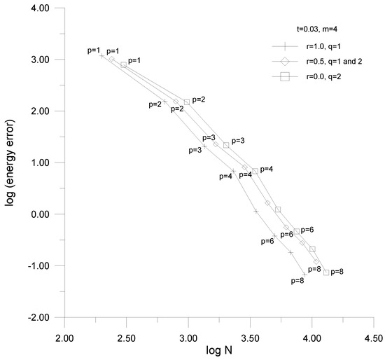
Figure 28.
Convergence curves—the membrane shell with the enhanced transition elements.
The mentioned approximation error is defined as the difference of two energy measures of which E corresponds to the numerical solution under consideration and the reference solution plays a role of the exact solution, namely:
The energy measures represent the sum of absolute values of the mechanical and electrical parts of the electro-mechanical potential energy, i.e.,
Due to stationarity of the solutions u and , resulting from (8), the potential energy can be expressed with the components of the electro-mechanical co-energy (strain, electric field, and coupling energies) corresponding to the bilinear forms B, b and C from (9)–(11). The solutions for displacements u and electric potential are approximated with use of the global nodal vectors of the displacement dofs and potential dofs obtained from solution of the problem (35).
The proposed measure of the approximation error was applied as it guarantees monotonicity of the energy approximation error with changing value of , while the simple sum of both parts of the energy (equal to the electro-mechanical co-energy) may not. Note that such monotonicity is a must in the case of error-controlled adaptivity suggested in Reference [11,12].
In order to calculate the errors, the exact values of the energy measures are replaced with their best numerical approximations obtained from the so-called over-killed meshes, i.e., the meshes for which the longitudinal order of approximation is equal to .
In the case of two bending-dominated problems the convergence for the enhanced models is slightly higher than for the modified transition elements employed in the mixed models. Additionally, the latter elements produce slightly better convergence than the classical ones. In the case of the membrane-dominated problem, only the enhanced transition elements deliver convergence curves between the curves obtained for the basic models. The confirmation is presented in the Table 2, where the absolute values log of the error and relative error values (both for , i.e., ) are included. In addition, the averaged convergence rates are given and equal to −loglog, , , where , and , represent the energies and numbers of dofs for and .
Table 2.
Error and convergence summary for three model problems.
6. Conclusions
Three types of the transition piezoelectric elements joining the basic piezoelectric elements are possible. The joined basic elements are the three-dimensional piezoelectric elements (or hierarchical symmetric-thickness piezoelectric elements) and the first-order symmetric-thickness piezoelectric elements.
The first (classical) transition element guarantees continuity of the displacement and electric potential fields between the basic elements. It also guarantees that the assumption of no elongation of the normals to the mid-surface holds on the boundary between the transition elements and the first-order elements.
The second (modified) transition element, additionally, guarantees the gradual change from the plane stress to three-dimensional stress state between the basic elements of the first-order and three-dimensional (or hierarchical) character, respectively.
The third (enhanced) transition element, additionally, assures the gradual change of the assumption of no elongation of the normals to the mid-surface between the basic elements. The latter assumption holds on the boundary with the first-order element and is gradually switched off towards the boundary with the three-dimensional (or hierarchical) element. On this boundary, this assumption is completely off.
The gradual change of the stress state from the plane to three-dimensional is based on introduction of the blending functions that determine contributions of the basic models to the transition model. Implementation of this idea on the element level needs modifications of the strain vector, and the piezoelectric and dielectric constant matrices as well.
The gradual change of the assumption of no elongation of the normals needs utilization of the blending functions, which play the role of gradually switching functions. On the element level, the nodal values of the complement (to unity) of the gradually switching functions appear in the penalty stiffness matrix responsible for the gradual change of the constraints.
Comparing the stress distributions within the transition zones for three model problems, one can notice that high stress gradients appear on the boundary between the classical transition elements and the first-order elements. In the case of the enhanced transition elements, the gradual change of the stress state can be observed. In the case of the modified transition element, the stress distribution is intermediate with respect to the previous two distributions.
It can be observed that the discrete models of the three analyzed model structures, with three types of the transition elements employed, produce the convergence curves of slightly higher convergence for the case of the modified elements in comparison to the classical elements. The highest convergence, however, is obtained in the case of the enhanced transition elements.
It can be concluded that the enhanced transition element should be recommended in the analysis of mixed models of piezoelectrics, as this element gives the same or better convergence than the other transition models, and it removes the high stress gradients between the classical transition elements and the first-order piezoelectric elements.
Even though all three transition models can be applied to error-controlled adaptivity due to monotonicity of the applied error measure, the enhanced transition elements deliver convergence curves with the error level and convergence rates just between the curves for the basic models.
The presented research needs the following next steps. Firstly, the error estimation methods and adaptive procedures for the new transition elements have to be prepared and verified. Next, application of the proposed transition models to parametric and/or adaptive analysis of electro-mechanical systems should be performed and critical factors influencing quality of such an analysis should be determined.
Author Contributions
Conceptualization, G.Z. and M.Z.; methodology, G.Z. and M.Z.; writing and verifying software, G.Z. and M.Z.; validation, G.Z. and M.Z.; formal analysis, G.Z. and M.Z.; investigation, G.Z. and M.Z.; resources, G.Z. and M.Z.; writing—original draft preparation, G.Z. and M.Z.; writing—review and editing, G.Z. and M.Z.; projects administration, G.Z. and M.Z.; funding acquisition, G.Z. and M.Z. Both authors have read and agreed to the published version of the manuscript.
Funding
This research was partly funded by Scientific Research Committee Poland under research grants 7 T07A 004 14 and 5 T07A 040 24 and by National Science Center Poland under research grant N N504 515340.
Institutional Review Board Statement
Not applicable.
Informed Consent Statement
Not applicable.
Conflicts of Interest
The authors declare no conflict of interest.
References
- Demkowicz, L. Computing with hp-Adaptive Finite Elements. Vol. 1. One- and Two-Dimensional Elliptic and Maxwell Problems; Chapman & Hall/CRC: Boca Raton, FL, USA, 2007. [Google Scholar]
- Demkowicz, L.; Kurtz, J.; Pardo, D.; Paszyński, M.; Rachowicz, W.; Zdunek, A. Computing with hp-Adaptive Finite Elements. Vol. 2. Three-Dimensional Elliptic and Maxwell Problems with Applications; Chapman & Hall/CRC: Boca Raton, FL, USA, 2008. [Google Scholar]
- Auricchio, F.; Bisegna, P.; Lovadina, C. Finite element approximation of piezoelectric plates. Int. J. Numer. Meth. Eng. 2001, 50, 1469–1499. [Google Scholar] [CrossRef]
- Bisegna, P.; Maceri, F. A consistent theory of thin piezoelectric plates. J. Intell. Mater. Syst. Struct. 1996, 7, 372–389. [Google Scholar] [CrossRef]
- Lammering, R.; Yang, F. A Four-node Finite Element for Piezoelectric Shell Structures in Convective Co-ordinates. Proc. Appl. Math. Mech. 2006, 6, 237–238. [Google Scholar] [CrossRef]
- Lammering, R.; Mesecke-Rischmann, S. Multi-field variational formulations and related finite elements for piezoelectric shells. Smart Mater. Struct. 2003, 12, 904–913. [Google Scholar] [CrossRef]
- Braess, D.; Kaltenbacher, M. Efficient 3D-Finite-Element-Formulation for Thin Mechanical and Piezoelectric Structures. Int. J. Numer. Meth. Eng. 2008, 73, 147–161. [Google Scholar] [CrossRef]
- Botta, F.; Cerri, G. Wave propagation in Reissner-Mindlin piezoelectric coupled cylinder with non-constant electric field through the thickness. Solids Struct. 2007, 44, 6201–6219. [Google Scholar] [CrossRef]
- Madureira, A.L. Hierarchical modeling of piezoelectric plates. Appl. Math. Model. 2012, 36, 3555–3569. [Google Scholar] [CrossRef]
- Carrera, E.; Boscolo, M.; Robaldo, A. Hierarchic multilayered plate elements for coupled multifield problems of piezoelectric adaptive structures: Formulation and numerical assessment. Arch. Comput. Methods Eng. 2007, 14, 384–430. [Google Scholar] [CrossRef]
- Zboiński, G. Problems of Hierarchical Modelling and hp-Adaptive Finite Element Analysis in Elasticity, Dielectricity and Piezoelectricity. In Perusal of the Finite Element Method; Petrova, R., Ed.; InTech: Rijeka, Croatia, 2016; Chapter 1; pp. 1–29. [Google Scholar]
- Zboiński, G. Adaptive modeling and simulation of elastic, dielectric and piezoelectric problems. In Finite Element Method—Simulation, Numerical Analysis and Solution Techniques; Pacurar, R., Ed.; InTech: Rijeka, Croatia, 2018; Chapter 7; pp. 157–192. [Google Scholar]
- Zboiński, G. Hierarchical modeling and Finite Element Approximation for Adaptive Analysis of Complex Structures. D.Sc. Thesis, Institute of Fluid Flow Machinery, Gdańsk, Poland, 2001. (In Polish). [Google Scholar]
- Zboiński, G. Adaptive hpq finite element methods for the analysis of 3D-based models of complex structures. Part 1. Hierarchical modeling and approximation. Comput. Methods Appl. Mech. Eng. 2010, 199, 2913–2940. [Google Scholar] [CrossRef]
- Zboiński, G. Hierarchical models for adaptive modelling and analysis of coupled electro-mechanical systems. In Recent Advances in Computational Mechanics; Łodygowski, T., Rakowski, J., Litewka, P., Eds.; CRC Press: London, UK, 2014; pp. 334–339. [Google Scholar]
- Zboiński, G. 3D-based hierarchical models and hpq-approximations for adaptive finite element method of Laplace problems as exemplified by linear dielectricity. Comput. Math. Appl. 2019, 78, 2468–2511. [Google Scholar] [CrossRef]
- Krommer, M.; Irschik, H. A Reissner-Mindlin-type plate theory including the direct piezoelectric and the pyroelectric effect. Acta Mech. 2000, 141, 51–69. [Google Scholar] [CrossRef]
- Kant, T.; Shiyekar, S.M. Cylindrical bending of piezoelectric laminates with a higher order shear and normal deformation theory. Comput. Struct. 2008, 86, 1594–1603. [Google Scholar] [CrossRef]
- Bisegna, P.; Caruso, G.; Maceri, F. A layer-wise Reissner-Mindlin-type model for the vibration analysis and suppression of piezoactuated plates. Comput. Struct. 2001, 79, 2309–2319. [Google Scholar] [CrossRef]
- Kanber, B.; Bozkurt, O.Y. Finite element analysis of elasto-plastic plate bending problems using transition rectangular plate elements. Acta Mech. Sin. 2006, 22, 355–365. [Google Scholar] [CrossRef]
- Liao, L.; Yu, W. An electromechanical Reissner-Mindlin model for laminated piezoelectric plates. Compos. Struct. 2009, 88, 394–402. [Google Scholar] [CrossRef]
- Quoc, T.H.; Tham, V.V.; Tu, T.M. Active vibration control of a piezoelectric functionally graded carbon nanotube-reinforced spherical shell panel. Acta Mech. 2021, 232, 1005–1023. [Google Scholar]
- Kapuria, S.; Ahmad, A. A coupled efficient layerwise finite element model for free vibration analysis of smart piezo-bonded laminated shells featuring delaminations and transducer debonding. Int. J. Mech. Sci. 2021, 194, 106195. [Google Scholar] [CrossRef]
- Zielińska, M. Elastic Structures Analysis by the Adaptive Finite Element Method with Use of the Solid-to-Shell Transition Elements. Ph.D. Thesis, Faculty of Technical Sciences, University of Warmia and Mazury, Olsztyn, Poland, 2016. (In Polish). [Google Scholar]
- Surana, K.S. Transition finite elements for three-dimensional stress analysis. Int. J. Numer. Meth. Eng. 1980, 15, 991–1020. [Google Scholar] [CrossRef]
- Ahmad, S. Curved Finite Elements in the Analysis of Solid, Shell and Plate Structures. Ph.D. Thesis, University College of Swansea, Swansea, UK, 1969. [Google Scholar]
- Surana, K.S. Lumped Mass Matrices with Non-Zero Interia for General Shell and Axi-Symmetric Shell Elements. Int. J. Numer. Meth. Eng. 1978, 12, 1635–1650. [Google Scholar] [CrossRef]
- Surana, K.S. Geometrically nonlinear formulation for the axi-symmetric transition finite element. Comput. Struct. 1983, 17, 243–255. [Google Scholar] [CrossRef]
- Surana, K.S. Geometrically non-linear formulation for the three dimensional solid-shell transition finite elements. Comput. Struct. 1982, 15, 549–566. [Google Scholar] [CrossRef]
- Surana, K.S. Three dimensional solid-shell transition finite elements for heat conduction. Comput. Struct. 1987, 26, 941–950. [Google Scholar] [CrossRef]
- Bathe, K.J.; Bolourchi, S. A geometric and material nonlinear plate and shell element. Comput. Struct. 1980, 11, 23–48. [Google Scholar] [CrossRef]
- Gmür, T.C.; Schorderet, A.M. A set of three-dimensional solid to shell transition elements for structural dynamics. Comput. Struct. 1993, 46, 583–591. [Google Scholar] [CrossRef]
- Liao, C.L.; Reddy, J.N.; Engelstad, S.P. A solid-shell transition element for geometrically nonlinear analysis of laminated composite structures. Int. J. Number. Meth. Eng. 1988, 26, 1843–1854. [Google Scholar] [CrossRef]
- Cofer, W.F.; Will, K.M. A three-dimensional, shell-solid transition element for general nonlinear analysis. Comput. Struct. 1991, 38, 449–462. [Google Scholar] [CrossRef]
- Dávila, C.G. Solid-to-shell transition elements for the computation of interlaminar stresses. Comput. Syst. Eng. 1994, 5, 193–202. [Google Scholar] [CrossRef]
- Gong, Y. Local/global structural analysis by transition elements. Comput. Struct. 1988, 30, 831–836. [Google Scholar]
- Stein, E.; Rüter, M. Error-cotrolled adaptive modelling and finite element analysis in the context of European structural codes. In International Conference on Adaptive Modeling and Simulation ADMOS 2003; Wiberg, N.-E., Diez, P., Eds.; CIMNE: Barcelona, Spain, 2003; CD-Rom 1-28. [Google Scholar]
- Stein, E.; Ohnimus, S. Equilibrium method for postprocessing and error estimation in the finite element method. Comput. Assist. Mech. Eng. Sci. 1997, 4, 645–666. [Google Scholar]
- Niekamp, R.; Stein, E. An object-oriented approach for parallel two- and three-dimensional adaptive finite element computations. Comput. Struct. 2002, 80, 317–328. [Google Scholar] [CrossRef]
- Gupta, A.K. A finite element for transition from a fine to a coarse grid. Int. J. Numer. Meth. Eng. 1978, 12, 35–45. [Google Scholar] [CrossRef]
- Huang, F.; Xie, X. A modified nonconforming 5-node quadrilateral transition finite element. Adv. Appl. Math. Mech. 2011, 2, 784–797. [Google Scholar]
- Wan, K. Transition Finite Elements for Mesh Refinement in Plane and Plate Bending Analyses. Master’s Thesis, Mechanical Engineering Department, The University of Hong Kong, Hong Kong, China, 2004. [Google Scholar]
- Jeyachandrabose, C.; Kirkhope, J. Construction of transition finite elements for the plane triangular family. Comput. Struct. 1984, 18, 1127–1134. [Google Scholar] [CrossRef]
- Lo, S.H.; Wu, D.; Sze, K.Y. Adaptive meshing and analysis using transitional quadriateral and hexahedral elements. Finite Elem. Anal. Des. 2010, 46, 2–16. [Google Scholar] [CrossRef]
- Guzelbey, I.H.; Kanber, B. A practical rule for the derivation of transition finite elements. Int. J. Numer. Meth. Eng. 2000, 47, 1029–1056. [Google Scholar] [CrossRef]
- Kim, H.-S.; Hong, S.-M. Formulation of transition elements for the analysis of coupled wall structures. Comput. Struct. 1995, 57, 333–344. [Google Scholar] [CrossRef]
- Lim, J.-K.; Song, T.-H.; Seog, B.-H. Formulation Method for Solid-to-Beam Transition Finite Elements. KSME Int. J. 2001, 15, 1499–1506. [Google Scholar] [CrossRef]
- Garusi, E.; Tralli, A. A hybrid stress-assumed transition element for solid-to-beam and plate-to-beam connections. Comput. Struct. 2002, 80, 105–115. [Google Scholar] [CrossRef]
- Stein, E.; Rüter, M.; Ohnimus, S. Adaptive finite element analysis and modelling of solids and structures. Findings, problems and trends. Int. J. Numer. Meth. Eng. 2004, 60, 103–138. [Google Scholar] [CrossRef]
- Hauptmann, R.; Schweizerhof, K. A systematic development of solid-shell element formulations for linear and non-linear analyses employing only displacement degrees of freedom. Int. J. Numer. Meth. Eng. 1998, 42, 49–69. [Google Scholar] [CrossRef]
- Zboiński, G.; Ostachowicz, W. An algorithm of a family of 3D-based solid-to-shell transition hpq/hp-adaptive finite elements. J. Theor. Appl. Mech. 2000, 38, 791–806. [Google Scholar]
- Zielińska, M.; Zboiński, G. hp-Adaptive finite element analysis of thin-walled structures with use of the shell-to-shell transition elements. In Recent Advances in Computational Mechanics; Łodygowski, T., Rakowski, J., Litewka, P., Eds.; CRC Press: London, UK, 2014; pp. 63–72. [Google Scholar]
- Zboiński, G. Application of the three-dimensional triangular-prism hpq adaptive finite element to plate and shell analysis. Comput. Struct. 1997, 65, 497–514. [Google Scholar] [CrossRef]
- Zboiński, G.; Jasiński, M. 3D-based hp-adaptive first order shell finite element for modeling and analysis of complex structures—Part 1. The model and the approximation. Int. J. Numer. Meth. Eng. 2007, 70, 1513–1545. [Google Scholar] [CrossRef]
- Szabó, B.A.; Sahrmann, G.J. Hierarchic plate and shell models based on p-extension. Int. J. Numer. Meth. Eng. 1988, 26, 1855–1881. [Google Scholar] [CrossRef]
- Oden, J.T.; Cho, J.R. Adaptive hpq finite element methods of hierarchical models for plate- and shell-like structures. Comput. Methods Appl. Mech. Eng. 1996, 136, 317–345. [Google Scholar] [CrossRef]
- Premount, A. Mechatronics. Dynamics of Electromechanical and Piezoelectric Systems; Springer: Dordrecht, The Netherlands, 2006. [Google Scholar]
- Zboiński, G. Analytical aspects of the 3D-based hierarchical models of three-dimensional, transition and symmetric-thickness piezoelectrics as applied in adaptive FEM. In Shell Structures. Theory and Applications, Volume 4; Pietraszkiewicz, W., Witkowski, W., Eds.; CRC Press: London, UK, 2017; pp. 304–306. [Google Scholar]
- Ieşan, D. Reciprocity, uniqueness and minimum principles in the linear theory of piezoelectricity. Int. J. Eng. Sci. 1990, 28, 1139–1149. [Google Scholar] [CrossRef]
- Cimatti, G. The piezoelectric continuum. Ann. Metematica Pura Appl. 2004, 183, 495–514. [Google Scholar] [CrossRef]
- Babuška, I. Error-bounds for finite element method. Numer. Math. 1971, 16, 322–333. [Google Scholar] [CrossRef]
- Lax, P.D.; Milgram, A.N. Parabolic equations. In Contributions to the Theory of Partial Differential Equations, Annalsof Mathematics Studies 33; Princeton University Press: Princeton, NJ, USA, 1954; pp. 167–190. [Google Scholar]
- Hinton, E.; Owen, D.R.J. Finite Element Software for Plates and Shells; Pineridge Press: Swansea, UK, 1984. [Google Scholar]
Publisher’s Note: MDPI stays neutral with regard to jurisdictional claims in published maps and institutional affiliations. |
© 2021 by the authors. Licensee MDPI, Basel, Switzerland. This article is an open access article distributed under the terms and conditions of the Creative Commons Attribution (CC BY) license (https://creativecommons.org/licenses/by/4.0/).