Many-Objective Optimization for Anomaly Detection on Multi-Layer Complex Interaction Networks

Abstract

Anomaly detection in complex networks is an important and challenging task in many application domains. Examples include analysis and sensemaking in human interactions, e.g., in (social) interaction networks, as well as the analysis of the behavior of complex technical and cyber-physical systems such as suspicious transactions/behavior in financial or routing networks; here, behavior and/or interactions typically also occur on different levels and layers. In this paper, we focus on detecting anomalies in such complex networks. In particular, we focus on multi-layer complex networks, where we consider the problem of finding sets of anomalous nodes for group anomaly detection. Our presented method is based on centrality-based many-objective optimization on multi-layer networks. Starting from the Pareto Front obtained via many-objective optimization, we rank anomaly candidates using the centrality information on all layers. This ranking is formalized via a scoring function, which estimates relative deviations of the node centralities, considering the density of the network and its respective layers. In a human-centered approach, anomalous sets of nodes can then be identified. A key feature of this approach is its interpretability and explainability, since we can directly assess anomalous nodes in the context of the network topology. We evaluate the proposed method using different datasets, including both synthetic as well as real-world network data. Our results demonstrate the efficacy of the presented approach.

1. Introduction

With the current trends and advances in the digital transformation, an ever-increasing amount of complex relational data is observed. Naturally, such data and information can be modeled in networks; this specifically extends to multi-layer networks [1,2,3,4], which allow for modeling complex relationships on multiple levels or layers. Identifying and detecting anomalies in such complex networks is an important research problem that is relevant in various contexts, e.g., for the extended (behavioral) analysis of social interaction networks [5,6]. Further applications concern the analysis of (financial) transaction networks, cyber-physical systems, or trade networks. Here, the respective interactions can be analyzed, e.g., for detecting new knowledge about deviating (social/economical) behavior [7,8]. Specifically, the identification and analysis of sets of anomalous nodes is of particular interest, relating to the group anomaly detection problem. A further aspect is given by human-centered approaches, enabling computational sensemaking on the complex data and the detected anomalies, respectively.

In this paper—a substantially adapted and extended revision of [9]—we aim to identify and analyze potential anomalies in complex networks using many-objective optimization. We specifically focus on a specific class of networks, i.e., multiplex/multi-layer networks [2,10]. For multi-layer networks, each node is not only part of a single (layered) network but also part of multiple layers of a complex network. Here, a low/high centrality of a node in one layer of the network might not imply a low/high node centrality in another layer of the network. Multiplex networks are a special case of multilayer ones, being restricted to the same set of nodes in the layers and having according connections between layers [2]. Compared to our work in [9], we have both adapted/extended the presentation, the related work, the contextualization and description of the method, the discussion of the human-centered anomaly detection process, as well as the experimentation: Specifically, we present and discuss new experiments on three additional real-world datasets in our results and discussion.

In general, optimizing more than three objective function simultaneously can be categorized as many-objective optimization, yielding the Pareto Front in the multi-layer space. It is easy to see that different layers as different objective functions can be complementary. This means that, for example, minimizing the centrality of one layer could also imply minimizing the centrality of another layer as well. In contrast, the layers could also be contrary (conflicting) to the others. This then means that the structure of centrality is very different among the layers. Thus, our proposed method first estimates the centrality of all nodes in each layer of the multi-layer network, by applying many-objective optimization with full enumeration based on minimization and obtains the Pareto Front. The objective functions to be optimized simultaneously are the centralities of each layer in the network; thus, the number of objective function are given by the number of existing layers of a multi-layer network. Given the Pareto Front, we consider the contained set of nodes as a basis for identifying a candidate set of suspected anomaly nodes. For this, we apply the proposed novel ACE score for ranking the nodes. The ACE score is estimated using the centrality of the nodes relative to each layer, also taking the density of those layers into account. A high ACE score then indicates candidate anomalous nodes.

We evaluated our proposed approach on a multi-layer synthetic network as well as real-world complex networks, demonstrating its efficacy. Specifically, for the synthetic network, we applied data generated via Erdős-Rényi random graphs with a set of different link probability (p) configuration settings in order to generate structurally different network layers. In addition, we applied four real-world multi-layer networks, including social interaction, trade, and social media networks. A key feature of our proposed approach is its interpretability and explainability, since we can directly assess anomalous nodes with respect to the network topology; for this, we present a human-centered process model for anomaly detection, enabling computational sensemaking [11] on complex network data.

Our contributions are summarized as follows:

• This paper presents a novel approach for identifying a set of anomalous nodes using many-objective optimization on multi-layer networks. Optimization is based on minimizing network centrality, to find a set of less important nodes in the network.
• We present a novel measure, i.e., the ACE score, for ranking and identifying anomaly candidates balancing the criteria of connectedness, centrality, and density.
• In our experiments, we evaluated the proposed method using one synthetic and four real-world networks: Thus, we generated simple to interpret network data and demonstrated the effectiveness of our approach on this synthetic data as well as on real-world multi-layer network data.
• One particularly appealing feature of our proposed approach is its interpretability and explainability: the results of many-objective optimization and the presented ACE score can directly be assessed in a human-centered process for computational sensemaking. For this, we can use simple and intuitive topological network features as well as layered visualizations; we show some examples in our case studies.

The rest of this article is structured as follows: Section 2 discusses related work. Next, Section 3 describes our proposed method. After that, we discuss the experiments, case studies, and results in Section 4. Finally, Section 5 concludes with a summary and interesting directions for future work.

2. Related Work

Below, we outline and discuss related work on social interaction networks, anomaly detection, and many-objective optimization in the context of our presented approach.

2.1. Social Interaction Networks

Social network analysis [12,13] has the concept of a social network at its core: Following Wassermann and Faust [13], a social network is a social structure consisting of a set of actors (such as individuals or organizations); it includes a set of dyadic ties, i.e., relationships between these actors, e.g., induced by friendship, kinship, or organizational position. Usually, these relationships are modeled as a graph, with the actors as nodes and the ties as edges connecting the nodes. The analysis of social network data has received significant attention; enabling sophisticated modeling this can facilitate understanding and computational sensemaking, as well as making use of the collected data, e.g., [5,11,14,15,16].

Following [5], in this work, we focus on social interaction networks. These can be regarded as user-related social networks in social media capturing social relations inherent in social contexts. This includes social interactions, social activities, and other social phenomena. These, respectively, then act as proxies for social user-relatedness. In particular, according to Wassermann and Faust [13] (p. 37 ff.), social interaction networks focus on interaction relations between people as the corresponding actors, whereas this can also be extended towards other types of relationships and actors. User-generated ubiquitous and social interaction data represented as networks or graphs is observed in many different contexts, for example, in social media, Web 2.0, ubiquitous applications, sensor networks, or complex interaction processes, e.g., [17,18,19]. Specifically, we can also consider social relations implemented using specific resources, according to the principle of object-centric sociality, see [20]: Here, objects of a specific actor, e.g., resources, mediate connections to other actors such that traces of user interactions are captured. These basically form implicit interactions, e.g., if one actor visits a webpage of the other actor or clicks on a respective link in such a context.

2.2. Multi-Layer Networks

As outlined in [4], multi-layer networks enable advanced modeling options as an extension of simple social networks. In particular, multilayer networks enable sophisticated analysis approaches regarding complex real-world networks and according systems. Mining and analyzing multi-layer networks can enable a fine-grained perspective on the respective modeled characteristics and dynamics on multi-layer networks. Ultimately, this can then lead to an in-depth understanding of the respective node relationships and their interactions, c.f., [4]. As already discussed above in the context of social interaction networks, multi-layer networks feature advanced modeling options regarding different interaction contexts, which are considered on different interaction layers in the multi-layer setup.

As an example, ubiquitous and social interactions of an actor can occur directly, e.g., if she buys a certain product at an online store, sends a message in an online social network, or has a face-to-face conversation that is detected by special sensors. As another example, physical devices, e.g., mobile phones or RFID devices, can link relations in the digital domain to those in physical space, e.g., [17,18,19], corresponding to the idea of object-centric sociality discussed above. However, it is important to note that each of these interactions are performed by the same actor but in a different context; thus, this creates different interaction contexts that can then be used in modeling multi-layer networks. The emerging data is thus typically multi-relational and heterogeneous and usually includes several layers of interdependent abstractions. The collected data in such contexts can be conveniently modeled in the form of networks on multiple layers (and can be intuitively represented as graphs). In the form of a multi-layer network, this complex network structure then includes the respective multiple relationships between the actors on the respective layers.

2.3. Many-Objective Optimization

Optimizing many-objective functions (≥3) simultaneously is called many-objective optimization, e.g., [21,22,23]. It is applied to tackle a wide range of problems not only in science and engineering, e.g., [24,25], but also in the social sciences. Here, different approaches have been developed, such as reducing the complexity, e.g., [7,26]. Other approaches apply multi- and many-objective optimization for network analysis such as [27], in order to identify key players in large social networks; [8] utilized modularity maximization in multiplex networks using many-objective optimization; [28] performed community detection from signed social networks using a multi-objective evolutionary algorithm; and finally, [29] presented an approach for many-objective optimization using eigenvector centrality in multiplex networks.

In this paper, we adapt and extend the approaches proposed by Maulana et al. [8,9,29]. The first step of the approach starts by measuring the centrality of all nodes on all layers of multi-layer network. This is followed by applying many-objective optimization with full enumeration of all layers based on a maximization problem to find the Pareto Front. In contrast to this approach, we utilize the Pareto Front as a non-dominated solution generated by many-objective optimization for minimization as a basis to extract a set of anomaly candidates, i.e., a set of suspected anomalous nodes from the network.

2.4. Anomaly Detection

Anomaly detection (or outlier detection) is an important research field with broad application directions, c.f., [30,31]. In general, it targets the identification and detection of irregular or exceptional points and/or structures, while there exist different definitions. According to the classical definition of [32], “an outlier is an observation that differs so much from other observations as to arouse suspicion that it was generated by a different mechanism”. Here, there exists a variety of techniques, e.g., using subspace clustering [33,34], tensor factorization [35], community detection [36], adapting deep learning (classification/condition monitoring) techniques [37,38,39], or graph/signal processing methods [40,41]. Identifying anomalies in network data is a prominent novel research area. It features many important applications, such as identifying new and/or emerging user behavior, as well as the identification of detrimental or malicious activities, c.f., [42,43,44,45,46,47].

The general graph anomaly detection problem can be defined as follows: “Given a […] graph database, find the graph objects […] that are rare and that differ significantly from the majority of the reference objects in the graph” [48]. Thus, for complex networks, we can focus on different types of graph objects. We can consider individual nodes, the respective links/edges between nodes, or more complex substructures of nodes and/or links. In our context, this extends to multi-layer networks naturally. Currently, in the literature, there are mainly approaches for handling individual point anomalies corresponding to detecting individual nodes, as discussed in [48]. Additionally, in graph anomaly detection scenarios [49,50,51], typically, static plain graphs are considered. However, in real-world networks, the situation is typically more complex than only considering point anomalies and static graphs: for these, it is difficult to capture the multi-relations of the complex heterogeneous networks. Therefore, we extend our focus from point anomalies to groups and more complex structures, i.e., towards multi-layer networks; in particular, this also covers multiplex networks if we consider the same set of nodes in each layer. Regarding group anomaly detection, for example, the authors of [52] defined the general group anomaly detection problem as follows: “We are interested in finding the groups which exhibit a pattern that does not conform to the majority of other groups”. Then, for example, groups can be detected based on mixture models [53] or graphical models, e.g., [52]. In this paper, we focus on the group anomaly detection problem, applying multi-objective optimization using centrality measures as well as applying a scoring method, which is implemented in a human-centered approach—in contrast to methods relying on purely automatic methods. With this human-in-the-loop approach, we also enable computational sensemaking, e.g., [11,54].

3. Method

Our proposed approach is built upon different modeling and analysis techniques from the fields of network science and optimization—including multi-layer networks, network statistics and centrality, edge density, many-objective optimization. Below, we first present an overview of our approach before we discuss those specific approaches in detail.

3.1. Algorithmic Overview

In this paper, our objective is to detect the anomalous behavior of a set of nodes in multi-layer networks. For this, we start by identifying a set of nodes that exhibit some unusual behavior in terms of their interaction with other nodes. In summary, we focus on the network structure and target nodes with little connectivity or a deviating network structure, i.e., nodes having a low centrality in the network and its respective layers. This is formalized in the novel ACE score. Utilizing many-objective optimization and statistical network analysis methods using the ACE score, we apply the following steps for identifying the anomalous behavior of a set of candidate nodes in the multi-layer network.

• First, we obtain general network statistics: We estimate the centrality of all nodes in each layer of the multiplex network as well as the network density of each layer.
• Second, we apply our many-objective optimization approach: we identify a set of less important nodes through minimization using node centrality as a criterion; the number of layers becomes the number of objective functions to be optimized simultaneously for obtaining the Pareto Front.
• Finally, we apply a semiautomatic human-centered approach: we start with the Pareto Front, where we select a candidate node from that Pareto Front, guided by the ACE score, if

  (a)

  it is weakly connected, i.e., with no connection in at least one network layer;

  (b)

  it has a very low centrality in a rather dense layer – assessed by the ACE score; or

  (c)

  its centrality is almost zero.

  After that, we interactively inspect the further ranked levels in order to determine other candidate nodes in a human-in-the-loop approach. In this way, we directly utilize the ranking provided by the proposed many-objective optimization approach.

Figure 1 depicts the presented approach. It is important to note that, during the semiautomatic step, different candidate nodes are proposed in close collaboration with the human-in-the-loop. Furthermore, during inspection and selection, all previous steps are transparently available in order to enable, e.g., “drill-down”, “zoom and filter”, and “details on demand” techniques, as proposed in the visual information seeking mantra by Shneiderman [55]. For this, specific visualizations of the different layers can also be utilized, as also discussed in our case studies. In this way, the candidate nodes as well as their embedding in the network and the respective layers can be transparently assessed.

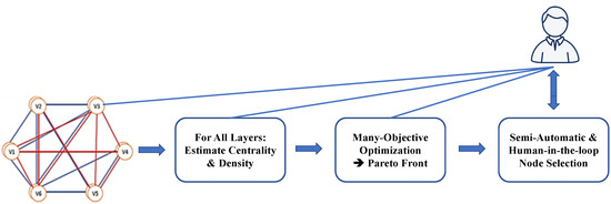
Figure 1. Overview on the procedural steps of the proposed approach: first, centralities and densities are estimated before many-objective optimization is applied in order to obtain the Pareto Front, i.e., the set of less important nodes. Finally, these are assessed in a human-in-the-loop approach.

3.2. Multi-Layer Networks

A multi-layer network (with a multiplex network as a special case) consists of multiple layers, modeling multiple relations. More formally, it can be defined as a graph $G=(V,E_l),l=1\dots m$ composed of $n=\left|V\right|$ nodes and m different link sets for those nodes, which we call layers; accordingly, the set of nodes is denoted by V and the sets of links are modeled by $E_l$, $l\in \{1\dots m\}$. Furthermore, distinguishing between the different layers and modeling them as separate graphs, a multiplex network then can be represented formally as $G=(G_1,G_2,\dots ,G_l,\dots ,G_m)$, where $G_i=(V_i,E_i)$, with $V_i\subseteq V$ and $E_i$ models the edges of the ith layer. For a multiplex network, it holds that $V_i=V_j$ for $i\ne j$. A visual depiction of the network with different layers is shown in Figure 2.

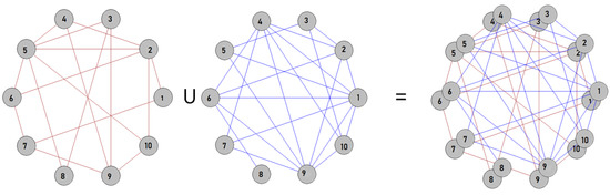
Figure 2. Depiction sketch of a multi-layer network consisting of ten nodes, with two types of different links. The different sets of links in this network are illustrated by different colors (of the respective links/edges).

Each network $G_l$ is represented by an adjacency matrix $A_l$ with entries $a_{ij}^l=W_{ij}^l>0$ if there is a positive weight of the link between nodes $v_{il},v_{jl}\in E_l$ in layer l and $a_{ij}^l=0$ otherwise. We use this representation to simplify the formalization of weighted multiplex networks by only considering edges with an integer weight larger or equal to zero between any pair of nodes $v_{il}$ and $v_{jl}$ in a layer l.

3.3. Network Centrality

To find the most influential node in a network, we can utilize the notion of network centrality. This is formalized using different network centrality metrics. In everyday life, for example, we perceive a person or some people to be very important in a community or in an organization if in some way those have a certain influence on others or can generate important decision for a community. Identifying important person or organizations can then be considered as identifying key players in a community.

Network centrality methods enable the identification of such key players or most influential nodes in a social setting [56,57]. They include, e.g., the following centrality measures:

• closeness centrality, measuring the distance from a specific node to all other nodes [58];
• betweenness centrality, taking into account the number of shortest paths past the certain nodes in the network [59];
• eigenvector centrality, considering the number of links from other nodes, their importance, and to how many these nodes themselves point to, c.f., [60]; and
• degree centrality, centering on the number of connected peers for a node [61,62].

For our proposed approach, we consider eigenvector centrality which is computed for each layer of the network. We applied eigenvector centrality, since this precisely corresponds to our intuition for estimating the notion of connections to important nodes and/or parts of the network, which is relevant for anomaly detection. However, our method can potentially also be adapted to other centrality measures, e.g., see those above.

The eigenvector centrality can be defined as follows: For a given graph G: = $(V,E)$ with $\left|V\right|$ denoting the number of nodes, let $A=\left(a_{v,t}\right),$ $v\in \{1,\dots ,|V\left|\right\}$, $t\in \{1,\dots ,|V\left|\right\}$ be the adjacency matrix, i.e., $a_{v,t}=1$ if vertex v is linked to vertex t, and $a_{v,t}=0$ otherwise.

The relative centrality score of vertex v is defined as

$$x_v=\frac{1}{\lambda }\sum _{t\in M\left(v\right)}{x}_t=\frac{1}{\lambda }\sum _{t=1}^{\left|V\right|}{a}_{t,v}{x}_t,$$

where $M\left(v\right)$ is a set of the neighbors of v and $\lambda$ is a constant.

Furthermore, the eigenvector centrality in vector notation can be written as follows: $Ax=\lambda x.$ It is clearly defined that x is an eigenvector of A. Since there could be many eigenvectors of A, by convention, the eigenvector that corresponds to the largest eigenvalue is considered. There are two important factors that influence the eigenvector centrality of each node: (1) the number of neighbors that point to the node and (2) the weight of neighbors that point to the node.

Furthermore, there is also a possibility that nodes with a larger number of neighbors have a lower eigenvector centrality compared to nodes with fewer neighbors. This situation can occur, for example, when the neighbors of the less connected node have higher weights.

3.4. Centrality-Based Many-Objective Optimization Approach

For many-objective optimization of the network centrality, we define one objective function for each layer; per layer, our method is applied to minimize the eigenvector centrality of that layer, while overall, all layers are obviously taken into account by our proposed many-objective optimization approach. Using this method, for a multiplex network G with layers $G_1,\dots ,G_m$, m is thus defined as the number of objective functions.

Obviously, each node in each layer of the network can have a different centrality—either high or low and dominated or non-dominated. The node centrality is said to be non-dominated if there is no other point better than or equal to the centralities in different layers and better in at least one criterion or in one layer. For computing the non-dominated subset from a finite set of n solutions, the algorithm by Kung, Luccio, and Preparata is the fastest known approach [63]. It accomplishes this task with a time complexity in $O(nlogn)$ for $m=2,3$ and $O\left(n{(logn)}^{m-2}\right)$ for $m>3$. For our proposed approach, we compute the Pareto Front using many-objective optimization (by minimizing eigenvector centrality) to find the set of non-dominated solutions, i.e., the set of nodes with very low importance in the multi-layer network. The set of nodes in the resulting Pareto Front, i.e., the set of non-dominated solutions, is then the basis to select suspected anomalous nodes.

3.5. Statistical Analysis Based on Edge-Density

For statistical analysis of the nodes, we apply the nodes’ mean centrality and standard deviation for a respective layer to derive a specific score, as discussed below. We summarize basic notions according to the standard formalizations in the following.

In terms of arithmetics, the mean or average is usually denoted by $\overline{x}$ or $\mu$, considering the sum of the sample values divided by the number of items in the sample, i.e.,

$$\mu =\frac{1}{n}\left(\sum _{i=1}^n{x}_i\right)=\frac{x_1+x_2+\cdots +x_n}{n},$$

as the sum of the sampled values $x_i$ divided by the number of items n in the sample.

The standard deviation

$$\sigma =\sqrt{\frac{1}{n-1}\sum _{i=1}^n{(x_i-\mu )}^2},$$

measures the spread of the sample compared to the mean. Thus, it can be interpreted as how the measurements for a group are spread out from the average (mean) or expected value. A low standard deviation means that most of the numbers are close to the average. A high standard deviation means that the numbers are more spread out. Furthermore, we include another parameter, i.e., the edge density, which measures the fraction of present to possible edges. In a dense graph, the number of edges is close to the maximal number of edges. In contrast, a graph with only a few edges is then a sparse graph. For undirected simple graphs, the (graph) density is defined as $D=\frac{2\left|E\right|}{\left|V\right|\left(\right|V|-1)}.$ For a directed graph, this graph density is divided by two in order to take the directionality of edges into account.

3.6. Assessing Anomalous Nodes

For the final step in identifying a set of nodes that have no connection or have very low centrality in a high density layer, it is necessary to consider the density of the layer and to take the less important nodes, which are far from the mean in that layer, into account. In the following, we describe a special score to be applied, which we propose for indicating a node as an anomaly, the so-called ACE score (Anomaly candidate based on Centrality Evaluation).

The ACE score considers the mean and standard deviation of the centrality of all nodes in a specific layer (of the multiplex network), e.g., one which has very high edge density compared to other layers. Using the ACE score for the set of nodes on the Pareto Front, we chose those with the highest ACE score or those that are very close to this score and are far from the mean $\mu$ in each layer. Then, these nodes were indicated as anomalous candidate nodes. These candidates can then be further assessed and inspected in the described human-centered approach. More formally, the ACE score for node v in layer l is defined as follows:

$$ACE(v,l)=\left(\frac{{\mu }_l-x_{vl}}{{\sigma }_l}\right)D_l,$$

where ${\mu }_l$ is the mean nodal centrality in layer l, $x_{vl}$ is the centrality of each node/vertex v in layer l, ${\sigma }_l$ is the standard deviation, and $D_l$ denotes the edge density of layer l.

4. Results

For our evaluation, we discuss the experimentation performed in four experiments and case studies using a synthetic as well as several real-world networks. Those include (face-to-face) social interactions, a trade interaction network, as well as social media induced networks. It is important to note that, in this paper, we focus on the task of group anomaly detection, specifically with a semiautomatic human-in-the-loop approach. To the best of the authors’ knowledge, this is a novel methodological focus, lacking standard methods for comparison. Therefore, in our experimentation and discussion, we focus on the evaluation of our proposed method, analyzing and discussing our results in detail, including qualitative results and insights in the context of several case studies on real-world datasets. We first provide an overview on the different network datasets before we provide our analysis results, discussing them in detail in context.

4.1. Datasets—Networks

For the synthetically generated network, we applied the Erdős and Rényi models since these are standard network generation models that are also simple to interpret. For the real-world networks, we utilized a range of datasets with different sizes and characteristics, also covering different domains. We applied the following datasets, as summarized in Table 1, which are also publicly available:

Table 1. Summary: statistical overview on the applied networks, describing the overall number of nodes, the number of layers, and the overall number of edges of the respective multiplex networks.

Network Type	Number of Nodes	Number of Layers	Number of Edges
Synthetic	100	5	8158
CS-Aarhus	61	5	620
Kapferer-Tailor	39	4	552
Social Media	6407	3	74,862
Trade Network	207	11	148,727

• a standard multiplex network dataset from Aarhus university [64,65],
• the Kapferer Tailor Shop multiplex network [66,67],
• a multi-layer network modeling world trade [8,29,68], and
• a multi-layer social network induced by social media (FriendFeed, Twitter, Youtube) [1,3,69].

4.2. Case Study I: Synthetic Multi-Layer Networks

In our first case study for evaluating our approach, we focus on synthetically generated networks. These are generated via a random graph according to the Erdős and Rényi model. In this complete graph model, each edge has a probability of $1-p$ to be removed from the network. By varying the probability and number of nodes, we can generate different networks and layers, respectively.

We generated networks with a specific number of nodes ($n=100$) and link probabilities ranging from $p=0.03$ to $p=0.3$; for the number of layers, we chose $l=5$ layers. We denote the layers with $g_1$ to $g_5$. Table 2 provides an overview on the respective network statistics. Figure 3 shows the applied synthetic network based on Erdős-Rényi graph generation. Each layer corresponds to one synthetic network with different link probabilities $p\in \{0.03,0.05,0.20,0.25,0.30\}$. We performed a round of experiments, and take this specific instantiation as an example to demonstrate the methodological approach. Other instantiations, e.g., varying the number of layers, showed similar results.

Table 2. Statistical characterization: synthetic multiplex network generated via an Erdős-Rényi graph generation process. Each layer of the network corresponds to one synthetic network with the link probability $p\in \{0.03,0.05,0.20,0.25,0.30\}$.

Layer	$\mathit{\mu }$	$\mathit{\sigma }$	D
L1 ($\mathit{p}=\mathbf{0.03}$)	0.194114	0.1911789	0.028889
L2 ($\mathit{p}=\mathbf{0.05}$)	0.34386	0.1979547	0.056566
L3 ($\mathit{p}=\mathbf{0.20}$)	0.674128	0.1472402	0.198384
L4 ($\mathit{p}=\mathbf{0.25}$)	0.651931	0.1232115	0.235556
L5 ($\mathit{p}=\mathbf{0.30}$)	0.726498	0.1220831	0.29899

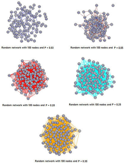
Figure 3. Synthetic network generated by an Erdős Rényi random graph generation strategy. Each layer consists of 100 nodes. For the different layers (1–5), layer 1 top left, layer 2 top right, etc. to bottom layer 5, we applied different link probabilities p for generation, thus each layer has a different edge-density.

For our example case, as a result of the estimation of eigenvector centrality and the application of many-objective optimization for synthetics networks, we detected 38 nodes in the Pareto Front, c.f., Table 3. Applying our selection methodology described in Section 3, we started with those nodes in the Pareto Front in order to identify candidate nodes as sets of anomalous nodes. Therefore, starting with these 38 nodes, we observe a set of nodes with very high ACE score values or some nodes that are very close to these and show a large deviation from the respective centrality mean $\mu$. In particular, we took those nodes with very high ACE score in specific consideration, where we observe them being contained in the layers that have high density D. In our case, these are the layers $g_3$, $g_4$, and $g_5$. As a result, we can identify six nodes (35, 39, 48, 68, and node 99), which were then categorized as anomalous nodes.

Table 3. Synthetic network with 100 nodes consisting of five layers, with 38 nodes in the Pareto Front.

	L1	L2	L3	L4	L5	Node ID	Level
1	0.238847	0.278869	0.586341	0.642287	0.924788	1	1
2	0.191164	0.174877	0.687559	0.675231	0.75411	2	1
3	1.25E-17	0.416006	0.75482	0.474529	0.757621	3	1
4	1.25E-17	0.401982	0.551425	0.662649	0.79923	4	1
5	1.25E-17	0.213736	0.7307	0.617663	0.897725	9	1
6	1.25E-17	0.125957	0.790128	0.567224	0.633085	11	1
7	0.262506	0.191137	0.51756	0.589189	0.7169	13	1
8	0	0.476025	0.784085	0.658702	0.609807	15	1
9	0	0.613012	0.550916	0.764643	0.708011	20	1
10	1.25E-17	0.336907	0.520273	0.761882	0.922795	24	1
11	0	0.148321	0.698593	0.703381	0.876309	26	1
12	0.957554	0.045396	0.676144	0.46505	0.723078	27	1
13	1.25E-17	0.130615	0.490935	0.73268	0.893768	28	1
14	1.25E-17	0.085199	0.617385	0.567831	0.848255	31	1
15	1.25E-17	0.241517	0.453056	0.851897	0.617858	32	1
16	0	0.727116	0.410735	0.713941	0.911162	33	1
17	0	0.634736	0.848863	0.712245	0.491106	35	1
18	1.25E-17	0.382777	0.500778	0.688717	0.72154	38	1
19	0.48938	0.398631	0.45282	0.44327	0.752472	39	1
20	1.25E-17	0.133565	0.626805	0.62483	0.912015	44	1
21	0.48938	0.915795	0.637746	1	0.730629	46	1
22	0.199638	0.115416	0.588351	0.522453	0.499154	48	1
23	0.199638	1	0.616606	0.736292	0.885649	51	1
24	0	0.502089	0.69011	0.70434	0.66845	56	1
25	0.468608	0.201663	0.858988	0.452652	0.66817	60	1
26	0.515027	0.205772	0.948334	0.664673	0.786612	61	1
27	1.25E-17	0.174322	0.840323	0.598745	0.637779	63	1
28	1.25E-17	0.439402	0.381991	0.710902	0.693444	68	1
29	1.25E-17	0.671161	0.779929	0.687363	0.80535	69	1
30	0.128465	0	0.69584	0.702146	0.915057	70	1
31	0	0.164657	0.578598	0.813264	0.685314	73	1
32	1.25E-17	0.1548	0.582233	0.578118	0.894428	79	1
33	0.052406	0.35037	0.547268	0.739041	0.81452	83	1
34	0	0.912872	0.592001	0.73704	0.904102	88	1
35	0	0.21671	0.774421	0.797105	1	89	1
36	1.25E-17	0.067691	0.575705	0.601373	0.643516	92	1
37	1	0.178088	0.40133	0.739926	0.676465	99	1
38	0	0.558778	0.494943	0.764686	0.827497	100	1

As can be observed in Table 3 and Table 4 and Figure 3, in this way, we selected the nodes with the highest ACE score that are also in the Pareto Front, focusing on the denser layers, while the low-density layers are neglected since these also feature quite low ACE scores. Intuitively, this makes sense since a node with a low connectivity and/or high eigenvector centrality on a layer with higher density then gets a higher chance to be proposed as an anomalous node. It is important to note that layers $g_1$ and $g_2$ feature some unconnected nodes, which can then be indicated as anomaly candidates for these layers based on a connectivity criterion as well. Such a (simple) criterion can of course be implemented complementing the Pareto-front-based selection. However, in our many-objective optimization approach, we consider all layers at the same time to first find initial candidates on the Pareto Front by minimizing eigenvector centrality, which are then refined using further criteria such as density and connectivity, which are formalized in the novel ACE score.

Table 4. ACE score of the synthetic/artificial network with 100 nodes consisting of five layers.

No	L1		L2		L3		L4		L5
	ACE score	Node	ACE score	Node	ACE score	Node	ACE score	Node	ACE score	Node
1	0.003489	7	0.029332	22	0.39361	68	0.520676	40	0.576491	35
2	0.003489	12	0.029332	70	0.37581	66	0.398917	39	0.556781	48
3	0.003489	15	0.028154	57	0.367554	99	0.38098	60	0.512226	49
4	0.003489	19	0.026904	41	0.36481	77	0.373612	85	0.49261	71
5	0.003489	20	0.025192	49	0.363811	71	0.357277	27	0.364353	75
6	0.003489	21	0.024367	96	0.362636	78	0.339156	3	0.332967	14
7	0.003489	22	0.024012	21	0.354883	33	0.290516	93	0.327641	64
8	0.003489	26	0.023848	50	0.300521	8	0.278613	78	0.323315	43
9	0.003489	33	0.023426	87	0.298178	39	0.270124	47	0.303674	30
10	0.003489	35	0.023066	78	0.297861	32	0.26853	18	0.301767	98
11	0.003489	36	0.022582	14	0.249337	50	0.265734	30	0.287986	66

Overall, it is important to note that all of the steps of this process occur transparently, i.e., the initial candidates can be inspected and validated by the human-in-the-loop and guided by visualizations such as those given in Figure 3. This is an important and relevant feature of our approach regarding interpretability and explainability, as also discussed in the process model in Section 3.

4.3. Case Study II: Aarhus Real-World Multi-Layer Network

In our second experiment, we consider the analysis of a first real-world multiplex network. The network application context relates to the scope of social interactions, i.e., interactions in a departmental context between people working at that department [64,65]. Here, we observed slightly different patterns compared to the synthetic network data, which we discuss in detail below.

The applied network data consist of five layers modeling online and offline relationships (Facebook, Leisure, Work, Co-authorship, and Lunch) between the employees of the Computer Science department at Aarhus University. The network includes 61 nodes, representing the respective members at the department. Figure 4 depicts the individual layers of the multiplex network, representing the individual relationships. We observe a rather relative dense structure in layer 5 compared to the other layers, this is also summarized in Table 5 where we present a statistical overview on the network and its layers, respectively.

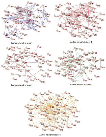
Figure 4. Aarhus multiplex network. Here, we show the individual layers of the network, where the different sets of edges of each layer are also illustrated via different colors for the connected edges.

Table 5. Statistical characterization: Aarhus multiplex network.

Layer	$\mathit{\mu }$	$\mathit{\sigma }$	D
Layer 1	0.257986	0.291311	0.1054645
Layer 2	0.273081	0.331148	0.06775956
Layer 3	0.073182	0.240734	0.01147541
Layer 4	0.176249	0.22261	0.04808743
Layer 5	0.266831	0.20674	0.1060109

Figure 5 shows a detailed view on layer 5, i.e., the densest layer. Here, we can already observe some interesting findings regarding the connection structure, i.e., regarding relatively loosely connected nodes and one unconnected node. This will be useful when interpreting our results, which we will discuss in the following.

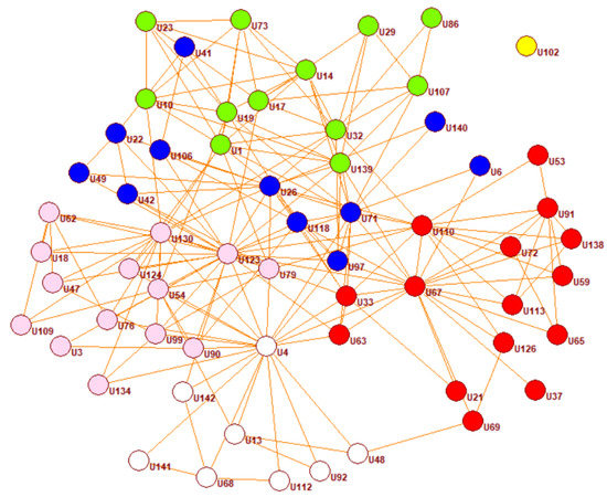
Figure 5. Visualization of the Aarhus network, i.e., layer 5. Here, we observe clearly how the nodes connect to others with many connections, few connections, or even without a single connection.

As result of estimating the centrality for all nodes in all layers and applying many-objective optimization through minimization, we found a Pareto Front that consists of six nodes. As shown in Figure 6, these are the nodes 1, 8, 12, 14, 37, and 60. For determining the nodes to be categorized as anomalous nodes, we considered the high density D layers as a basis to find nodes with the highest ACE score. Additionally, we considered the ones closest to the highest ACE score and far from the mean $\mu$, being contained in the Pareto Front. In Figure 6, we show a visualization of the different layers and the Pareto Front.

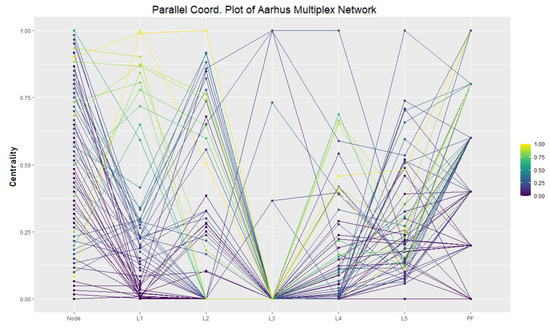
Figure 6. Pareto Front chart for the Aarhus multiplex network and the different layers ($L1-L5$): it depicts the Pareto Front (PF) based on minimization of the nodes’ centrality on the right side of the picture; the PF for the minimization is shown in the lower part of the vertical PF line.

From those nodes in the Pareto Front shown in Table 6, we assessed those with the highest ACE score in each layer—these are summarized in Table 7. As we can see in the table, in layer 1, the highest score is achieved by node 60, while in layer 2, there are nodes 1 and 14; in layer 3, there are nodes 4, 8, 12, and 14; in layer 4, there are nodes 1, 14, and 60; and finally, in layer 5, there is node 1. Since layer 3 exhibits a very low density D, we did not consider this layer as a high indicator in consideration in order to find anomalous nodes. Additionally, as can be seen from the scores and the different layers, we can actually focus on those nodes that occur in more than two layers as interesting candidates, which also supports our intuitions. Therefore, in this way, we can actually collect “evidence” in this network towards designating nodes as anomalous from several layers of the network.

Table 6. Pareto Front—many-objective centrality optimization on the Aarhus multiplex network.

Aarhus Pareto Front
No	L1	L2	L3	L4	L5	Node	Label	Level
1	0.0205957	0	8.12E-17	0	1.56E-17	1	U102	1
2	0.0092203	0.3276641	0	0.1228	0.4873511	8	U1	1
3	0.0087273	0.2510376	0	0.1232	0.1325338	12	U29	1
4	0.0199306	0	0	0	0.0877403	14	U41	1
5	0.0027204	0.385105	0	0.1907	0.2563836	37	U10	1
6	3.06E-17	0	8.12E-17	0	0.1415063	60	U140	1
7	0.0493792	0.2837498	0	0	0.2205827	4	U106	2
8	0.021995	0	0	0	0.4590027	6	U118	2
…	…	…	…	…	…	…	…	…
…	…	…	…	…	…	…	…	…
…	…	…	…	…	…	…	…	…
47	0.0092	0	8.12E-17	0.29	0.23918	20	U17	4
48	0.13002	0	0.36603	0.396	0.14978	48	U138	4
49	0.27625	0.73729	8.12E-17	0	1	7	U123	5
50	0.29799	0.82106	8.12E-17	0.333	0.2724	19	U124	5
51	0.23158	0.30094	8.12E-17	0.417	0.13512	17	U59	5
52	1	0.50403	8.12E-17	0.4	0.11494	24	U109	5
53	0.71836	0.59922	8.12E-17	0.218	0.12304	29	U3	5
54	0.90271	0	8.12E-17	0.653	0.25754	35	U90	5
55	0.86681	0.74213	0	0.414	0.24717	33	U76	5
56	0.41465	0.9133	8.12E-17	0.017	0.70072	44	U4	5
57	0.33325	0.7789	8.12E-17	0.1	0.65743	51	U67	5
58	0.98973	1	8.12E-17	0.456	0.48118	34	U79	6
59	0.23158	0.85764	1	1	0.18967	23	U91	6
60	0.87278	0.76229	8.12E-17	0.665	0.34929	31	U54	6
61	0.23263	0.65021	1	0.589	0.53389	46	U110	6

Table 7. ACE scores for the Aarhus multiplex network.

No	Aarhus L1		Aarhus L2		Aarhus L3		Aarhus L4		Aarhus L5
	ACE score	Node	ACE score	Node	ACE score	Node	ACE score	Node	ACE score	Node
1	0.0933996	60	0.05587783	1	0.0034885	4	0.03807	1	0.13682	1
2	0.0925381	2	0.05587783	2	0.0034885	6	0.03807	2	0.10696	22
3	0.0924148	37	0.05587783	3	0.0034885	8	0.03807	3	0.10384	43
4	0.0918969	41	0.05587783	6	0.0034885	10	0.03807	4	0.10052	49
5	0.0916538	42	0.05587783	10	0.0034885	11	0.03807	6	0.09659	53
6	0.0909673	5	0.05587783	11	0.0034885	12	0.03807	7	0.09659	61
7	0.0902401	12	0.05587783	14	0.0034885	13	0.03807	14	0.09568	59
8	0.0901458	45	0.05587783	18	0.0034885	14	0.03807	18	0.09313	56
9	0.090068	20	0.05587783	20	0.0034885	26	0.03807	21	0.09183	14
10	0.0900616	8	0.05587783	22	0.0034885	27	0.03807	22	0.09141	54
11	0.0897165	40	0.05587783	25	0.0034885	28	0.03807	26	0.08707	50
12	0.0861841	14	0.05587783	32	0.0034885	30	0.03807	27	0.08495	55
13	0.0861841	16	0.05587783	35	0.0034885	33	0.03807	53	0.07799	9
14	0.0859433	1	0.05587783	36	0.0034885	36	0.03807	54	0.07789	24
15	0.0854367	6	0.05587783	38	0.0034885	37	0.03807	57	0.07567	38
16	0.0854367	10	0.05587783	40	0.0034885	38	0.03807	59	0.07373	29
17	0.0854367	11	0.05587783	41	0.0034885	39	0.03807	60	0.07278	25
18	0.0810578	22	0.05587783	42	0.0034885	54	0.03774	61	0.06886	12
19	0.0788396	13	0.05587783	43	0.0034885	55	0.03607	55	0.06754	17
20	0.0755227	4	0.05587783	45	0.0034885	1	0.03488	10	0.06678	58

As a consequence, we can identify four nodes out of six nodes in the Pareto Front to be selected as candidate anomalous nodes in our semiautomatic human-centered process, as we have discussed above. As an outcome, the designated final set of anomalous nodes is given by nodes 1, 12, 14, and 60. In the social context, this then indicates, for example, that node 1, node 12, node 14, and node 60 are not very active in the interaction with their colleague in terms of special interactions (layer1 = Facebook, layer 2 = Leisure, layer 3 = Work, layer 4 = Co-authorship, and layer 5 = Lunch): node 60 and node 12 are very rare in interactions with their colleagues on Facebook, and node 1 and node 14 are not very active in communication with their colleague related to leisure and co-authorship. Additionally, node 1 shows little interaction in leisure and co-authorship and is less active in interacting with his colleagues regarding lunch. The analysis process described above provides for a human-centered interpretable and explainable approach since simple network metrics and topological indicators can be easily inspected in context on the multiplex network, making use of the visualization of different layers and contextual inspection of their parameters [55,70].

4.4. Case Study III: Real-World Multi-Layer Network—Kapferer Tailor Shop

The third experiment concerns another well-known social network dataset in a multi-relational context [66,67]. This well-known social network dataset was collected by Bruce Kapferer himself in Zambia (June to August 1965), c.f., [66]. The dataset involves interactions among workers in a tailor shop. An interaction is defined by Kapferer as “continuous uninterrupted social activity involving the participation of at least two persons” (p. 163, [66]); only transactions that were relatively frequent are recorded. All of the interactions in this particular dataset are “sociational”, as opposed to “instrumental”. Kapferer explained the difference (p. 164, [66]) as follows: “I have classed as transactions which were sociational in content those where the activity was markedly convivial such as general conversation, the sharing of gossip and the enjoyment of a drink together. Examples of instrumental transactions are the lending or giving of money, assistance at times of personal crisis and help at work.” [66].

Kapferer also observed and recorded instrumental transactions, many of which are unilateral (directed) rather than reciprocal (undirected), though those transactions are not recorded here. In addition, there was a second period of data collection, from September 1965 to January 1966, but these data are also not recorded here. All data are given in Kapferer’s 1972 book [66] on pp. 176–179. Kapferer observed different types of interactions in two different time intervals, which were seven months apart. Each layer of the network denotes a different type of interaction at the shop, i.e., sociational (friendship and socioemotional) and instrumental (work- and assistance-related).

Our applied dataset was taken from the well-known Kapferer multi-layer network data. The network data includes 39 individuals who are represented as nodes in the network. Table 8 provides a statistical characterization of the network and its layers. Figure 7 shows a visualization of the different layers and the Pareto Front using a Parallel Coordinates plot. Here, we can clearly identify the anomaly candidates (on the right) obtained by our approach.

Table 8. Statistical characterization: Kapferer Tailor Shop multiplex network.

Layer	$\mathit{\mu }$	$\mathit{\sigma }$	D
Layer 1	0.3854688	0.2125424	0.4264507
Layer 2	0.4899419	0.2459141	0.6018893
Layer 3	0.260266	0.2709372	0.1470985
Layer 4	0.2506608	0.2362966	0.1983806

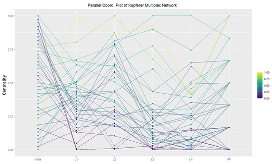
Figure 7. Pareto Front chart for the Kapferer multiplex network and the different layers ($L1-L4$): it depicts the Pareto Front (PF) based on minimization of the nodes’ centrality on the right side of the picture; the PF for the minimization is shown in the lower part of the vertical PF line.

From our experimentation utilizing many-objective optimization, we detected eight nodes in the Pareto Front. These are Donald, Mateo, Chipalo, Paulos, Sign, Zakeyo, Adrian and Kallundwe; see Table 9 for details. By calculating and identifying the highest ACE score in each layer except in the layer with the lowest of the density, we finally obtained the following nodes: Sign, Donald, Zakeyo, and Chipalo have the highest ACE-Score in layers 1, 2, and 4 respectively; here, we neglect layer 3 as it is the one with the lowest network density. Therefore, Sign, Donald, Zakeyo, and Chipalo are finally selected as anomalous nodes in the network. For a detailed view on the statistics, we refer to Table 10.

Table 9. Pareto Front and network centralities of the Kapferer Tailor Shop multiplex network.

No	L1	L2	L3	L4	Node	Label	Level
1	0.397101	0.076899	0.227271	4.36E-19	6	DONALD	1
2	0.17709	0.255465	1.57E-17	0.075394	8	MATEO	1
3	0.059998	0.341019	1.57E-17	0.255959	10	CHIPALO	1
4	0.297021	0.373386	1.57E-17	0.034534	18	PAULOS	1
5	0.013455	0.084826	0.028562	0.160698	20	SIGN	1
6	0.022149	0.259987	0.006686	0.078514	22	ZAKEYO	1
7	0.154452	0.480842	1.57E-17	2.47E-18	26	ADRIAN	1
8	0.143018	0.172989	0.020164	2.47E-18	27	KALUNDWE	1
9	0.481191	0.104547	0.228507	0.050905	4	SEAMS	2
10	0.141911	0.352355	0.122665	0.147189	17	ENOCH	2
11	0.237573	0.803971	0.105287	0.141186	25	MESHAK	2
12	0.235435	0.23692	0.158304	0.012102	23	BEN	2
13	0.372248	0.28798	0.045572	0.081653	35	CHRISTIAN	2
14	0.446693	0.310456	0.060973	0.077575	38	CHILUFYA	2
15	0.250912	0.241652	0.07816	1.14E-17	39	MABANGE	2
16	0.201821	0.607807	0.23093	0.353406	1	KAMWEFU	3
17	0.241237	0.655692	0.203435	0.623016	5	CHIPATA	3
18	0.276116	0.307887	0.302346	0.038746	15	NYIRENDA	3
19	0.307472	0.335643	0.180225	0.252708	28	MPUNDU	3
20	0.351199	0.284229	0.344007	0.224243	37	ANGEL	3
21	0.417402	0.403791	0.084483	3.21E-17	33	CHOBE	3
22	0.40163	0.475965	0.604055	0.304077	9	CHILWA	4
23	0.318112	0.617183	0.282275	0.255397	2	NKUMBULA	4
24	0.373917	0.571605	0.240467	0.491226	14	LWANGA	4
25	0.430833	0.481783	0.172491	0.237627	29	JOHN	4
26	0.438643	0.721808	0.09152	0.188956	21	KALAMBA	4
27	0.495024	0.405638	0.093042	0.025297	31	WILLIAM	4
28	0.467563	0.418168	0.129541	0.092453	36	KALONGA	4
29	0.637761	0.658291	0.77509	0.411734	12	ZULU	5
30	0.333699	0.666146	0.432999	0.649743	7	NKOLOYA	5
31	0.508462	0.881521	0.277381	0.506618	24	IBRAHIM	5
32	0.510248	0.730396	0.252753	0.268102	30	JOSEPH	5
33	0.64177	0.543767	0.299718	0.303266	32	HENRY	5
34	0.666847	0.649858	0.134423	0.455691	34	MUBANGA	5
35	0.677078	0.792611	1	1	11	LYASHI	6
36	0.514091	0.810266	0.433572	0.390044	13	HASTINGS	6
37	1	0.877987	0.92856	0.431482	16	CHISOKONE	7
38	0.585384	0.826399	0.900669	0.744139	3	ABRAHAM	7
39	0.806727	1	0.674242	0.412089	19	MUKUBWA	7

Table 10. Anomalous nodes of the Kapferer Tailor Shop multiplex network that are extracted from the Pareto Front based on the ACE score.

No	Kapferer L1		Kapferer L2		Kapferer L3		Kapferer L4
	ACE L1	Node ID	ACE L2	Node ID	ACE L3	Node ID	ACE L4	Node ID
1	0.746419	SIGN	1.010946	DONALD	0.141305	MATEO	0.21044	DONALD
2	0.728975	ZAKEYO	0.991545	SIGN	0.141305	CHIPALO	0.21044	ADRIAN
3	0.653032	CHIPALO	0.943277	SEAMS	0.141305	PAULOS	0.21044	KALUNDWE
4	0.488681	ENOCH	0.775762	KALUNDWE	0.141305	ADRIAN	0.21044	MABANGE
5	0.48646	KALUNDWE	0.619287	BEN	0.137675	ZAKEYO	0.21044	CHOBE
6	0.463518	ADRIAN	0.607705	MABANGE	0.130357	KALUNDWE	0.20028	BEN
7	0.418096	MATEO	0.573896	MATEO	0.125798	SIGN	0.189202	WILLIAM
8	0.368476	KAMWEFU	0.562828	ZAKEYO	0.116563	CHRISTIAN	0.181447	PAULOS
9	0.301032	BEN	0.503495	ANGEL	0.108201	CHILUFYA	0.177911	NYIRENDA
10	0.296742	MESHAK	0.494314	CHRISTIAN	0.09887	MABANGE	0.167703	SEAMS
11	0.289391	CHIPATA	0.445591	NYIRENDA	0.095437	CHOBE	0.147144	MATEO
12	0.269979	MABANGE	0.439303	CHILUFYA	0.091617	KALAMBA	0.145312	CHILUFYA
13	0.219408	NYIRENDA	0.377656	MPUNDU	0.09079	WILLIAM	0.144524	ZAKEYO
14	0.177464	PAULOS	0.364497	CHIPALO	0.084142	MESHAK	0.141889	CHRISTIAN
15	0.156495	MPUNDU	0.336752	ENOCH	0.074707	ENOCH	0.132822	KALONGA
16	0.135147	NKUMBULA	0.285278	PAULOS	0.070974	KALONGA	0.091908	MESHAK
17	0.103872	NKOLOYA	0.210859	CHOBE	0.068323	MUBANGA	0.086868	ENOCH
18	0.068759	ANGEL	0.206339	WILLIAM	0.055357	BEN	0.075528	SIGN
19	0.026526	CHRISTIAN	0.175672	KALONGA	0.047655	JOHN	0.051804	KALAMBA
20	0.023177	LWANGA	0.03421	CHILWA	0.043456	MPUNDU	0.022179	ANGEL
21	$-0.02334$	DONALD	0.022272	ADRIAN	0.030855	CHIPATA	0.010942	JOHN
22	$-0.03243$	CHILWA	0.01997	JOHN	0.017914	DONALD	$-0.00172$	MPUNDU
23	$-0.06407$	CHOBE	-0.13174	HENRY	0.017243	SEAMS	$-0.00398$	NKUMBULA
24	$-0.09102$	JOHN	-0.19988	LWANGA	0.015927	KAMWEFU	$-0.00445$	CHIPALO
25	$-0.10669$	KALAMBA	-0.28848	KAMWEFU	0.010749	LWANGA	$-0.01464$	JOSEPH
26	$-0.12284$	CHILUFYA	-0.31143	NKUMBULA	0.004079	JOSEPH	$-0.04416$	HENRY
27	$-0.16472$	KALONGA	-0.3914	MUBANGA	$-0.00929$	IBRAHIM	$-0.04485$	CHILWA
28	$-0.19206$	SEAMS	-0.40568	CHIPATA	$-0.01195$	NKUMBULA	$-0.08626$	KAMWEFU
29	$-0.21981$	WILLIAM	$-0.41204$	ZULU	$-0.02142$	HENRY	$-0.11702$	HASTINGS
30	$-0.24678$	IBRAHIM	$-0.43127$	NKOLOYA	$-0.02285$	NYIRENDA	$-0.13523$	ZULU
31	$-0.25036$	JOSEPH	$-0.56751$	KALAMBA	$-0.04547$	ANGEL	$-0.13553$	MUKUBWA
32	$-0.25807$	HASTINGS	$-0.58853$	JOSEPH	$-0.09378$	NKOLOYA	$-0.15181$	CHISOKONE
33	$-0.40111$	ABRAHAM	$-0.7408$	LYASHI	$-0.09409$	HASTINGS	$-0.17213$	MUBANGA
34	$-0.50621$	ZULU	$-0.76861$	MESHAK	$-0.18665$	CHILWA	$-0.20196$	LWANGA
35	$-0.51425$	HENRY	$-0.78401$	HASTINGS	$-0.22476$	MUKUBWA	$-0.21489$	IBRAHIM
36	$-0.56457$	MUBANGA	$-0.8235$	ABRAHAM	$-0.27951$	ZULU	$-0.31261$	CHIPATA
37	$-0.58509$	LYASHI	$-0.94976$	CHISOKONE	$-0.34769$	ABRAHAM	$-0.33505$	NKOLOYA
38	$-0.84522$	MUKUBWA	$-0.95841$	IBRAHIM	$-0.36283$	CHISOKONE	$-0.41429$	ABRAHAM
39	$-1.23301$	CHISOKONE	$-1.2484$	MUKUBWA	$-0.40162$	LYASHI	$-0.6291$	LYASHI

4.5. Case Study IV: Real-World Multi-Layer Network of World Trade Network

In our fourth experiment, we consider a multi-layer network modeling world trade relationships. These data originate from import–export interactions on commodities between some countries of the world in 2011, c.f., [8,29,68], disaggregated for different traded commodities. This network can be defined as a multiplex network composed of many layers, where each layer is given by a different commodity. Figure 8 shows the first layer of the network. The nodes are given by the 207 countries contained. A link between two countries in a layer is given if there is trade between them in the respective commodity. The data are presented in matrix form: rows and columns represent countries, and the entries of the matrices are the volumes of trade. It is therefore a weighted multiplex network. The general classification is based on 96 different commodities. The classification was performed by grouping together similar commodities; this procedure leads to 11 aggregated ‘super-commodities’.

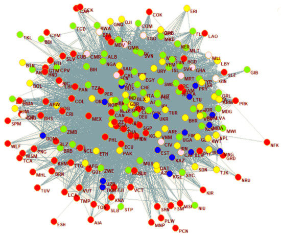
Figure 8. Visualization of world trading network on layer 1. Here, can be seen how the nodes (representing the countries) connect to the others, From the picture we can see that Ant (Antilles) node has no single connection in this layer.

In our experiment, we applied anomaly detection using the method explained above. Our results indicate a special outcome compared to other dataset—we can observe a specific special case here. Having obtained the Pareto Front and after having computed the respective ACE scores, we observe that, as a result, only one single node in the Pareto Front is provided, c.f., Table 11. Therefore, assessing a set of nodes using the ACE score cannot be performed–since we only have one candidate, which is already our final result. To this end, we conclude that, for our specific case, if we found a single node in the Pareto Front, then this node has quite different characteristics compared to all other nodes. For further (but weaker) candidates, we could resort to the nodes at the second rank of the dominated solution from the Pareto Front, using the ACE score for assessment as well.

Table 11. Pareto Front of many-objective optimization regarding multiplex network centrality of the trading network.

No	L1	L2	L3	L4	L5	L6	L7	L8	L9	L10	L11	Label	Level
1	1E-18	1E-18	4E-19	9E-19	4E-19	9E-19	3E-18	2E-18	4E-19	1E-18	2E-18	‘ANT’	1
2	3E-02	3E-02	2E-02	6E-02	5E-02	5E-02	6E-03	6E-02	6E-02	1E-01	6E-02	‘CXR’	2
3	6E-03	1E-18	4E-19	5E-03	5E-03	9E-19	7E-03	1E-02	2E-02	4E-02	2E-02	‘ESH’	2
4	2E-02	3E-02	8E-02	1E-01	1E-01	8E-02	6E-02	1E-01	1E-01	2E-01	9E-02	‘TKL’	3
5	1E-02	4E-02	3E-02	4E-02	6E-02	5E-02	2E-02	4E-02	7E-02	9E-02	7E-02	‘NFK’	3
6	6E-02	2E-02	5E-02	3E-02	3E-02	4E-02	1E-02	4E-02	5E-02	9E-02	4E-02	‘SPM’	3
7	3E-02	4E-02	3E-02	2E-02	4E-02	3E-02	4E-02	3E-02	5E-02	1E-01	5E-02	‘NIU’	3
8	5E-02	1E-02	5E-02	4E-02	4E-02	3E-02	3E-02	2E-02	5E-02	8E-02	6E-02	‘TUV’	3
9	2E-02	2E-02	8E-03	2E-02	3E-02	2E-02	9E-03	2E-02	5E-02	7E-02	4E-02	‘PCN’	3
10	1E-01	2E-02	3E-02	6E-02	5E-02	3E-02	4E-02	4E-02	6E-02	1E-01	5E-02	‘FLK’	4
11	3E-02	2E-02	5E-02	6E-02	7E-02	5E-02	2E-02	5E-02	8E-02	1E-01	9E-02	‘NRU’	4
12	4E-02	4E-02	6E-02	6E-02	5E-02	7E-02	1E-02	8E-02	8E-02	1E-01	9E-02	‘MNP’	4
13	3E-02	2E-02	1E-01	9E-02	7E-02	9E-02	1E-02	6E-02	1E-01	2E-01	1E-01	‘AIA’	4
14	3E-02	3E-02	2E-02	5E-02	6E-02	3E-02	2E-02	5E-02	8E-02	1E-01	6E-02	‘CCK’	4
15	5E-02	2E-02	6E-02	6E-02	4E-02	4E-02	3E-02	4E-02	5E-02	9E-02	6E-02	‘PLW’	4
16	3E-02	3E-02	5E-02	5E-02	6E-02	5E-02	4E-02	4E-02	5E-02	8E-02	6E-02	‘WLF’	4
17	6E-02	3E-02	2E-01	2E-01	2E-01	2E-01	6E-02	1E-01	2E-01	3E-01	2E-01	‘GIB’	5
18	5E-02	5E-02	2E-01	1E-01	1E-01	1E-01	5E-02	1E-01	2E-01	2E-01	1E-01	‘TCA’	5
19	7E-02	8E-02	2E-01	1E-01	1E-01	7E-02	2E-02	8E-02	2E-01	3E-01	1E-01	‘STP’	5
20	5E-02	5E-02	8E-02	8E-02	7E-02	6E-02	3E-02	7E-02	9E-02	2E-01	8E-02	‘MSR’	5
21	8E-02	3E-02	5E-02	8E-02	6E-02	5E-02	2E-02	6E-02	9E-02	2E-01	9E-02	‘SHN’	5
22	1E-01	8E-02	1E-01	9E-02	6E-02	8E-02	5E-02	7E-02	8E-02	1E-01	1E-01	‘KIR’	5
23	9E-02	3E-02	8E-02	9E-02	8E-02	7E-02	3E-02	1E-01	1E-01	2E-01	7E-02	‘COK’	5
24	9E-02	5E-02	8E-02	6E-02	9E-02	5E-02	5E-02	7E-02	7E-02	1E-01	7E-02	‘FSM’	5
25	8E-02	9E-02	2E-01	2E-01	2E-01	2E-01	7E-02	1E-01	2E-01	3E-01	2E-01	‘LCA’	6
26	8E-02	8E-02	3E-01	2E-01	2E-01	2E-01	5E-02	3E-01	2E-01	3E-01	2E-01	‘BMU’	6
27	5E-02	1E-01	1E-01	2E-01	2E-01	1E-01	1E-01	1E-01	2E-01	2E-01	2E-01	‘ERI’	6
28	9E-02	2E-01	9E-02	1E-01	1E-01	9E-02	4E-02	1E-01	2E-01	2E-01	2E-01	‘TMP’	6
29	6E-02	9E-02	2E-01	2E-01	2E-01	2E-01	4E-02	2E-01	2E-01	3E-01	2E-01	‘CYM’	6

4.6. Case Study V: Real-World Multi-Layer Social Media Network—FriendFeed, Twitter, Youtube (FFTWYT)

For the experiments in this final case study, we focused on a multi-layer network in the context of social media—considering networks on FriendFeed, Twitter, and Youtube (FFTWYT). The respective anonymized dataset [1,3,69] was obtained starting from FriendFeed, i.e., a social media aggregator. In the following, we summarize the data collection and aggregation according to [1,3,69]: In the FriendFeed system, the users can directly post messages and comment on other messages; in addition, they can also register their accounts on other systems. For constructing the dataset, the FriendFeed social media aggregator was used to align users also registered on the respective other platforms (http://multilayer.it.uu.se/datasets.html; last accessed, 17 November 2020).

Using the FriendFeed information about users who registered exactly one Twitter account that was associated to exactly one FriendFeed account, two layers can be inferred (ff-tw); in addition, an additional YouTube layer (ff-tw-yt) could be constructed using the respective links to YouTube, c.f., [1,3,69]. This results in three layers in total. The real network data applied features a total number of 6407 nodes and 74,862 edges. Table 12 shows a statistical characterization and network metrics of the different layers.

Table 12. Statistical characterization: social media multiplex network (ff-tw-yt). $\mu$ is the mean centrality of the layer, $\sigma$ is the standard deviation of the centrality, and D is the density of the layer.

Layer	$\mathit{\mu }$	$\mathit{\sigma }$	D
Layer 1 for Facebook	0.005483732	0.0327055	0.0007777407
Layer 2 for Twitter	0.01483255	0.05158178	0.001031278
Layer 3 for YouTube	0.001921569	0.03622121	1.499258E-05

From the Pareto Front of the social media network data, we obtained 7 nodes, i.e., nodes 143, 1101, 1102, 2551, 3418, 4391, and 4497, as shown in Table 13. While the many-objective optimization approach works fine on the dataset, it is easy to see that layer 1 (Youtube) does not contribute much regarding the findings, since the centralities are mostly zero due to the sparseness (low density) of the network. Therefore, we consider the ACE score only with the layer of high edge density edge, i.e., focusing on the FriendFeed and Twitter layers (layer 2 and layer 3). Due to the very large number of nodes, we show a summary of the detailed results in Table 14. As the result, from layer 2, we can observe that nodes in the Pareto Front with high ACE scores are nodes 143, 1101, and 1102. In addition, when we compute the ACE score in layer 3, we can see that the nodes in the Pareto Front with high ACE score are the nodes 1101, 1102, and 2551. Therefore, taking both these layers into account, we determined the final set of anomalous candidate nodes from this social media multiplex network as the nodes 143, 1101, 1102, and 2551, in total.

Table 13. Pareto Front of many-objective optimization regarding multiplex network centrality for the social media multiplex network.

NO	L1:Youtube	L2:FriendFeed	L3:Twitter	Node	Level
1	0	3.15E-19	1.77E-06	143	1
2	6.28E-06	3.53E-19	5.61E-19	1101	1
3	0	3.19E-19	6.93E-19	1102	1
4	0	3.32E-19	6.67E-19	2551	1
5	0	3.87E-19	0	3418	1
6	0	3.02E-19	0.0005862	4391	1
7	0	3.76E-19	5.64E-19	4497	1
8	0	3.35E-19	4.96E-08	2468	2
9	0	4.29E-19	2.59E-19	1306	2
10	0	4.14E-19	6.14E-19	2218	2
11	0	4.22E-19	5.79E-19	2219	2
12	0	4.43E-19	0	2995	2
13	0	3.19E-19	5.30E-05	4208	2
14	0	3.82E-19	6.43E-19	2919	2
15	0	3.35E-19	6.93E-19	5915	2
16	0	3.41E-19	4.85E-05	1095	3
17	0	3.43E-19	3.20E-06	1915	3
18	0	3.40E-19	0.0003068	2543	3
19	0	3.42E-19	2.96E-05	3089	3
20	0	4.29E-19	3.00E-19	1302	3
21	0	9.03E-19	0	2307	3
22	0	4.08E-19	6.50E-19	149	3
23	0	3.85E-19	6.53E-19	2973	3
24	0	3.47E-19	6.93E-19	6173	3
25	0	3.46E-19	0.0005896	796	4
26	0	4.29E-19	4.05E-19	164	4
27	0	4.60E-19	3.97E-19	3392	4
28	0	1.19E-18	0	2922	4
29	0	4.15E-19	6.52E-19	2226	4

Table 14. ACE score of multiplex network centrality for the social media network, only considering high-density layers L2 and L3.

ACE Score with High Density Network Only L2 and L3
L2:FriendFeed		L3:Twitter
ACE Score	Node	ACE Score	Node
0.000130404	143	0.00029655	270
0.0001304	1101	0.000296548	1101
0.0001304	1102	0.000296548	1102
0.0001304	2019	0.000297	2551

5. Conclusions

In this paper, we proposed a novel approach for centrality-based anomaly detection on multi-layer networks using many-objective optimization. In summary, the presented approach identifies anomaly candidates based on a new method to obtain a Pareto Front of potential anomalous nodes via minimizing eigenvector centrality. Given these candidates, we applied a statistical network metrics criterion—formalized in the novel ACE score—which balances the connectivity and eigenvector centrality of a node in relation to density relative to the containing layer.

For our evaluation, we conducted experiments using synthetic as well as real-world multi-layer network data. Specifically, we utilized a synthetic dataset generated by an Erdős Rényi random graph generation approach. Furthermore, we applied four different real-world multiplex networks capturing different (social) relations.

From our results and the analysis in detecting anomalous nodes in the synthetic network generated by an Erdős Rényi generator, we could clearly identify the anomalous nodes given the different layer structure on the synthetic data. Regarding the real-world networks, such as the Aarhus, Kapferer, trade, and social media networks, we could also apply our proposed approach well, identifying some special cases such as singular anomalies and anomalies supported by layers with different densities. In this respect, our results were quite clear in identifying the sets of anomalous nodes. Finally, by measuring the mean $\mu$, standard deviation $\sigma$, and edge-density D, from the population of nodes centrality in each layer, the ACE score of each layer can be directly calculated. Then, the nodes with the highest ACE scores, which imply potentially anomaly nodes, can be easily identified and assessed. Overall, our results thus indicate that we can identify anomalous nodes quite well based on the criteria of connectivity and importance (as estimated by the eigenvector centrality), always relative to the density of the containing network/layer. Additionally, a specific advantage of the proposed method is its interpretability and explainability, referring to the network structure and topological features, which can be intuitively assessed in a human-centered approach, c.f. [70].

In future work, we aim to extend the analysis towards further real-world complex networks in order to capture and investigate further real-world phenomena about potential anomalies, e.g., in feature-rich networks [4] as well as taking temporal relations into account [4,41]. In addition, we plan to analyze other centrality measures in order to compare those results with eigenvector centrality in terms of detection performance. Furthermore, we aim to investigate interactive explanation methods for anomaly detection, also including declarative approaches, e.g., [71].

References

- Magnani, M.; Rossi, L. The ml-model for multi-layer social networks. In Proceedings of the 2011 International Conference on Advances in Social Networks Analysis and Mining, Kaohsiung, Taiwan, 25–27 July 2011; pp. 5–12. [Google Scholar]
- Boccaletti, S.; Bianconi, G.; Criado, R.; Del Genio, C.I.; Gómez-Gardenes, J.; Romance, M.; Sendina-Nadal, I.; Wang, Z.; Zanin, M. The structure and dynamics of multilayer networks. Phys. Rep. 2014, 544, 1–122. [Google Scholar] [CrossRef] [PubMed]
- Dickison, M.E.; Magnani, M.; Rossi, L. Multilayer Social Networks; Cambridge University Press: Cambridge, UK, 2016. [Google Scholar]
- Interdonato, R.; Atzmueller, M.; Gaito, S.; Kanawati, R.; Largeron, C.; Sala, A. Feature-Rich Networks: Going Beyond Complex Network Topologies. Appl. Netw. Sci. 2019, 4, 1–13. [Google Scholar] [CrossRef]
- Atzmueller, M. Data Mining on Social Interaction Networks. arXiv 2014, arXiv:1312.6675. [Google Scholar]
- Mitzlaff, F.; Atzmueller, M.; Stumme, G.; Hotho, A. Semantics of User Interaction in Social Media. In Complex Networks IV; Springer: Berlin/Heidelberg, Germany, 2013; Volume 476. [Google Scholar]
- Maulana, A.; Jiang, Z.; Liu, J.; Bäck, T.; Emmerich, M.T. Reducing complexity in many objective optimization using community detection. In Proceedings of the IEEE Congress on Evolutionary Computation (CEC), Sendai, Japan, 25–28 May 2015; pp. 3140–3147. [Google Scholar]
- Maulana, A.; Gemmetto, V.; Garlaschelli, D.; Yevesyeva, I.; Emmerich, M. Modularities maximization in multiplex network analysis using Many-Objective Optimization. In Proceedings of the 2016 IEEE Symposium Series on Computational Intelligence (SSCI), Athens, Greece, 6–9 December 2016; pp. 1–8. [Google Scholar]
- Maulana, A.; Atzmueller, M. Centrality-Based Anomaly Detection on Multi-Layer Networks Using Many-Objective Optimization. In Proceedings of the 2020 7th International Conference on Control, Decision and Information Technologies (CoDIT), Prague, Czech Republic, 29 June–2 July 2020; Volume 1, pp. 633–638. [Google Scholar]
- Battiston, F.; Nicosia, V.; Latora, V. The new challenges of multiplex networks: Measures and models. Eur. Phys. J. Spec. Top. 2017, 226, 401–416. [Google Scholar] [CrossRef]
- Atzmueller, M. Declarative Aspects in Explicative Data Mining for Computational Sensemaking. In Proceedings International Conference on Declarative Programming; Seipel, D., Hanus, M., Abreu, S., Eds.; Springer: Berlin/Heidelberg, Germany, 2018; pp. 97–114. [Google Scholar]
- Scott, J. Social Network Analysis: Developments, Advances, and Prospects. Soc. Netw. Anal. Min. 2011, 1, 21–26. [Google Scholar] [CrossRef]
- Wasserman, S.; Faust, K. Social Network Analysis: Methods and Applications, 1st ed.; Number 8 in Structural Analysis in the Social Sciences; Cambridge University Press: Cambridge, UK, 1994. [Google Scholar]
- Newman, M.E. Detecting community structure in networks. Eur. Phys. J. 2004, 38, 321–330. [Google Scholar] [CrossRef]
- Getoor, L.; Diehl, C.P. Link Mining: A Survey. SIGKDD Explor. Newsl. 2005, 7, 3–12. [Google Scholar] [CrossRef]
- Fortunato, S. Community Detection in Graphs. Phys. Rep. 2010, 486, 75–174. [Google Scholar] [CrossRef]
- Atzmueller, M. Mining Social Media. Inform. Spektrum 2012, 35, 132–135. [Google Scholar] [CrossRef]
- Atzmueller, M. Onto Collective Intelligence in Social Media: Exemplary Applications and Perspectives. In Proceedings 3rd International Workshop on Modeling Social Media; Hypertext 2012; ACM Press: New York, NY, USA, 2012. [Google Scholar]
- Atzmueller, M. Mining Social Media: Key Players, Sentiments, and Communities. WIREs Data Min. Knowl. Discov. 2012, 2, 411–419. [Google Scholar] [CrossRef]
- Knorr-Cetina, K. Sociality with Objects: Social Relations in Postsocial Knowledge Societies. Theory Cult. Soc. 1997, 14, 1–43. [Google Scholar] [CrossRef]
- Fleming, P.J.; Purshouse, R.C.; Lygoe, R.J. Many-objective optimization: An engineering design perspective. In International Conference on Evolutionary Multi-Criterion Optimization; Springer: Berlin/Heidelberg, Germany, 2005; pp. 14–32. [Google Scholar]
- Bader, J.; Zitzler, E. HypE: An algorithm for fast hypervolume-based many-objective optimization. Evol. Comput. 2011, 19, 45–76. [Google Scholar] [CrossRef]
- Li, B.; Li, J.; Tang, K.; Yao, X. Many-objective evolutionary algorithms: A survey. ACM Comput. Surv. (CSUR) 2015, 48, 1–35. [Google Scholar] [CrossRef]
- Radosław Winiczenko, J.M. Multi-objective optimization of the apple drying and rehydration processes parameters. Emir. J. Food Agric. 2018, 30, 1–9. [Google Scholar]
- Górnicki, K.; Winiczenko, R.; Kaleta, A. Estimation of the Biot number using genetic algorithms: Application for the drying process. Energies 2019, 12, 2822. [Google Scholar] [CrossRef]
- Saxena, D.K.; Duro, J.A.; Tiwari, A.; Deb, K.; Zhang, Q. Objective reduction in many-objective optimization: Linear and nonlinear algorithms. IEEE Trans. Evol. Comput. 2012, 17, 77–99. [Google Scholar] [CrossRef]
- Gunasekara, R.C.; Mehrotra, K.; Mohan, C.K. Multi-objective optimization to identify key players in large social networks. Soc. Netw. Anal. Min. 2015, 5, 21. [Google Scholar] [CrossRef]
- Zeng, Y.; Liu, J. Community detection from signed social networks using a multi-objective evolutionary algorithm. In Proceedings Asia Pacific Symposium on Intelligent and Evolutionary Systems; Springer: Berlin/Heidelberg, Germany, 2015; Volume 1, pp. 259–270. [Google Scholar]
- Maulana, A.; Emmerich, M.T. Towards many-objective optimization of eigenvector centrality in multiplex networks. In Proceedings of the 2017 4th International Conference on Control, Decision and Information Technologies (CoDIT), Barcelona, Spain, 5–7 April 2017; pp. 0729–0734. [Google Scholar]
- Müller, E.; Schiffer, M.; Gerwert, P.; Hannen, M.; Jansen, T.; Seidl, T. SOREX: Subspace Outlier Ranking Exploration Toolkit. In Machine Learning and Knowledge Discovery in Databases; Springer: Berlin/Heidelberg, Germany, 2010; Volume 6323, pp. 607–610. [Google Scholar]
- Zimek, A.; Schubert, E.; Kriegel, H.P. A Survey on Unsupervised Outlier Detection in High-Dimensional Numerical Data. Stat. Anal. Data Mining 2012, 5, 363–387. [Google Scholar] [CrossRef]
- Hawkins, D. Identification of Outliers; Monographs on Statistics and Applied Probability; Springer: Dordrecht, The Netherlands, 1980. [Google Scholar]
- Seidl, T.; Müller, E.; Assent, I.; Steinhausen, U. Outlier Detection and Ranking based on Subspace Clustering. In Uncertainty Management in Information Systems; Number 08421 in Dagstuhl Seminar Proceedings; Koch, C., König-Ries, B., Markl, V., van Keulen, M., Eds.; Schloss Dagstuhl— Leibniz-Zentrum fuer Informatik, Germany: Dagstuhl, Germany, 2009. [Google Scholar]
- Kriegel, H.P.; Kröger, P.; Zimek, A. Subspace Clustering. Wiley Interdiscip. Rev. 2012, 2, 351–364. [Google Scholar] [CrossRef]
- Sapienza, A.; Panisson, A.; Wu, J.; Gauvin, L.; Cattuto, C. Anomaly Detection in Temporal Graph Data: An Iterative Tensor Decomposition and Masking Approach. In Proceedings of the International Workshop on Advanced Analytics and Learning on Temporal Data, Porto, Portugal, 11 September 2015; Volume 1425. CEUR Workshop Proceedings. [Google Scholar]
- Gao, J.; Liang, F.; Fan, W.; Wang, C.; Sun, Y.; Han, J. On Community Outliers and Their Efficient Detection in Information Networks. In Proceedings of the ACM SIGKDD International Conference on Knowledge Discovery and Data Mining, KDD ’10, Washington, DC, USA, 24–28 July 2010; ACM: New York, NY, USA, 2010; pp. 813–822. [Google Scholar]
- Ullah, I.; Manzo, M.; Shah, M.; Madden, M. Graph Convolutional Networks: Analysis, improvements and results. arXiv 2019, arXiv:1912.09592. [Google Scholar]
- van den Hoogen, J.; Bloemheuvel, S.; Atzmueller, M. An Improved Wide-Kernel CNN for Classifying Multivariate Signals in Fault Diagnosis. In Proceedings of the IEEE International Conference on Data Mining Workshops (ICDMW), Sorrento, Italy, 17 November 2020. [Google Scholar]
- Deng, A.; Hooi, B. Graph Neural Network-Based Anomaly Detection in Multivariate Time Series. In Proceedings of the 35th AAAI Conference on Artificial Intelligence, Vancouver, BC, Canada, 2–9 February 2021. [Google Scholar]
- Egilmez, H.E.; Ortega, A. Spectral anomaly detection using graph-based filtering for wireless sensor networks. In Proceedings of the 2014 IEEE International Conference on Acoustics, Speech and Signal Processing (ICASSP), Florence, Italy, 4–9 May 2014; pp. 1085–1089. [Google Scholar]
- Bloemheuvel, S.; van den Hoogen, J.; Atzmueller, M. Graph Signal Processing on Complex Networks for Structural Health Monitoring. In International Conference on Complex Networks and Their Applications; Springer: Berlin/Heidelberg, Germany, 2020; pp. 249–261. [Google Scholar]
- Wang, J.F.; Liu, X.; Zhao, H.; Chen, X.C. Anomaly detection of complex networks based on intuitionistic fuzzy set ensemble. Chin. Phys. Lett. 2018, 35, 058901. [Google Scholar] [CrossRef]
- Atzmueller, M. Onto Model-based Anomalous Link Pattern Mining on Feature-Rich Social Interaction Networks. In Proceedings of the Companion The 2019 World Wide Web Conference, San Francisco, CA, USA, 13–17 May 2019. [Google Scholar]
- Yasami, Y. Anomaly Detection in Dynamic Complex Networks. Mod. Interdiscip. Probl. Netw. Sci. 2018, 239. [Google Scholar]
- Huang, D.; Mu, D.; Yang, L.; Cai, X. CoDetect: Financial fraud detection with anomaly feature detection. IEEE Access 2018, 6, 19161–19174. [Google Scholar] [CrossRef]
- Mittal, R.; Bhatia, M. Anomaly detection in multiplex networks. Procedia Comput. Sci. 2018, 125, 609–616. [Google Scholar] [CrossRef]
- Zhao, Y.; Chen, J.; Wu, D.; Teng, J.; Yu, S. Multi-task network anomaly detection using federated learning. In Proceedings of the International Symposium on Information and Communication Technology, Ha Long Bay, Vietnam, 4–6 December 2019; pp. 273–279. [Google Scholar]
- Akoglu, L.; Tong, H.; Koutra, D. Graph Based Anomaly Detection and Description. Data Min. Knowl. Discov. 2015, 29, 626–688. [Google Scholar] [CrossRef]
- Noble, C.C.; Cook, D.J. Graph-Based Anomaly Detection. In Proceedings ACM SIGKDD International Conference on Knowledge Discovery and Data Mining, KDD ’03, Washington, DC, USA, 24–27 August 2003; ACM: New York, NY, USA, 2003; pp. 631–636. [Google Scholar]
- Eberle, W.; Holder, L.B. Anomaly Detection in Data Represented as Graphs. Intell. Data Anal. 2007, 11, 663–689. [Google Scholar] [CrossRef]
- Ranshous, S.; Shen, S.; Koutra, D.; Harenberg, S.; Faloutsos, C.; Samatova, N.F. Anomaly Detection in Dynamic Networks: A Survey. Wiley Interdiscip. Rev. 2015, 7, 223–247. [Google Scholar] [CrossRef]
- Yu, R.; He, X.; Liu, Y. GLAD: Group Anomaly Detection in Social Media Analysis. In Proceedings ACM SIGKDD; ACM: New York, NY, USA, 2014; pp. 372–381. [Google Scholar]
- Xiong, L.; Póczos, B.; Schneider, J.G. Group Anomaly Detection using Flexible Genre Models. In Advances in Neural Information Processing Systems 24 (NIPS-24); Shawe-Taylor, J., Zemel, R.S., Bartlett, P.L., Pereira, F.C.N., Weinberger, K.Q., Eds.; Curran Associates Inc.: Red Hook, NY, USA, 2011; pp. 1071–1079. [Google Scholar]
- Stefan Bloemheuvel, B.K.; Atzmueller, M. Graph Summarization for Computational Sensemaking on Complex Industrial Event Logs. In Proceedings of the Workshop on Methods for Interpretation of Industrial Event Logs, International Conference on Business Process Management, Vienna, Austria, 3–5 September 2019. [Google Scholar]
- Shneiderman, B. The Eyes Have It: A Task by Data Type Taxonomy for Information Visualizations. In Proceedings of the IEEE Symposium on Visual Languages, Boulder, CO, USA, 3–6 September 1996; pp. 336–343. [Google Scholar]
- Bonacich, P.; Lloyd, P. Eigenvector-like measures of centrality for asymmetric relations. Soc. Netw. 2001, 23, 191–201. [Google Scholar] [CrossRef]
- Borgatti, S.P.; Everett, M.G. A graph-theoretic perspective on centrality. Soc. Netw. 2006, 28, 466–484. [Google Scholar] [CrossRef]
- Okamoto, K.; Chen, W.; Li, X.Y. Ranking of closeness centrality for large-scale social networks. In Frontiers in Algorithmics; Springer: Berlin/Heidelberg, Germany, 2008; pp. 186–195. [Google Scholar]
- Barthelemy, M. Betweenness centrality in large complex networks. Eur. Phys. J. 2004, 38, 163–168. [Google Scholar] [CrossRef]
- Page, L.; Brin, S.; Motwani, R.; Winograd, T. The PageRank Citation Ranking: Bringing Order to the Web; Technical Report; Stanford InfoLab: Stanford, CA, USA, 1999. [Google Scholar]
- Freeman, L.C. Centrality in social networks conceptual clarification. Soc. Netw. 1978, 1, 215–239. [Google Scholar] [CrossRef]
- Ruhnau, B. Eigenvector-centrality—A node-centrality? Soc. Netw. 2000, 22, 357–365. [Google Scholar] [CrossRef]
- Kung, H.T.; Luccio, F.; Preparata, F.P. On finding the maxima of a set of vectors. J. Acm (JACM) 1975, 22, 469–476. [Google Scholar] [CrossRef]
- Magnani, M.; Micenkova, B.; Rossi, L. Combinatorial analysis of multiple networks. arXiv 2013, arXiv:1303.4986. [Google Scholar]
- Li, X.; Xu, G.; Lian, W.; Xian, H.; Jiao, L.; Huang, Y. Multi-layer network local community detection based on influence relation. IEEE Access 2019, 7, 89051–89062. [Google Scholar] [CrossRef]
- Kapferer, B. Strategy and Transaction in an African Factory: African Workers and Indian Management in a Zambian Town; Manchester University Press: Manchester, UK, 1972. [Google Scholar]
- Wijayanto, A.W.; Murata, T. Pre-emptive spectral graph protection strategies on multiplex social networks. Appl. Netw. Sci. 2018, 3, 1–24. [Google Scholar] [CrossRef]
- Barigozzi, M.; Fagiolo, G.; Garlaschelli, D. Multinetwork of international trade: A commodity-specific analysis. Phys. Rev. 2010, 81, 046104. [Google Scholar] [CrossRef] [PubMed]
- Celli, F.; Lascio, F.M.L.D.; Magnani, M.; Pacelli, B.; Rossi, L. Social Network Data and Practices: The case of Friendfeed. In International Conference on Social Computing, Behavioral Modeling and Prediction; Lecture Notes in Computer Science; Springer: Berlin/Heidelberg, Germany, 2010. [Google Scholar]
- Masiala, S.; Atzmueller, M. First Perspectives on Explanation in Complex Network Analysis. In Proceedings BNAIC. Jheronimus Academy of Data Science; JADS: Den Bosch, The Netherlands, 2018. [Google Scholar]
- Guven, C.; Atzmueller, M. Applying Answer Set Programming for Knowledge-Based Link Prediction on Social Interaction Networks. Front. Big Data 2019, 2, 15. [Google Scholar] [CrossRef]
Publisher’s Note: MDPI stays neutral with regard to jurisdictional claims in published maps and institutional affiliations. |
© 2021 by the authors. Licensee MDPI, Basel, Switzerland. This article is an open access article distributed under the terms and conditions of the Creative Commons Attribution (CC BY) license (https://creativecommons.org/licenses/by/4.0/).