Abstract
The failure of a facility to produce a product can have significant impacts on the quality of the product. Most equipment failures occur in rotating equipment, with bearing damage being the biggest cause of failure in rotating equipment. In this paper, we propose a denoising autoencoder (DAE) and multi-scale convolution recurrent neural network (MS-CRNN), wherein the DAE accurately inspects bearing defects in the same environment as bearing vibration signals in the field, and the MS-CRNN inspects and classifies defects. We experimented with adding random noise to create a dataset that resembled noisy manufacturing installations in the field. From the results of the experiment, the accuracy of the proposed method was more than 90%, proving that it is an algorithm that can be applied in the field.
Keywords:
deep learning; fault detection; MS-CRNN; denoising autoencoder; bearing; manufacturing; Industry 4.0 1. Introduction
Manufacturing competitiveness has been an important factor in the era of global competition and in the period of the fourth industrial revolution [1,2]. Product quality is important to secure manufacturing competitiveness. If the equipment that generates a product breaks down, it can have substantial impacts on the quality of the product and result in a significant loss for the company. For this reason, the predictive maintenance of facilities is indispensable [3,4,5]. Most equipment failures occur in rotating equipment, and bearing damage is the biggest cause of rotating equipment failure [6,7,8].
Bearings are largely divided into two types: One is a rolling bearing that converts a sliding contact into a rolling contact by inserting a ball, roller, or needle roller between the shaft and the bearing to reduce friction. The other is a sliding bearing that performs sliding friction with the shaft and bearing surface contact. As the most frequently used rolling bearings have rolling contact, they have less friction and less friction loss than sliding bearings do, and their starting resistance and heat generation are also small, allowing high-speed rotation. However, as the rolling element and the raceway are in point or line contact, they are weak against impacts and have the drawback of easy noise generation [9,10,11,12].
Rolling bearings can fail at any time due to fatigue, even if they are operated under ideal design conditions. If the damage to rolling bearings can be predicted in advance, it is possible to prevent failure and stop the rotating machine, thereby securing the operation reliability of the machine, and this can have a positive effect on the quality of the product [13,14]. It is beneficial to find the cause of bearing damage early, but it is difficult to ascertain the true cause of bearing damage. However, it is possible to understand the accident situation of the bearing from the signal from the vibration of the bearing and to detect the initial defect of the bearing [15].
Recently, many studies have been conducted to monitor and diagnose defects based on signals from bearings [16,17,18,19,20]. Nivesrangsan et al. [21] transformed the vibration signal into an FFT and identified it using a 3D plot so that the trend of bearing fault conditions could be monitored. Ozcan et al. [22] proposed a 1D CNN algorithm that detects bearing defects better with time scale data than with time domain data. Shijie et al. [23] proposed a Duffing system to solve the strong noise issue of bearings and to identify weak fault signals in the complexity and diversity of a working environment. Shi et al. [24] proposed a new early fault diagnosis framework for diagnosing faults in noisy situations based on the sliding window stack noise reduction automatic encoder (SDAE) and long and short-term memory (LSTM) for early fault detection in rolling bearings. In addition, to detect defects in a noisy environment, a method of detecting defects by adding Gaussian noise to the bearing data set has been studied [25,26]. It is important to receive accurate vibration signals to learn these vibration signal-based data.
Most studies detect defects based on bearing data sets extracted in a neat environment. These studies lack the ability to extract differential features from complex structures. The recognition accuracy is low in strong noise situations mainly for the following reasons: (1) When there is noise, the vibration signal measured by the bearing is nonlinear and contains a large amount of noise through strong defects. If there is a large amount of noise, several problems occur while running the algorithm, and the accuracy of defect detection may be low. (2) The vibration signal of the bearing has temporal characteristics. In the case of a CNN-based model, spatial features of data can be extracted, but temporal features cannot be extracted. In addition, CNN feature extraction is also limited in strong noise situations.
To solve the above problem, this study proposed a denoising autoencoder (DAE) to remove noise and a multi-scale convolution recurrent neural network (MS-CRNN) to detect and classify defects. The main contributions of this study are as follows:
- The bearing vibration signal of strong noise in an environment such as the vibration signal extracted from an actual site can be removed through a DAE. In addition, it can be extracted by highlighting the characteristics of the vibration signal of the bearing.
- A multi-scale convolution neural network (MS-CNN) can effectively extend the extraction range of bearing vibration signals and extract complex spatial features. In addition, temporal features can be extracted using a recurrent neural network (RNN) with better temporal awareness. The temporal and spatial characteristics of bearing vibration signals can be effectively extracted through the MS-CRNN.
2. Background and Related Work
2.1. Defective Rolling Bearing
Defects of rolling bearings develop step-by-step starting with surface breakage due to the agglomeration of internal micro-cracks after micro-cracks are generated inside the bearing. Sometimes, damage may occur in metal-to-metal contact due to insufficient lubricant, or there may be an abnormal excessive external force acting on the bearing [27]. Figure 1 shows the appearance of the rolling bearing of SKF6205-HC5C3. Most of the defects appear in the outer race, the inner race, and the ball. In addition, the defects can be classified according to their diameter.
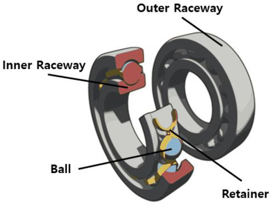
Figure 1.
Components of rolling bearing.
2.2. Denoising Autoencoder (DAE)
The autoencoder (AE), one of the most representative unsupervised learning methods in deep learning, was proposed by Hinton et al. [28]. An autoencoder is composed of an encoder and a decoder. The encoder extracts the important functions hidden in the input data in a compressed form, and the decoder recovers it based on the compressed data from the encoder. In general, as the number of neurons in the hidden layer that extracts important features is smaller than the input, data can be compressed [29]. The DAE is a slight modification of the basic AE learning method to further strengthen the restoration process [30]. The DAE is an AE with the purpose of minimizing errors by comparing the training results with existing data; this takes place by placing the noisy training data into the encoder. Figure 2 shows the structure of the DAE. First, X’ is created by adding noise to the existing image X. X’ with added noise is used as the input to the DAE, and the output Z is trained to be close to the image X.
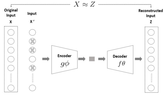
Figure 2.
Structure of the denoising autoencoder.
2.3. Convolution Neural Network (CNN)
CNNs are among the neural networks frequently used for image processing in deep learning [31,32,33]. CNNs are networks in which information is not periodic and flows in one direction. As shown in Figure 3, it can be divided into a part that extracts features of an image and a part that classifies the class. The feature extraction area is composed of a convolutional layer and a pooling layer in a stacked multiple shape. The convolutional layer is an element that reflects the activation function after applying a filter to the input data. After the convolutional layer, a fully connected layer is added, and the overall CNN model is composed. As described above, the CNN consists of three layers. Each layer is described as follows.
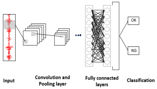
Figure 3.
Structure of the convolution neural network.
The convolutional layer serves to extract features from the data as described above. The convolutional layer includes a filter that extracts features and consists of an activation function that changes the value of this filter to a nonlinear value [34]. The output of the convolutional layer can be expressed as a mathematical equation as follows.
Normally, the convolutional layer is the layer, the feature maps are of the layer, and is the kernel. The output characteristic map in the layer is generated through the activation function . Here, represents the hidden layer, which is the basic input of . stands for bias. As passes through the entire image, it creates a feature map.
The pooling layer receives the output data of the convolutional layer as input and is used to reduce the size of the output data or to emphasize specific data [35]. In general, the pooling size and stride are set to the same size so that all elements are processed once. Methods of the processing the pooling layer include Max Pooling, Average Pooling, and Min Pooling. The pooling layer can be defined as follows.
Like the convolutional layer, stands for bias. Here, represents the sub-sampling function.
A fully connected layer is a state in which all neurons in one layer are connected to all neurons in the next layer [36]. That is, in the fully connected layer, if the i-th neuron in the n-th layer connects to the i-th neuron in the n + 1 layer, all of them are connected. This layer is used to convert the output of a two-dimensional shape into a one-dimensional array and to classify an image through a flattened matrix in the form of a one-dimensional array. The purpose of the fully connected layer is to collect all the features of the previous layer and to classify the classes to which specific data belong.
2.4. Multi-Scale Convolution Neural Network (MS-CNN)
A CNN is an optimized algorithm that can extract and classify features by receiving information from raw data. However, if there is insufficient data or insufficient information with distinct characteristics in the raw data, poor results can be obtained, regardless of the hyperparameter change. In addition, small kernels can indeed capture high-frequency features (samples close together), while large kernels can capture low-frequency features (samples covering larger regions of the observation window).
Many studies have been conducted to solve this problem. Among them, the MS-CNN has a learning model in which several convolutional layers are stacked to improve the detection performance compared to the general CNN described above [37,38]. Figure 4 shows the architecture of a MS-CNN.
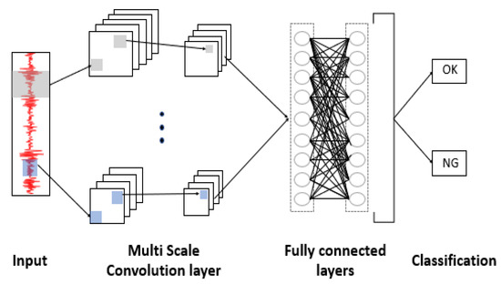
Figure 4.
Structure of a multi-scale convolution neural network.
2.5. Long Short-Term Memory (LSTM)
Using an RNN, one can effectively model time series data [39,40]. However, there is a limitation with RNNs, and long short-term memory (LSTM), developed to compensate for the shortcomings of the RNN, solves the vanishing gradient problem of the RNN [41,42]. Compared to an RNN, LSTM has an additional gate called the forgetting gate. It is impossible for existing RNNs to learn from the distant past, but LSTM can learn events from the distant past and can handle not only high-frequency signals but also low-frequency signals. This advantage of LSTM is that it shows good performance in processing time series data. The general structure of LSTM is as follows.
where is a vector input to the current time point , is the weight connecting the input to the LSTM cell, is the weight connecting the previous memory cell state and the LSTM cell, P is the diagonal peephole weight matrices, T represents tanh nonlinearities, and b is bias.
3. MS-CRNN for DAE-Based Noise Removal and Fault Detection
This section shows the DAE + MS-CRNN architecture for fault detection in a noisy manufacturing environment. The noisy data are removed through the DAE and then fed into the MS-CRNN to detect the defect.
3.1. DAE for Denoising
Deep learning training requires enough data and data reliability. This is because training results can vary depending on the amount and quality of the data. However, most of the data extracted from the field can contain outliers or corrupt values that degrade the dataset. To resolve this issue, one needs to pre-process the data. Among the many preprocessing methods, we used the DAE algorithm to remove noise. Table 1 summarizes the architecture of the DAE used in the paper.

Table 1.
DAE architecture summary.
The size of the input data was 20 × 20. The reason the input data were set as this was as follows: The vibration data to be input were vibration data with a size of 1 × 400 when viewed in one dimension. When this data were converted to two dimensions, it was set to 20 × 20 to include all vibration signals. The feature map was identified through the convolutional kernel; for pooling, max pooling was used; Relu was used as the activation function, and Adam was used as the optimization function. The final output was of size 20 × 20, the same as that of the input. Figure 5 shows the data with noise removed by the DAE in two dimensions. As shown in the figure, compared to the original data, one can see that the noise-removed data through the DAE expressed the characteristics of the original image well.
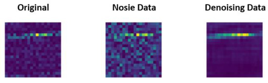
Figure 5.
Original data, data with noise added, and data with noise removed.
3.2. MS-CRNN for Bearing Fault Detection
For the detection of defects, this paper proposes the MS-CRNN. The data extracted through the DAE arrives as input to the MS-CRNN in two dimensions. The input data are input to three convolutional layers, and each layer has a different convolutional kernel. Data features are extracted through each convolutional layer. Particularly, a small-sized convolutional kernel detects a high-frequency feature, and a large-sized kernel detects a low-frequency feature. This allows more robust features to be extracted and provides both low- and high-frequency information of the existing signal. Thereafter, it is connected and input to the LSTM layer to consider the time series characteristics. After passing through LSTM, the data are entered into a fully connected layer for classification. The architecture of the proposed DAE + MS-CRNN is shown in Figure 6.
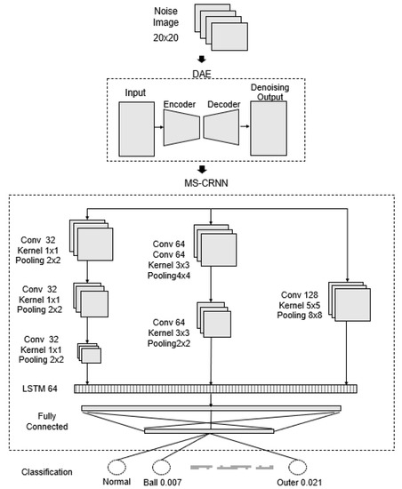
Figure 6.
Architecture of the DAE + MS-CRNN.
Data that have been denoised through the DAE were of size 20 × 20. The input data were fed into a layer with three differently sized convolution kernels. The first convolutional layer had a 1 × 1 convolutional kernel and underwent a total of three pooling processes. The second convolutional layer had a 3 × 3 convolutional kernel and went through a total of two pooling processes. The third convolutional layer had a 5 × 5 convolutional kernel and underwent a total of one pooling operation. As the first layer had a small kernel size, high-frequency features could be extracted, and in the second layer, low-frequency features and high-frequency features could be appropriately extracted. The third layer could extract features of a low-frequency region.
Max pooling was used for pooling, and Relu was used as an activation function. Thereafter, the features extracted through combining were fed as input to the LSTM layer. At this time, data were input in a one-dimensional form, and the temporal characteristics could be grasped with the long/short-term memory of LSTM. The input data were passed through the LSTM and then to the fully connected layer for classification. The input data were finally classified through the Softmax activation function. Table 2 lists the overall architecture summary of DAE + MS-CRNN.
Table 2.
Summary of the MS-CRNN architecture.
4. Experiment and Result Analysis
In this section, we describe the selection of an evaluation indicator to evaluate the proposed model and to conduct the experiment. Then, we discuss the results.
4.1. Experiment Environment
The hardware used in this study consisted of a computer with an Intel Core i7-8700K processor, GTX 1080 Ti, and 12 GB RAM. Therefore, it was possible to reduce the training time and improve the performance, unlike the capabilities of previous equipment. The result of the algorithm may vary depending on the environment of the experiment. The system specifications used for the experiments are listed in Table 3.
Table 3.
System specifications.
4.2. Evaluation Metrics
The receiver-operating characteristic curve (ROC curve), Matthews correlation coefficient (MCC), accuracy, and F1-score were calculated to evaluate the performance of the classifier for bearing defects in noisy situations.
The Matthews correlation coefficient (MCC) is used in machine learning as a measure of the quality of binary and multiclass classifications. It takes into account true and false positives and negatives and it is generally regarded as a balanced measure, which can be used even if the classes are of very different sizes. The Matthews correlation coefficient equation is:
The ROC curve is a widely used method of determining the effectiveness of a diagnostic method, and it represents the relationship between sensitivity and specificity on a two-dimensional plane. The larger the area under the ROC curve, the better the model. Sensitivity and specificity can be expressed by the following equation.
Specificity is the rate at which the model recognizes false as false. The equation is as follows:
Recall is the proportion of the true class to what the model predicts as true. The parameters, recall and precision, have a trade-off. Recall, also called sensitivity, can be expressed as follows:
Precision is the ratio of the true class to what the model classifies as true. The equation is as follows:
Accuracy is the most intuitive indicator. However, the problem is that unbalanced data labels can skew the performance. The equation for this parameter is the following:
The F1-score is called the harmonic mean, and if data labels are unbalanced, it can accurately assess the performance of the model. The equation is given as follows:
4.3. Experiment and Result
The bearing data from the CWRU dataset were used [43]. Defects ranging from 0.007 to 0.021 inches (0.0178 to 0.0533 cm) in diameter were seen in the inner orbit, the rolling element (i.e., the ball), and the outer orbit. Vibration data were recorded for motor loads of 0–3 Horsepower (motor speed 1797 to 1720 RPM). The fault test bench is illustrated in Figure 7.
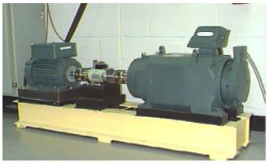
Figure 7.
Bearing simulator of CWRU.
The bearing data collected from the simulator had a total of 10 states depending on the type of defect. Each state had 1200 samples and a total of 10 states; therefore, there were 12,000 data samples. Gaussian random noise was added to the total data set, because the factory bearing signal had a lot of noise. However, in the case of CWRU data, it was determined that the noise from the field was not collected. Thus, Gaussian random noise was added to make the form of CWRU data similar to that of the data extracted from the field. This addition is thought to add at least the loud and small noises extracted from the field to the dataset we used, even indirectly. When conducting the experiment, 60% of the total data were divided into training data, 20% validation data, and 20% test data. A detailed description of the data is provided in Table 4.
Table 4.
Description of CWRU data.
To evaluate the performance of the proposed model, we evaluated it using 1D-CNN, MS-CNN, CNN-LSTM, and MS-CRNN algorithms. Each experiment showed a result of 50 epoch and was repeated more than 10 times. All experiments used the most important accuracy mentioned in the evaluation indicator, and the F-1 score was used to compensate for the shortcomings in accuracy. For an accurate experiment, a total of three experiments were conducted.
First, an experiment with the original CWRU data was conducted to evaluate the data set without additional noise. The results are shown in Table 5 and Figure 8.
Table 5.
Results of the experiment in original CWRU data condition.
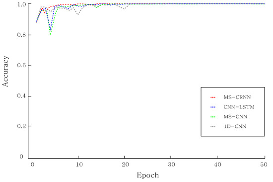
Figure 8.
Plot of the experimental results obtained for the original CWRU data state.
As a result of the experiment, it can be seen that the accuracy of all algorithms was over 99%. However, faster than other algorithms, MS-CRNN reached 100% accuracy. This would be unrealistic, because, in the case of CWRU data, most defects were well categorized because the data were extracted in a clean environment. As a result, it would be impractical to classify defects using the original CWRU data. Therefore, in this paper, an experiment was conducted by adding noise in order to create data of an environment similar to that of the field.
Second, to check the performance of MS-CRNN, we evaluated it using 1D-CNN, MS-CNN, CNN-LSTM, and MS-CRNN algorithms in the presence of noise. Table 6 shows the results of the comparison.
Table 6.
Results of the experiment under noisy conditions.
All algorithms had low accuracies when classifying defects in bearing data in noisy situations. However, it can be seen that the performance of the proposed algorithm was higher than those of other algorithms. Figure 9 shows a graph that visualizes the accuracy curves for each model. As is evident from the graph, the accuracy of the proposed model increased rapidly.
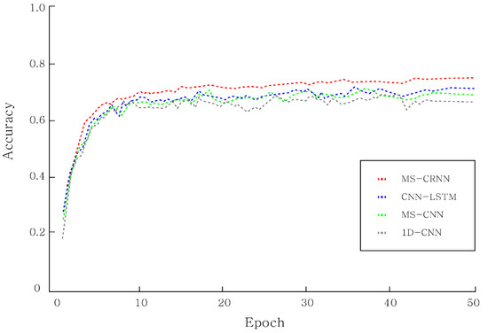
Figure 9.
Plot of the experimental results obtained for the noisy state.
Subsequently, in situations where the noise was removed using the DAE, the evaluation was conducted using 1D-CNN, MS-CNN, CNN-LSTM, and MS-CRNN. The experiment was conducted with the foregoing epoch.
As listed in Table 7, the proposed model showed an average accuracy of more than 90%, and it can be seen that the accuracy of the entire algorithm increased when the problem was solved using the DAE. In addition, we see that the proposed model had a higher accuracy than the other models did.
Table 7.
Results of the experiment under the denoising condition.
The MCC was then calculated to measure the model’s ability to classify classes. The MCC had a correlation coefficient value between −1 and +1. The closer it is to +1, the closer to a perfect prediction is made, and the closer it is to −1, the closer to the reverse prediction is made. As shown in Table 8, the proposed model showed a value close to +1 compared to other models.
Table 8.
Results of the MCC under the denoising condition.
Figure 10 shows a graph that visualizes the accuracy curve of each model when the noise was removed using the DAE. As shown by the graph, the proposed model was observed to have a high accuracy compared to the other models.
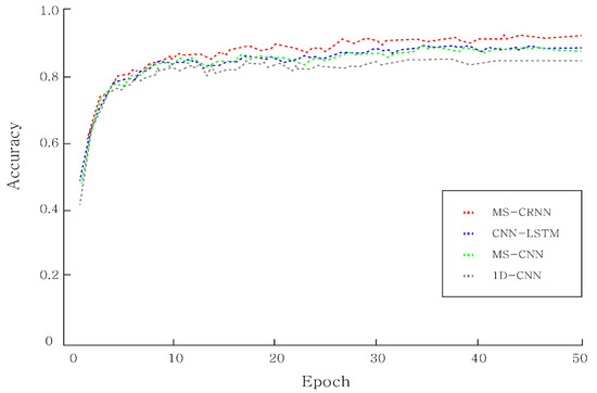
Figure 10.
Results of the experiment in the denoising state.
Figure 11 shows the results of the confusion matrix for the proposed model. By removing the noise and classifying the defect, we see that most of the time, we classified the defect with a high probability. However, as shown in Figure 10, even when the noise was removed through the DAE and the experiment was conducted, all defects could not be classified well.
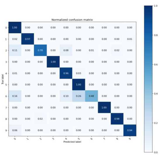
Figure 11.
Confusion matrix of the proposed DAE + MS-CRNN model.
Figure 12 shows the evaluation of the model using the ROC curve. Each class of the ROC curve was the same as that of Class Num in Table 3. The closer the ROC curve area is to a value of 1, the better the model performance. As is evident from the ROC curve, we achieved an area of 0.9 or more in most classes.
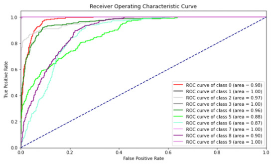
Figure 12.
ROC curve of the proposed DAE + MS-CRNN model.
5. Conclusions
The early detection of bearing defects plays an important role in identifying failures in the equipment in which the bearings are installed. In this paper, we showed a better approach to classifying defects in bearings provided by CWRU.
CWRU data differ a lot from data collected in the actual field. They do not contain other mechanical elements and they have less noise compared to field data. This paper changed the data using Gaussian random noise to make the CWRU data as close as possible to the actual field data.
In this study, a dataset similar to a noisy manufacturing environment was created for application to the actual site. Using this, we proposed the DAE algorithm to pre-process the bearing data and we proposed the optimal algorithm MS-CRNN to classify the vibration signal of the bearing. The proposed method was more realistic and performed better than the approaches in previous studies. In addition, it can be said that it is an algorithm that can be applied in the field because the problem was solved with its application in consideration of the field situation when compared with other studies. However, the proposed method had limitations. First, it did not detect any subdivided defects. The CWRU data set used in our paper was largely specialized in ball defects, inner race, and outer race, and other defects could not be found. Second, the noise could not be completely removed. In the case of the proposed DAE, it did not completely remove noise, so a more effective noise reduction method would be needed.
In future work, we will study a method to detect defects based on bearing data provided from equipment equipped with actual bearings. We will also study how to classify and, in consideration of mechanical factors, detect defects by further subdividing each type of defect. In addition, in the case of the proposed DAE, as the noise cannot be completely removed, we will work on a better noise removal method.
Author Contributions
Conceptualization, S.O. and J.J.; methodology, S.O. and S.H.; software, S.O.; validation, S.O. and J.J.; formal analysis, S.O. and S.H.; investigation, S.O.; resources, J.J.; data curation, S.O.; writing—original draft preparation, S.O.; writing—review and editing, J.J. and S.H.; visualization, S.O.; supervision, J.J.; project administration, J.J.; funding acquisition, J.J. All authors have read and agreed to the published version of the manuscript.
Funding
This research was supported by the MSIT (Ministry of Science and ICT), Korea, under the ITRC (Information Technology Research Center) support program (IITP-2021-2018-0-01417) supervised by the IITP (Institute for Information & Communications Technology Planning & Evaluation) and the Smart Factory Technological R&D Program S2727186 funded by Ministry of SMEs and Startups(MSS, Korea).
Institutional Review Board Statement
Not applicable.
Informed Consent Statement
Not applicable.
Data Availability Statement
Publicly available datasets were analyzed in this study. This data can be found here: [https://csegroups.case.edu/bearingdatacenter/pages/welcome-case-western-reserve-university-bearing-data-center-website] (accessed on 28 October 2016).
Acknowledgments
This work was supported by the Smart Factory Technological R&D Program S2727115 funded by Ministry of SMEs and Startups (MSS, Korea).
Conflicts of Interest
The authors declare no conflict of interest.
References
- Dombrowski, U.; Wagner, T. Mental strain as field of action in the 4th industrial revolution. Procedia CIRP 2014, 17, 100–105. [Google Scholar] [CrossRef]
- Abramovici, M.; Göbel, J.C.; Neges, M. Smart engineering as enabler for the 4th industrial revolution. In Integrated Systems: Innovations and Applications; Springer: Cham, Switzerland, 2015; pp. 163–170. [Google Scholar]
- Nelson Raja, P.; Kannan, S.M.; Jeyabalan, V. Overall line effectiveness—A performance evaluation index of a manufacturing system. Int. J. Product. Qual. Manag. 2010, 5, 38–59. [Google Scholar] [CrossRef]
- Hashemian, H.M. State-of-the-art predictive maintenance techniques. IEEE Trans. Instrum. Meas. 2010, 60, 226–236. [Google Scholar] [CrossRef]
- Selcuk, S. Predictive maintenance, its implementation and latest trends. Proc. Inst. Mech. Eng. Part B J. Eng. Manuf. 2017, 231, 1670–1679. [Google Scholar] [CrossRef]
- Kotzalas, M.N.; Harris, T.A. Fatigue failure progression in ball bearings. J. Trib. 2001, 123, 238–242. [Google Scholar] [CrossRef]
- El Laithy, M.; Wang, L.; Harvey, T.J.; Vierneusel, B.; Correns, M.; Blass, T. Further understanding of rolling contact fatigue in rolling element bearings—A review. Tribol. Int. 2019, 140, 105849. [Google Scholar] [CrossRef]
- Zarei, J.; Poshtan, J. Bearing fault detection using wavelet packet transform of induction motor stator current. Tribol. Int. 2007, 40, 763–769. [Google Scholar] [CrossRef]
- Cerrada, M.; Sánchez, R.V.; Li, C.; Pacheco, F.; Cabrera, D.; de Oliveira, J.V.; Vásquez, R.E. A review on data-driven fault severity assessment in rolling bearings. Mech. Syst. Signal Process. 2018, 99, 169–196. [Google Scholar] [CrossRef]
- Liu, H.; Zhou, J.; Zheng, Y.; Jiang, W.; Zhang, Y. Fault diagnosis of rolling bearings with recurrent neural network-based autoencoders. ISA Trans. 2018, 77, 167–178. [Google Scholar] [CrossRef] [PubMed]
- Duan, Z.; Wu, T.; Guo, S.; Shao, T.; Malekian, R.; Li, Z. Development and trend of condition monitoring and fault diagnosis of multi-sensors information fusion for rolling bearings: A review. Int. J. Adv. Manuf. Technol. 2018, 96, 803–819. [Google Scholar] [CrossRef]
- Sun, M.; Wang, H.; Liu, P.; Huang, S.; Fan, P. A sparse stacked denoising autoencoder with optimized transfer learning applied to the fault diagnosis of rolling bearings. Measurement 2019, 146, 305–314. [Google Scholar] [CrossRef]
- Xu, Y.; Li, Z.; Wang, S.; Li, W.; Sarkodie-Gyan, T.; Feng, S. A hybrid deep-learning model for fault diagnosis of rolling bearings. Measurement 2021, 169, 108502. [Google Scholar] [CrossRef]
- Zheng, J.; Pan, H.; Cheng, J. Rolling bearing fault detection and diagnosis based on composite multiscale fuzzy entropy and ensemble support vector machines. Mech. Syst. Signal Process. 2017, 85, 746–759. [Google Scholar] [CrossRef]
- Zhao, D.; Gelman, L.; Chu, F.; Ball, A. Novel method for vibration sensor-based instantaneous defect frequency estimation for rolling bearings under non-stationary conditions. Sensors 2020, 20, 5201. [Google Scholar] [CrossRef]
- Song, L.; Wang, H.; Chen, P. Vibration-based intelligent fault diagnosis for roller bearings in low-speed rotating machinery. IEEE Trans. Instrum. Meas. 2018, 67, 1887–1899. [Google Scholar] [CrossRef]
- Hao, Y.; Song, L.; Cui, L.; Wang, H. A three-dimensional geometric features-based SCA algorithm for compound faults diagnosis. Measurement 2019, 134, 480–491. [Google Scholar] [CrossRef]
- Shi, H.T.; Bai, X.T.; Zhang, K.; Wu, Y.H.; Yue, G.D. Influence of uneven loading condition on the sound radiation of starved lubricated full ceramic ball bearings. J. Sound Vib. 2019, 461, 114910. [Google Scholar] [CrossRef]
- Neupane, D.; Seok, J. Bearing Fault Detection and Diagnosis Using Case Western Reserve University Dataset with Deep Learning Approaches: A Review. IEEE Access 2020, 8, 93155–93178. [Google Scholar] [CrossRef]
- Zhang, H.; Chen, X.; Zhang, X.; Ye, B.; Wang, X. Aero-engine bearing fault detection: A clustering low-rank approach. Mech. Syst. Signal Process. 2020, 138, 106529. [Google Scholar] [CrossRef]
- Nivesrangsan, P.; Jantarajirojkul, D. Bearing fault monitoring by comparison with main bearing frequency components using vibration signal. In Proceedings of the 2018 5th International Conference on Business and Industrial Research (ICBIR), Bangkok, Thailand, 17–18 May 2018; IEEE: Piscataway, NJ, USA, 2018; pp. 292–296. [Google Scholar]
- Ozcan, I.H.; Eren, L.; Ince, T.; Bilir, B.; Askar, M. Comparison of time-domain and time-scale data in bearing fault detection. In Proceedings of the 2019 International Aegean Conference on Electrical Machines and Power Electronics (ACEMP) & 2019 International Conference on Optimization of Electrical and Electronic Equipment (OPTIM), Istanbul, Turkey, 27–29 August 2019; IEEE: Piscataway, NJ, USA, 2019; pp. 143–146. [Google Scholar]
- Shijie, S.; Kai, W.; Xuliang, Q.; Dan, Z.; Xueqing, D.; Jiale, S. Investigation on Bearing Weak Fault Diagnosis under Colored Noise. In Proceedings of the 2020 Chinese Control and Decision Conference (CCDC), Hefei, China, 22–24 August 2020; IEEE: Piscataway, NJ, USA, 2020; pp. 5097–5101. [Google Scholar]
- Shi, H.; Guo, L.; Tan, S.; Bai, X. Rolling bearing initial fault detection using long short-term memory recurrent network. IEEE Access 2019, 7, 171559–171569. [Google Scholar] [CrossRef]
- Li, C.; Zhang, W.E.I.; Peng, G.; Liu, S. Bearing fault diagnosis using fully-connected winner-take-all autoencoder. IEEE Access 2017, 6, 6103–6115. [Google Scholar] [CrossRef]
- Zhang, W.; Li, C.; Peng, G.; Chen, Y.; Zhang, Z. A deep convolutional neural network with new training methods for bearing fault diagnosis under noisy environment and different working load. Mech. Syst. Signal Process. 2018, 100, 439–453. [Google Scholar] [CrossRef]
- Mayes, I.W.; Davies, W.G.R. Analysis of the Response of a Multi-Rotor-Bearing System Containing a Transverse Crack in a Rotor. J. Vib. Acoust. Stress Reliab. 1984, 106, 139–145. [Google Scholar] [CrossRef]
- Hinton, G.E.; Salakhutdinov, R.R. Reducing the dimensionality of data with neural networks. Science 2006, 313, 504–507. [Google Scholar] [CrossRef] [PubMed]
- Fournier, Q.; Aloise, D. Empirical comparison between autoencoders and traditional dimensionality reduction methods. In Proceedings of the 2019 IEEE Second International Conference on Artificial Intelligence and Knowledge Engineering (AIKE), Sardinia, Italy, 3–5 June 2019; IEEE: Piscataway, NJ, USA, 2019; pp. 211–214. [Google Scholar]
- Majeed, S.; Mansoor, Y.; Qabil, S.; Majeed, F.; Khan, B. Comparative analysis of the denoising effect of unstructured vs. convolutional autoencoders. In Proceedings of the 2020 International Conference on Emerging Trends in Smart Technologies (ICETST), Karachi, Pakistan, 26–27 March 2020; IEEE: Piscataway, NJ, USA, 2020; pp. 1–5. [Google Scholar]
- Lo, S.C.B.; Chan, H.P.; Lin, J.S.; Li, H.; Freedman, M.T.; Mun, S.K. Artificial convolution neural network for medical image pattern recognition. Neural Netw. 1995, 8, 1201–1214. [Google Scholar] [CrossRef]
- Mishkin, D.; Sergievskiy, N.; Matas, J. Systematic evaluation of convolution neural network advances on the imagenet. Comput. Vis. Image Underst. 2017, 161, 11–19. [Google Scholar] [CrossRef]
- Guo, X.; Chen, L.; Shen, C. Hierarchical adaptive deep convolution neural network and its application to bearing fault diagnosis. Measurement 2016, 93, 490–502. [Google Scholar] [CrossRef]
- Liu, T.; Fang, S.; Zhao, Y.; Wang, P.; Zhang, J. Implementation of training convolutional neural networks. arXiv 2015, arXiv:1506.01195. [Google Scholar]
- Yu, D.; Wang, H.; Chen, P.; Wei, Z. Mixed pooling for convolutional neural networks. In International Conference on Rough Sets and Knowledge Technology; Springer: Cham, Switzerland, 2014; pp. 364–375. [Google Scholar]
- Traore, B.B.; Kamsu-Foguem, B.; Tangara, F. Deep convolution neural network for image recognition. Ecol. Inform. 2018, 48, 257–268. [Google Scholar] [CrossRef]
- Li, G.; Yu, Y. Visual saliency detection based on multiscale deep CNN features. IEEE Trans. Image Process. 2016, 25, 5012–5024. [Google Scholar] [CrossRef]
- Wang, J.; Zhuang, J.; Duan, L.; Cheng, W. A multi-scale convolution neural network for featureless fault diagnosis. In 2016 International Symposium on Flexible Automation (ISFA); IEEE: Piscataway, NJ, USA, 2016; pp. 65–70. [Google Scholar]
- Koutnik, J.; Greff, K.; Gomez, F.; Schmidhuber, J. A clockwork rnn. In Proceedings of the 31st International Conference on Machine Learning, Beijing, China, 21–26 June 2014; PMLR: New York, NY, USA, 2014; pp. 1863–1871. [Google Scholar]
- Williams, G.; Baxter, R.; He, H.; Hawkins, S.; Gu, L. A comparative study of RNN for outlier detection in data mining. In Proceedings of the 2002 IEEE International Conference on Data Mining, Maebashi City, Japan, 9–12 December 2002; IEEE: Piscataway, NJ, USA, 2002; pp. 709–712. [Google Scholar]
- Gers, F.A.; Schmidhuber, J.; Cummins, F. Learning to Forget: Continual Prediction with LSTM. In Proceedings of the 9th International Conference on Artificial Neural Networks: ICANN’99, Edinburgh, UK, 7–10 September 1999; pp. 850–855. [Google Scholar]
- Greff, K.; Srivastava, R.K.; Koutník, J.; Steunebrink, B.R.; Schmidhuber, J. LSTM: A search space odyssey. In IEEE Transactions on Neural Networks and Learning Systems; IEEE: Piscataway, NJ, USA, 2016; Volume 28, pp. 2222–2232. [Google Scholar]
- Bearing Data Center Seeded Fault Test Data. Available online: https://csegroups.case.edu/bearingdatacenter/pages/welcome-case-western-reserve-university-bearing-data-center-website (accessed on 28 October 2016).
Publisher’s Note: MDPI stays neutral with regard to jurisdictional claims in published maps and institutional affiliations. |
© 2021 by the authors. Licensee MDPI, Basel, Switzerland. This article is an open access article distributed under the terms and conditions of the Creative Commons Attribution (CC BY) license (https://creativecommons.org/licenses/by/4.0/).