Article

Classification Performance of Thresholding Methods in the Mahalanobis–Taguchi System

1
Razak Faculty of Technology and Informatics, Universiti Teknologi Malaysia, Jalan Sultan Yahya Petra, Kuala Lumpur 54100, Malaysia
2
Institute of Engineering Mathematics, Faculty of Applied and Human Sciences, Universiti Malaysia Perlis (UniMAP), Arau 02600, Malaysia
3
Putrajaya Campus, Universiti Tenaga Nasional (UNITEN), Jalan IKRAM-UNITEN, Kajang 43000, Malaysia
4
Faculty of Manufacturing and Mechatronic Engineering Technology, Universiti Malaysia Pahang, Pekan 26600, Malaysia
*
Author to whom correspondence should be addressed.
Appl. Sci. 2021, 11(9), 3906; https://doi.org/10.3390/app11093906
Submission received: 7 April 2021 / Revised: 22 April 2021 / Accepted: 22 April 2021 / Published: 26 April 2021
(This article belongs to the Topic Interdisciplinary Studies for Sustainable Mining)

Abstract

:
The Mahalanobis–Taguchi System (MTS) is a pattern recognition tool employing Mahalanobis Distance (MD) and Taguchi Robust Engineering philosophy to explore and exploit data in multidimensional systems. The MD metric provides a measurement scale to classify classes of samples (Abnormal vs. Normal) and gives an approach to measuring the level of severity between classes. An accurate classification result depends on a threshold value or a cut-off MD value that can effectively separate the two classes. Obtaining a reliable threshold value is very crucial. An inaccurate threshold value could lead to misclassification and eventually resulting in a misjudgment decision which in some cases caused fatal consequences. Thus, this paper compares the performance of the four most common thresholding methods reported in the literature in minimizing the misclassification problem of the MTS namely the Type I–Type II error method, the Probabilistic thresholding method, Receiver Operating Characteristics (ROC) curve method and the Box–Cox transformation method. The motivation of this work is to find the most appropriate thresholding method to be utilized in MTS methodology among the four common methods. The traditional way to obtain a threshold value in MTS is using Taguchi’s Quadratic Loss Function in which the threshold is obtained by minimizing the costs associated with misclassification decision. However, obtaining cost-related data is not easy since monetary related information is considered confidential in many cases. In this study, a total of 20 different datasets were used to evaluate the classification performances of the four different thresholding methods based on classification accuracy. The result indicates that none of the four thresholding methods outperformed one over the others in (if it is not for all) most of the datasets. Nevertheless, the study recommends the use of the Type I–Type II error method due to its less computational complexity as compared to the other three thresholding methods.

1. Introduction

The Mahalanobis–Taguchi System (MTS) is a pattern information technology that aids the quantitative decision-making process by constructing a multivariate measurement scale using data analytic methods [1]. It was developed by the renowned Japanese Quality guru Dr. Genichi Taguchi. The MTS methodology started with the theory of Mahalanobis distance (MD) formulated by the famous Indian statistician, Dr. P.C. Mahalanobis in 1936 [2] inspired by his determination to examine if the Indian people who married European people came from specific caste levels. The formulation of MD was then extended by Dr. Taguchi who integrated the MD formulation with his robust engineering concepts to enhance the MD methodology to become a popular application tool for pattern recognition and forecasting technique in multidimensional systems [3]. Therefore, numerous applications of MTS ranging to the fields of remanufacturing, medical diagnosis, pattern recognition, aerospace, agro-cultures, administration, banking and finances have been reported [3,4,5,6,7]. One of the prominent functions of MTS is to classify two groups of samples such as classifying groups of healthy and unhealthy patients, conformance and nonconformance products, normal and abnormal state of conditions, acceptable and non-acceptable of approval terms as well as other binary discrimination purposes. In MTS, to classify any two or more samples among the sample groups, MD values for each sample are calculated based on their common feature datasets. The MD values computed are viewed as points in the high dimensional space and they represent the distances of the corresponding samples from each in a univariate scale. If the MD values between the two recognition samples are “closer”, then the two samples could be said to have a common similarity otherwise, they are different from each other. Then, the question arises as to how close is “closer” as mentioned previously. This is where a threshold value or a cut-off value is required to carrying out the classification process effectively.
In the MTS context, Taguchi proposed the use of Taguchi’s Quadratic Loss Function (QLF) as the mean to determine a threshold value to classify samples [8]. QLF aims to minimize the monetary loss resulted from wrongly classify the samples (false alarm). Thus, cost information associated with the misclassification problems is required to determine the threshold value. The next section will discuss the fundamental concept of QLF in further detail. However, QLF was seen as impractical because of the difficulty in estimating the relative cost or the monetary loss in each sample case [9,10,11]. Therefore, several state-of-the-arts thresholding methods have been reported in the literature as the alternative ways to determine the threshold in the MTS methodology. The following four thresholding methods namely probabilistic thresholding method [12,13], Type-I and Type-II errors method [14,15,16,17], ROC curve method [9,13] and control chart method via Box–Cox transformation [18] are the most common thresholding methods being deployed in the MTS which will also be discussed in further details in the next section. The aim of this study is to compare the effectiveness of these four common thresholding methods in MTS methodology. To the best of the authors’ knowledge, no comparison works have been conducted to evaluate the effectiveness of these four common thresholding methods in MTS. The reports found in the literature were mainly focused on demonstrating the usage of the threshold methods based on unique case studies of the researchers. It is therefore the motivation of this paper to compare the classification performance of these four common thresholding methods in the MTS across several datasets.
The paper is presented as follows, a theoretical overview of the fundamental concept of MD and MTS is explained in Section 2. A brief discussion on the fundamental concepts of thresholding methods used in the MTS including the Quadratic Loss Function, Probabilistic Thresholding method, Type-I and Type-II Errors method, ROC curve method and Box–Cox Transformation method are discussed in Section 3. Section 4 and Section 5 explain datasets used in the study which involved 20 datasets and the results and discussion of the comparison studies in evaluating the classification performances of the threshold methods. Section 6 concludes the key findings and contributions of this paper.

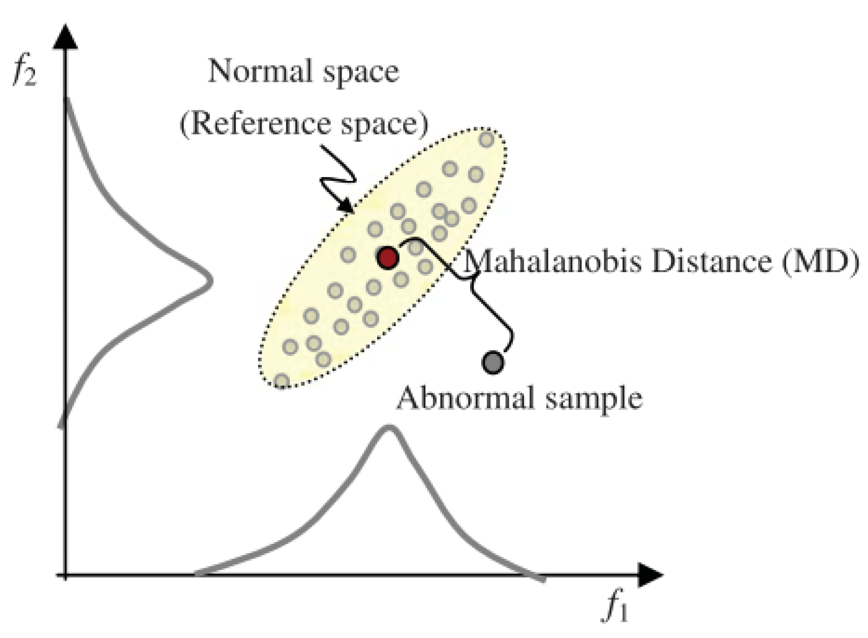
2. The Concept of Mahalanobis Distance (MD)

MD is a dimensionless distance measure based on the correlation between features and pattern differences that can be analysed with respect to a reference population [19], as shown in Figure 1. This reference population is called the normal space. The distance measure is termed the Mahalanobis Scale (MS) and aids the discriminant analysis approach by assessing the level of abnormality of datasets against the normal space.
MD has an elliptical shape (see Figure 1) due to the correlation effect between the features. If there is no correlation, the MD is the same as the Euclidean Distance (ED) that has a circular shape. MD is different from Euclidean Distance since the latter does not consider the correlation among the features of the data points.

2.1. Mahalanobis Distance (MD) Formulation

MD is defined as in Equation (1):
M D j = D j 2 = Z i j T C 1 Z i j   with   Z i j = x i j m i s i  
where;
k = the total number of features;
i = the number of features (i = 1, 2, …, k);
j = the number of samples (j = 1, 2, …, n);
Zij = the standardized vector of normalized characteristics of xij;
xij = the value of the ith characteristic in the jth observation;
mi = the mean of the ith characteristic;
si = the standard deviation of the ith characteristic;
T = the transpose of the vector;
C−1 = the inverse of the correlation coefficient matrix.
MD has been well deployed in a broad array of applications [20,21] mainly because it is very effective in tracking intervariable correlations in data.

2.2. Mahalanobis–Taguchi System (MTS) Procedures

Taguchi extended the MD methodology with his robust engineering concepts to become an efficient and effective strategy for prediction and forecasting in multidimensional systems. In the MTS methodology, the formulation of MD is “scaled” where the existing MD formulation stated in Equation (1) is divided by a term “k” that denotes the number of variables or features of a recognition system. Therefore, the equation for calculating the scaled MD in the MTS methodology becomes:
M D j =   D j 2 = 1 k Z i j T C 1 Z i j
From this point onwards, the MD computation will be based on Equation (2). The MD offers a statistical measure to diagnose unknown sample conditions with known samples and provides information to make future predictions.
The fundamental steps in the MTS methodology are explained in the next section.
STAGE 1: Construction of measurement scale
To construct a measurement scale, a homogeneous dataset from normal observations needs to be collected to build a reference group called the normal group [22]. It is used as a base or reference point in the scale. The collected normal datasets need to be standardized to obtain a dimensionless unit vector followed by the MD computation. Practically, the MD for unknown data is interpreted as the nearness to the mean of the normal group. As a countercheck, the average value of the MDs for the normal group must always be close to unity; therefore they are called the normal space or Mahalanobis Space (MS) [23].
The steps for the construction of the MS are outlined below:
Calculate the mean characteristic in the normal dataset as:
x ¯ i = j = 1 n X i j n
Then, calculate the standard deviation for each characteristic:
s i = j = 1 n ( X i j x ¯ i ) 2 n 1
Next, standardise each characteristic to form the normalized data matrix (Zij) and its transpose ( Z i j T ):
Z i j = ( X i j x ¯ i ) s i
Then, verify that the mean of the normalized data is zero:
z ¯ i = j = 1 n Z i j n = 0
Verify that the standard deviation of the normalized data is one:
s z = j = 1 n ( Z i j z ¯ i ) 2 n 1 = 1
Form the correlation coefficient matrix (C) of the normalized data. The element matrix (cij) is calculated as follows:
c i j = m = 1 n ( Z m Z j m ) n 1
Compute inverse correlation coefficient matrix (C−1)
where:
C = C o v ( X , Y ) V ( X ) V ( Y )
where:
C o v   ( X , Y ) = 1 n 1 i = 1 n ( X i X ¯ ) ( Y i Y ¯ )
  • n is the number of samples,
  • X and Y are two different features being correlated,
  • X bar and Y bar are the averages among the data in each variable, and
  • V(X) and V(Y) are the variances of X and Y.
Finally, calculate the MDj using Equation (2).
STAGE2: Assessment of the measurement scale
To evaluate the measurement scale, observations outside the MS or abnormal datasets are used. The same mathematical calculation is repeated to calculate the same goal (MD value) using the abnormal sample data. However, the abnormal data are normalized based on the mean, standard deviation and correlation matrix of the normal group. The normal MDs and abnormal MDs are then compared. An acceptable measurement scale should demonstrate significant discrimination between the normal and abnormal MD values.
STAGE 3: Identify significant features
In the third stage, the system is optimized by means of selecting only the features that are known to be significant or “useful” for the system. This is where the Orthogonal Array (OA) and signal-to-noise ratio (SNR) are utilized. The features are assigned to an orthogonal array experimental run of two-level, in which “used” is signified as level 1 and “not used” as level 2. The MD for each experiment runs for all “used” features from each abnormal sample is calculated. The calculated MD values are recorded according to the experimental run. The SNR based on the MD values for all samples is then computed.

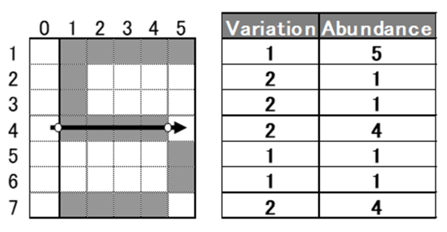
2.2.1. The Role of the Orthogonal Array (OA) in MTS

Orthogonal array (OA) is a type of fractional factorial design of experiment introduced by C.R. Rao in 1947 [24]. It is different from the traditional fractional factorial DOE in the sense that it tries to balance the combination or interaction of factors equally with the minimum number of experimental runs. In MTS, the orthogonal array structure is represented by Latin symbology as La (bc) where L is the Latin Square, a is the number of runs, b is the number of factor levels and c is the number of main factors. Table 1 illustrates an example of an OA structure for seven factors with eight runs and two factor levels.
The name “orthogonal” is suggested not because of the perpendicular attribute of the structure but rather it is defined as any pairs of columns with the same repetition number of combinations of factors [24]. To illustrate further, using the OA in Table 2 as an example, take a pair between column 1 and column 2, the repetition number of each level of combinations in this column pair is the same (which is twice in this case). The same number of repetitions should be obtained for the rest of the column pairs thus the L8 (27) array depicted by Table 1 can be said to be orthogonal. Table 2 illustrates the number of repetitions in level combination for another three more column pairs.
In MTS, OAs are used to select the features of importance by minimizing the different combinations of the original set of features. The features are assigned to the different columns of the array. Since the features have only two levels, a two-level array is used in MTS as illustrated in Table 2. For each run of an OA, MDs corresponding to the known abnormal conditions are computed. The importance of features is judged based on their ability to measure the degree of abnormality on the measurement scale [25]. This is where the signal to noise ratio metric is deployed. Further discussion on OA concepts can be found from [24,26,27,28].

2.2.2. The Role of the SNR in MTS

The signal-to-noise ratio (SNR) concept which can be considered as the core essence of Taguchi philosophy, is developed by Taguchi who get inspired when he was practicing an engineering profession in a Japanese telecommunication company in the 1950s. In the telecommunication context, the SNR captures the magnitude of true information (i.e., signals) after making some adjustments for uncontrollable variation (i.e., noise) [26]. In Taguchi’s robust engineering concept, the SNR is defined as the measure of the functionality of the system, which exploits the interaction between the control factors and the noise factors. A “gain” in the SNR value denotes a reduction in the variability, hence a reduction in the number of factors associated with the “noise” (factors that are considered insignificant for the classification effort) resulting in a reduction of the classification process in terms of time and cost. Refs. [27,28] provide a detailed description of SNR concepts and their origin of the formulation.
In the context of MTS, the SNR is defined as the measure of the accuracy of the measurement scale for predicting abnormal conditions [26]. In MTS, a higher value of SNR which is expressed in decibels (dB), means a lower prediction error. SNR is used as a metric to assess how significant each variable in the system contributes to the ability to discriminate between normal and abnormal observations. It could also be used to assess the overall performance of a given MTS model and the degree of improvement that it has made after underwent the optimization process.
The two most commonly used SNRs in MTS are larger-the-better (LTB) and dynamic [23,26,29]. In this study, the larger-the-better SNR will be utilized due to less computational complexity.

2.2.3. Larger-the-Better SNR

LTB is formulated as in Equation (11) below, where t is the abnormal conditions and D12, D22, …, Dt2 is the MDs corresponding to the abnormal situations. The SNR (for the larger-the-better criterion) corresponding to qth run of OA is given as:
S N R = η q = 10 l o g 10 [ 1 t   i = 1 t ( 1 D i 2 ) ]
For each variable Xi, SNR1 represents the average SNR of level 1 for Xi while SNR2 represents the average SNR of level 2 for Xi throughout the vertical columns of the OA. Thus, positive gains from Equation (12) constitute useful features while negative gains constitute otherwise. Table 3 illustrates the assessment made using the SNR to evaluate significant factors of the L8 OA structure.
G a i n = S N R 1 S N R 2
STAGE 4: Future deployment with significant features
The optimized system is then re-evaluated with the abnormal samples to validate the effectiveness of assessing the discriminant power. Once confirmed, the optimized system is used for future applications in diagnosis, classification, or forecasting purposes. Figure 2 illustrates the summary of the fundamental stages in MTS. Note that it is in Stage 4 where the optimum threshold value (MDT) of the optimized system is obtained prior to future diagnosis or classification usage.

3. Overview on Common Thresholding Methods in the Mahalanobis Taguchi System

3.1. Quadratic Loss Function

Quadratic Loss Function (QLF) was introduced by Dr. Genichi Taguchi which aims to quantify the quality lost to society [30]. Taguchi defines “loss to society” not only in terms of operational problems such as rejections, scraps, or rework but also in terms of among others, pollution that is added to the environment, products that are worn out too quickly while in use, or other negative effects that could occur over the operational life of the products. In the context of Robust Engineering Design, QLF is used to determine the specification limits for a product. Ref. [30] provides a clear discussion of QLF. QLF promotes that any deviation on either side of the quality target incurs a monetary loss. This concept helps management understand the importance of robustness of a design, because the variation is expressed in monetary terms.
The idea of QLF is applied in the MTS to determine the threshold values for the classification problem [8]. Take a medical diagnosis problem, for example, if the MD value of a patient’s blood sample exceeds the threshold value, the patient is classified as unhealthy, and thus leading to a decision where the patient should be given a further complete medical examination. In Quadratic Loss Function, the optimal threshold (MDT) is given by:
M D T = A A 0   D
where:
MDT = the threshold (in MD term)
A = the cost of the complete examination of patients who diagnose as unhealthy (including loss of time),
A0 = the monetary loss caused by not taking the complete examination and having the disease show up before the next examination or the loss increase after having subjective symptoms followed by taking a complete examination,
D = the mid-value of the MD of a patient group having the subjective symptoms
The key element in the QLF concept is to balance between the cost of treating a patient and the cost of not treating a patient (as in the medical application). However, in real practical applications, even outside the medical diagnosis problems, obtaining the associated monetary information was seen to be impractical and difficult to obtain [10,13,31], hence several alternative approaches to determine the optimal threshold value have been reported in the literature of which several of them are discussed as follows.

3.2. Probabilistic Thresholding Method

Ref. [13] introduced a probabilistic thresholding method (PTM) in their study to evaluate the classification performance of MTS grounded by Chebyshev’s theorem. Ref. [32] used PTM based on Chebyshev’s theorem in his work to reduce solder paste inspection process in a Surface-Mount Technology (SMT) assembly using MTS. Chebyshev’s theorem is useful to estimate the probability of getting a value that deviates from the mean by less than some degree of standard deviation, especially when the probability distribution of the dataset is unknown. The optimal threshold (MDT) can be calculated with the following formula:
M D T = M D ¯ + 1 1 + λ ω 2 ×   s M D
where:
M D ¯ is the average of the MDs of the normal group,
sMD is the standard deviation of the MDs of the normal group,
λ is a small parameter or the confidence level (typically 5% or 0.05)
ω is the percentage of the normal examples whose MDs are smaller than the minimum MD of the remainder abnormal examples and do not overlap with the abnormal MDs.
Ref. [32] provides the method to determine ω as illustrated in Figure 3 for a simple example. The 10 blue boxes represent normal samples on their MD scales while the 7 orange boxes represent abnormal samples with two boxes of respective samples being overlapped to each other. Thus, ω is obtained by taking the percentage of the non-overlapped normal boxes over the total of normal boxes which is in this case, 7 divided by 10 equivalents to 70% or 0.7 on a zero-to-one scale.

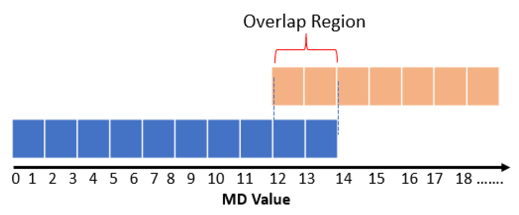
3.3. Type-I and Type-II Errors Method

Several attempts have been reported in the literature to minimize Type-I and Type-II errors in finding the optimum threshold of the MTS [14,15,18,31]. Generally, Type-I error is a misclassification error associated with the true normal samples when they were classified as abnormal while Type-II error occurred when the true abnormal samples were predicted as normal. For a two-classification problem, the normal samples can be regarded as positive, and the abnormal samples can be regarded as negative. Consequently, there will be four classification results such that:
  • TP (True Positive) = an observation is positive and predicted as positive,
  • FP (False Positive) = an observation is negative but predicted as positive,
  • TN (True Negative) = an observation is negative and predicted as negative, and
  • FN (False Negative) = an observation is positive but predicted as negative.
The four classification results could be further understood in a tabular representation as shown in Table 4 which is also known as Confusion Matrix.
Thus, from Table 4, Type-I error is derived as α = F N F N + T P while Type-II error is expressed as β = F P T N + F P . To determine the optimal threshold (MDT) is to minimize the sum of αType-I + βType-II such that:
MDT(min) = αType-I + βType-II
The optimal threshold (MDT) that minimizes the Type-I and Type-II errors could be illustrated in Figure 4:

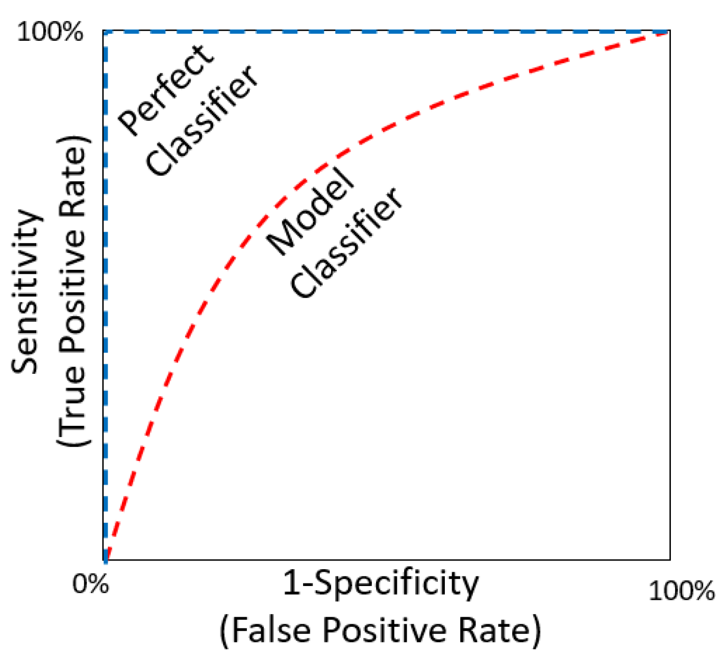
3.4. ROC Curve Method

The history of Receiver Operating Characteristics (ROC) is dated back to the World War II-era with which the radar operators used this theory to decide whether a blip on the radar receiving screen indicated an enemy battleship, a friendly allied asset, or just a “noise”. This signal detection theory was firstly popularized outside the military world by [33] in the area of phycology and over the years, the theory has been widely used in various disciplines including electronic signal detection, medical prognosis and diagnosis as well as data mining application for classification purposes [34].
In the context of the classification problem of MTS, ref. [9] deploys ROC in software defect diagnosis based on a multivariate set of software metrics and attributes by incorporating sensitivity and specificity metrics in the training dataset as the threshold value (see Figure 5). Sensitivity is defined as the proportion of actual positive class which is correctly identified as such while Specificity is the proportion of the negative class, which is correctly identified as negative such that:
S e n s i t i v i t y = T P F N + T P , S p e c i f i c i t y = T N F P + T N
Note that in Figure 5, the x-axis of the diagram uses “1-specificity” metric to denote a false positive value of the classifier. Thus, the aim is to determine the area under the curve of the model classifier of which the bigger the area the better. In other words, the closer the model classifier line (represented by the red-dotted curvy line) to the prefect classifier shape (represented by the blue-dotted line) the better chance of the model to classify all the samples correctly according to their respective classes. Thus, ref. [9] aims to find the MDT value that maximizes the area under the curve of the MTS classifier.
Using area under the ROC curve to determine a threshold value, however, could be misleading since any two ROC curves may have different shapes but they could have identical areas under the curve [35]. Thus, ref. [11] proposed instead of maximizing the area under the curve, minimizing the Euclidean Distance from any point of the classifier curve to the maximum theoretical threshold value (i.e., maximum true positive rate) is sought. Figure 6 illustrates the approach by taking the examples of an “A” as the maximum sensitivity value while points B, C, D and E represent four different points on the MTS classifier curve.
Thus, from Figure 6, the distances between the points (4 points in this example, dAB, dAC, dAD and dAE) to point A are calculated. The closer the classifier performance to point A is, the better it is. Changing the threshold will change the point coordinate on the curve. Therefore, the problem of finding the optimum threshold can be reformulated into the problem of finding the closest point that lies on the curve to point A given:
T P R = T P F N + T P , F P R = F P T N + F P
And thus, the optimum MDT is established by obtaining the shortest Euclidean Distance such that:
m i n   d A . M D T = ( F P R A F P R M D T ) 2 + ( T P R A T P R M D T ) 2 2
where dA.MDT is Euclidean Distance between point A and any point of MDT that lies on the ROC curve such as points B, C, D or E illustrated in the example of Figure 6. FPRA is the false positive rate at point A which is equal to zero. TPRA is the true positive rate at point A which is equal to one while FPRMDT is the false positive rate at the threshold MDT. TPRMDT is the true positive at threshold MDT. Thus, MDT that gives the lowest dAMDT value will be taken as the optimum threshold value (MDT).

3.5. Box–Cox Transformation

The distribution of MD values for all samples contributed to the construction of the MTS classifier does not generally follow a normal distribution. They are always skewed to the left and to the right of the MDs distribution plot since normal and abnormal samples are treated as different sample populations. Ref. [18] attempted to transformed the non-normal distribution of MDs into a normally distributed MDs distribution using Box–Cox transformation procedures. The motivation of their work comes from their intention to adopt a Control Chart Limit concept to determine the optimal MDT value. In a control limit procedure, the mean (µ) and standard deviation (σ) of the sample population in a normal distribution could be easily determined. Thus, all samples (in MD terms) are transformed using Box–Cox transformation which is defined in Equation (19)–(21) as follows:
M D i ( λ ) = 1 λ   ( M D i λ 1 ) ,   λ   0   ; i = 1 , 2 , 3 , , n M D i ( λ ) = ln ( M D i ) λ = 0   ; i = 1 , 2 , 3 . ,   n
where MDi is the MD of the ith sample, MDi(λ) is the transformed MD value. The value of λ is obtained, such that it maximizes the logarithm of the likelihood function in Equation (20) as the following:
f λ M a x ( M D , λ ) = n 2 ln [ 1 n ( ( M D i ( λ ) M D ¯ ( λ ) ) 2 ] + ( λ 1 )   i = 1 n ln ( M D i )
where, M D ¯ ( λ ) = 1 n   i = 1 n ( M D i ( λ ) ) and n is the total number of samples (both normal and abnormal).
And thus, to obtain the optimal threshold value ( τ x ) of the transformed samples, one has to minimize the following error (ε) function according to Equation (21) below:
ε ( τ ) = e 1 n h + e 2 n u
where τ is the threshold value (in Box–Cox transformed term), e1 is the number of samples classified as unhealthy (abnormal) which in fact they were healthy (normal), nh is the total number of healthy (normal) samples, e2 is the number of samples classified as healthy (normal) which in fact they were unhealthy (abnormal) while nu is the total unhealthy (abnormal) samples in the dataset.
Since τ threshold value is in the form of a transformed Box–Cox term, to convert the transformed threshold value into a non-transformed MDT form, Equation (19) is deployed by rearranging the equation into MD term by incorporating λ value which was obtained previously and accordingly.

4. Datasets

The classification performance of the four mentioned thresholding methods namely the Probabilistic Thresholding Method, the Type-I and Type-II error method, the ROC method and the Box–Cox transformation method will be tested against 20 different datasets (refer to Table 5) of which 18 of them are obtained from standard benchmark datasets based on evolutionary learning (KEEL) repository [36]. The standard benchmark datasets are originally from the UCI machine learning repository which is utilized by many for the studies of binary or two classes of classification problems (normal vs. abnormal in this case). Each sample in the datasets is randomly selected (based on their class attributes of normal or abnormal), and assigned to a Training set or a Testing set accordingly. The quantity of samples in the training and the testing set that corresponds to their class attributes is roughly divided by a 50–50 percent basis [37]. The training sets are the datasets of which the optimized number of variables (reduced variables) as well as the optimum thresholding value (MDT) are sought using the MTS procedures and the four thresholding methods respectively.
The additional two datasets namely the Medical diagnosis of liver disease [38] and the Taguchi’s charactear recognition [23] datasets are also included. The following section will briefly describe these two additional datasets.

4.1. Medical Diagnosis of Liver Disease Data

Liver disease data represent a dataset that was originally collected and used for MTS analysis by Dr. Genichi Taguchi himself during his initial work on MTS. These data can be considered as renowned data when it comes to evaluating MTS performances since it has been applied by various researchers in evaluating and analysing MTS performances in binary classification problems [23,26,30].
The story behind the data came over nearly 30 years ago when Dr. Genichi Taguchi working together with Dr. Tatsuji Kanetaka of Tokyo Tenshin Hospital on which they embarked on a joint study of liver disease diagnosis. The result of the study was made public in 1987 and the data were published in various publications as well as being used for several MTS-comparison study purposes. The data contain observations of a healthy group as well as the abnormal on 17 features as shown in Table 6.
The healthy group (MS) is constructed based on observations of 200 people (healthy), who do not have any health problems together with 17 abnormal conditions (unhealthy). These data act as the training data for the construction of Mahalanobis Space MS (reference group). While a total of 60 samples (other than the training samples) are taken as the testing samples [38].

4.2. Taguchi’s Character Recognition

It is a feature selection technique in character recognition proposed by [39] in which feature extraction of a character is based on the instances of variation and abundance items. Figure 7 illustrates an example of variation and abundance instances of a character “5”. Variation is defined as the number of switches between white-to-grey or grey-to-white as represented by the small circle; while abundance is the number of square grey boxes as the arrow passes through each row in the index (see Figure 7). These variation and abundance items act as the variables of interest in MTS for classification purposes. Ref. [23] provides a detailed explanation of these concepts and examples of how they are deployed in the MTS methodology. In this paper, pattern recognition for character “5” is selected for analysis in the study.
Ref. [23] demonstrated the use of this method in recognizing character number “5” out of several “normal” and “abnormal” samples that formed several shapes similar and not similar to a numeral “5” respectively. The data were published in 2012 which consist of 14 variables (7 abundance instances and 7 variation instances). A number of 18 normal (resemblance of character “5”) and 46 abnormal (no resemblance to numeral “5”) samples were collected for the study.

5. Results and Discussion

The optimization algorithms for all four thresholding techniques mentioned in Section 3 above were constructed using the Visual Basic language platform. The programming algorithms were then compiled on a 64-bit under high-performance computing machine with Intel Core i7-8750H Processor with DDR42666 16GB memory.

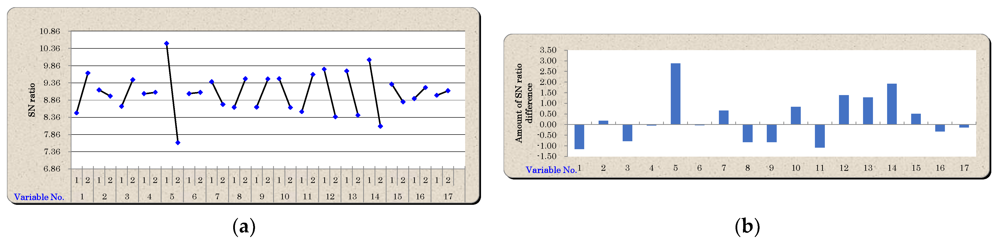
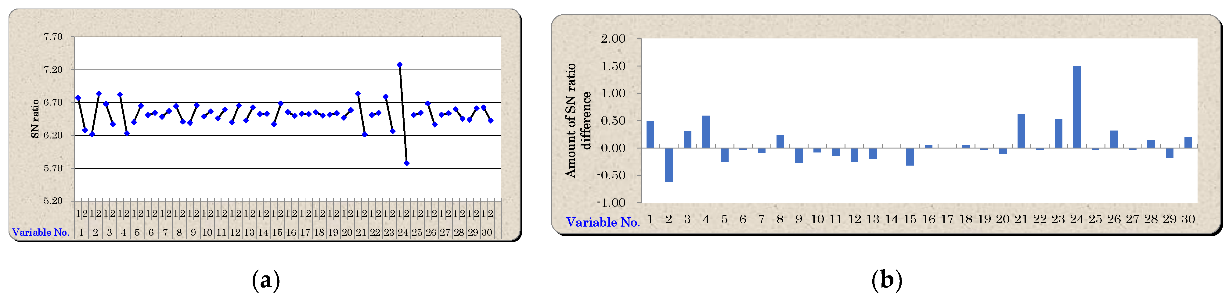
5.1. Variable Reduction Using Mahalanobis–Taguchi System

The variables of all 20 datasets were optimized using MTS procedures. Table 7 shows the optimized variables of respective datasets obtained (After Optimize) against their original variables set (Before Optimize). Note that the reduced number of variables (optimized) are the significant variables suggested by MTS for future prediction and classification purposes. Figure 8, Figure 9 and Figure 10 illustrate the optimization results based on SNR Plots and SNR Gain Charts. Due to page limitation, three datasets, namely Medical Diagnosis of Liver Disease, Wdbc and the Spambase, were displayed since these datasets showed a higher number of variable reductions as compared to the rest. The SNR Plots show the average values of SNRs based on the level of OA. The SNR Gain Charts illustrate the SNR gain between the level averages that correspond to each variable in the dataset. The positive SNR gains denote useful variables for future purposes while negative SNR gains were considered insignificant variables and thus were discarded.
Table 7 shows that more than half (>50%) of the original number of variables were removed for Wdbc, Spambase and Medical Diagnosis of liver disease datasets, while almost half (>40%) of the original variables were removed from the Appendicitis and the Coil2000 datasets. These results could significantly reduce the classification effort with a much smaller number of variables to process in those particular datasets. Unlike the rest of the datasets, the Banana, Haberman-2, Monk2, Ring and Taguchi Character Recognition datasets, however, produced no reduction in the number of variables when they were optimized using the MTS. This indicates that all original variables for these particular five datasets are found to be significant and will be fully used for future classification purposes.

5.2. Optimum Thresholds

With the optimized variables obtained via the MTS, the optimum threshold value (MDT) for each optimized dataset was computed using the four threshold methods mentioned in Section 3 previously. Table 8 tabulates the threshold values (MDT) suggested by each method of which the cut-off value to classify the testing samples (either normal or abnormal) in the testing sets will be used. Note that, the optimum λopt and the MDT in Box–Cox transformed terms are also included in the table since they are part of the items required in obtaining the optimum threshold values via Box–Cox transformation process. In this study, an MD value of a testing sample having less than or equal to MDT is denoted as normal, otherwise, it is considered abnormal.

5.3. Classification Accuracy Results

Table 9 shows the classification accuracy (in %) for each dataset based on the threshold values obtained via Type I-Type-II, ROC Curve, Chebyshev’s Theorem and Box–Cox transformation methods accordingly. The classification process is conducted using the testing sets which consist of normal and abnormal samples. These classification results will indicate how good the MDT to which the normal samples and abnormal samples in the testing sets are differentiated.
In general, the classification process is conducted firstly by computing the MD values of all samples (both normals and abnormals) in the testing set. Thus, a decision is made when the MD value of the testing sample having less than or equal to the MDT to be denoted as normal, otherwise it will be considered abnormal. These results are then compared against the true class of the samples (normal and abnormal) to which the accuracy of the classification performance is measured.
In Table 9, the classification results correspond to each dataset are shown of which bold fonts indicate superior classification performances against the others. Interestingly, it was clearly shown that none of the four thresholding methods outperformed one of the others in (if it is not for all) most of the datasets. This finding confirms the no free lunch theorem [40] in that there is no single algorithm that suits all datasets. However, an equivalent classification performance (74.21%) by all thresholding methods could be seen in the Titanic dataset. It could also be seen that Type-I–Type-II, ROC curve and the Box–Cox Transformation methods gave equivalent classification accuracies in the Appendicitis, Ionosphere and Spambase datasets as well as in the Medical Diagnosis of Liver Disease dataset of which a perfect classification performance (100%) is achieved from the three threshold methods.
Despite the complexities in computing the optimum threshold using Box–Cox transformation method, it produced nearly a perfect classification performance (98.14%) against the other three methods in the ring dataset as well as obtained equal performances with 68.49% and 96.20% accuracies in Banana and Wisconsin datasets respectively against Type-I–Type-II error. On the other hand, Type-I–Type-II error method produced a higher number of successful attempts with 11 successful frequencies over the other three methods for all datasets. Figure 11 illustrates this finding based on the results extracted from Table 8. Furthermore, the Type-I–Type-II error method seems favourable in this case since it is computationally less complex in computing the optimum threshold value as compared to the other three methods.
From Table 9, it was interesting to see that each of the thresholding methods outperformed one over the others on different datasets. For example, Chebyshev’s Theorem method outperformed the others in Bupa, Coil2000, Haberman-2, Heart, Magic, Phenome, Pima and Wdbc datasets. On the other hand, Box–Cox Transformation method seems superior on Ring and Sonar datasets while Type-I–Type-II error method was found best on Monk2 and Spectfheart. These findings indicate that the suitability and utilization of each thresholding method depend on the dataset itself. Therefore, one could conduct a trial run for all thresholding methods to come to the decision in selecting the suitable thresholding method for any dataset of interest however, it seems impractical and will increase classification efforts. Further studies should be conducted to investigate the nature and the attributes of the datasets to which thresholding methods are suitable. Perhaps a systematic procedure could be developed to guide the decision process.
Another interesting point to highlight is that out of 20 datasets, only seven of them (coil2000, Ionosphere, Ring, Spambase, Wdbc, Wisconsin, Medical Diagnosis of Liver Disease and Taguchi Character Recognition) produced classification accuracies of more than 80% across all thresholding methods by which an above 80% marks (>80%) is considered a promising prediction result [9]. The remaining datasets produced classification accuracy results with below than 80% of predictive accuracies across all thresholding methods. The lowest classification accuracy was seen on the Spectfheart dataset with a staggering low of 29.85% accuracy when predicting the testing samples based on the threshold value suggested by the ROC curve method. Generally, this not only denotes the unsuitability of the ROC method on the dataset, it also denotes that the predictive capability of the MTS seems unpromising in certain cases of datasets. This could be due to the validity of the reduced number of variables achieved during the optimization procedure of the MTS by which Orthogonal Array (OA) is utilized for feature selection. MD values is sensitive to the choices of variables in the classifier system since the computed MD value varies with different sets of significant variables. Therefore, obtaining the optimal significant variable set is crucial in the MTS particularly on the MS (the reference group).
Future studies should investigate the practicality of OA as an effective scheme for significant feature selection in the MTS. The suggestion seems to agree with reports in the literature claiming that the feature selection search mechanism using an orthogonal array (OA) for variable reduction in the MTS is inadequate and leads to inaccurate and sub-optimal solutions [41,42,43,44,45] for certain datasets. OA failed to explore other potential optimum combinations of features in their studies since the exploitation on higher-order combinations among variables in datasets using OA search structure was seen as insufficient.
The use of Swarm Intelligence-based algorithms (SI) such as the Particle Swarm Optimization (PSO), Ant Colony Optimization (ACO), Bees Algorithms (BA), Fish Algorithms (FA) to name a few, could be one alternative to handle the issue as suggested by [25]. SI-based algorithms are meta-heuristic in nature in that the search mechanism is tailored to guide a specific optimization problem heuristically toward promising solution search spaces that contain good quality solutions [46]. Further, the combination of exploration (diversification) and exploitation (intensification) search mechanism of the SI increases the ability to find optimal solutions in a reasonable time [47,48]. Hence, the strategies offered by these algorithmic techniques are worth to be explored in solving the weakness of OA in that respect. Others also suggested several alternative methods replacing the OA in MTS such as the adaptive One-Factor-at-a-Time (aOFAT) [49] and Rough-set Theory [50]. Perhaps a modification of the OA matrix structure itself with other orthogonal matrix theories such as the Paley’s cyclic matrix or Hadamard matrix [23] could possibly worth to be considered.
In MTS, Taguchi recommended using two types of signal-to-noise ratio which are “larger-the-better” and “Dynamic” signal-to-noise ratio. The former was utilized in this work. The latter type of signal-to-noise ratio (Dynamic) is another powerful selection metric that takes into account the level of abnormality of the input samples in its computational procedures. Unlike larger-the-better type signal-to-noise ratio, the Dynamic signal-to-noise ratio formulation is quite complex which makes the computational effort a challenging task however, it may provide a more promising solution. Thus, exploiting what the Dynamic signal-to-noise ratio could offer in improving the feature selection process of the MTS would be an encouraging research study in the future.
Nonetheless, this study focuses on the comparison of thresholding classification performances in the MTS between the four threshold methods mentioned previously. Based on this study, it was clearly shown that not a single threshold method produced superior classification performance for all datasets. Nevertheless, the authors seem to recommend the use of the Type-I–Type-II error method as the alternative approach as compared to the other thresholding methods owing to its simplicity with less computational burden. However, it is suggested that more studies with more datasets could be conducted in the future to strongly support this generalization.

6. Conclusions

This paper provides a comparative study to evaluate the classification performance of the MTS and to suggest the appropriate thresholding method to be utilized in MTS methodology between four common thresholding methods namely the Type-I–Type-II error method, the Probabilistic Thresholding Method, ROC curve method and the Box–Cox transformation method. To the best of the authors’ knowledge, no comparison works have been conducted to evaluate the effectiveness of those common thresholding methods towards MTS classification performances on several datasets. The outcome of this study could provide an initial insight on a general thresholding method that is suitable across several case data. The result found that none of the four thresholding methods outperformed one over the others in (if it is not for all) most of the datasets. It could also be found that the effective use of the four thresholding methods to produce promising classification performances is dataset dependant. Hence, further studies to investigate the cause of these dependency behaviours and their relationships are urged. In addition, the study also found an unpromising predictive ability of the MTS in classifying several datasets of the study. Improving the significant variable selection process of the MTS using several alternative approaches was suggested. PSO-based thresholding studies could also be considered as another thresholding alternative in improving the MTS classification problem. Nevertheless, from the study, the Type-I–Type-II error method seems favourable due to its lower algorithm complexity as compared to the other three thresholding methods. It is also recommended to evaluate the computational time complexities of these algorithms in the future to further support the findings.

Author Contributions

The lead author of this paper is F.R. Additional support was provided by W.Z.A.W.M., N.H., M.Y.A., H.Y., K.R.J. and H.H.A.T. All authors have read and agreed to the published version of the manuscript.

Funding

This work was funded by the Collaborative Research Grant Project (Project Grant No. Q.K130000.2456.08G27) under the Collaborative Research Grant Program (Program Grant No. Q.K130000.2456.08G38).

Institutional Review Board Statement

Not applicable.

Informed Consent Statement

Not applicable.

Data Availability Statement

Data are available from KEEL repository.

Acknowledgments

The authors would like to express sincere gratitude to Research Management Centre (RMC) from Universiti Teknologi Malaysia, Universiti Malaysia Perlis, Universiti Malaysia Pahang, Universiti Tenaga Nasional and Ministry of Higher Education (MoHE), Malaysia.

Conflicts of Interest

The authors declare no conflict of interest.

References

  1. Ramlie, F.; Jamaludin, K.R.; Dolah, R. Optimal Feature Selection of Taguchi Character Recognition in the Mahalanobis-Taguchi System. Glob. J. Pure Appl. Math. 2016, 12, 2651–2671. [Google Scholar]
  2. Mahalanobis, P.C. On the generalised distance in statistics. Natl. Inst. Sci. India 1936, 2, 49–55. [Google Scholar]
  3. Muhamad, W.Z.A.W.; Ramlie, F.; Jamaludin, K.R. Mahalanobis-Taguchi System for Pattern Recognition: A Brief Review. Far East J. Math. Sci. (FJMS) 2017, 102, 3021–3052. [Google Scholar] [CrossRef]
  4. Abu, M.Y.; Jamaludin, K.R.; Ramlie, F. Pattern Recognition Using Mahalanobis-Taguchi System on Connecting Rod through Remanufacturing Process: A Case Study. Adv. Mater. Res. 2013, 845, 584–589. [Google Scholar] [CrossRef]
  5. Muhamad, W.Z.A.W.; Jamaludin, K.R.; Ramlie, F.; Harudin, N.; Jaafar, N.N. Criteria selection for an MBA programme based on the mahalanobis Taguchi system and the Kanri Distance Calculator. In Proceedings of the 2017 IEEE 15th Student Conference on Research and Development (SCOReD), Putrajaya, Malaysia, 13–14 December 2017; pp. 220–223. [Google Scholar] [CrossRef]
  6. Ghasemi, E.; Aaghaie, A.; Cudney, E.A. Mahalanobis Taguchi system: A review. Int. J. Qual. Reliab. Manag. 2015, 32, 291–307. [Google Scholar] [CrossRef]
  7. Sakeran, H.; Abu Osman, N.A.; Majid, M.S.A.; Rahiman, M.H.F.; Muhamad, W.Z.A.W.; Mustafa, W.A.; Osman, A.; Majid, A. Gait Analysis and Mathematical Index-Based Health Management Following Anterior Cruciate Ligament Reconstruction. Appl. Sci. 2019, 9, 4680. [Google Scholar] [CrossRef] [Green Version]
  8. Taguchi, G.; Rajesh, J. New Trends in Multivariate Diagnosis. Sankhyā Indian J. Stat. Ser. B 2000, 62, 233–248. [Google Scholar]
  9. Liparas, D.; Angelis, L.; Feldt, R. Applying the Mahalanobis-Taguchi strategy for software defect diagnosis. Autom. Softw. Eng. 2011, 19, 141–165. [Google Scholar] [CrossRef]
  10. Chang, Z.P.; Li, Y.W.; Fatima, N. A theoretical survey on Mahalanobis-Taguchi system. Measurement 2019, 136, 501–510. [Google Scholar] [CrossRef]
  11. El-Banna, M. A novel approach for classifying imbalance welding data: Mahalanobis genetic algorithm (MGA). Int. J. Adv. Manuf. Technol. 2015, 77, 407–425. [Google Scholar] [CrossRef]
  12. Huang, C.-L.; Hsu, T.-S.; Liu, C.-M. Modeling a dynamic design system using the Mahalanobis Taguchi system—Two steps optimal based neural network. J. Stat. Manag. Syst. 2010, 13, 675–688. [Google Scholar] [CrossRef]
  13. Su, C.-T.; Hsiao, Y.-H. An Evaluation of the Robustness of MTS for Imbalanced Data. IEEE Trans. Knowl. Data Eng. 2007, 19, 1321–1332. [Google Scholar] [CrossRef]
  14. Huang, C.-L.; Chen, Y.H.; Wan, T.-L.J. The mahalanobis taguchi system—Adaptive resonance theory neural network algorithm for dynamic product designs. J. Inf. Optim. Sci. 2012, 33, 623–635. [Google Scholar] [CrossRef]
  15. Huang, C.-L.; Hsu, T.-S.; Liu, C.-M. The Mahalanobis–Taguchi system—Neural network algorithm for data-mining in dynamic environments. Expert Syst. Appl. 2009, 36, 5475–5480. [Google Scholar] [CrossRef]
  16. Wang, N.; Saygin, C.; Sun, S.D. Impact of Mahalanobis space construction on effectiveness of Mahalanobis-Taguchi system. Int. J. Ind. Syst. Eng. 2013, 13, 233. [Google Scholar] [CrossRef]
  17. Muhamad, W.Z.A.W.; Jamaludin, K.R.; Zakaria, S.A.; Yahya, Z.R.; Saad, S.A. Combination of feature selection approaches with random binary search and Mahalanobis Taguchi System in credit scoring. AIP Conf. Proc. 2018, 1974, 20004. [Google Scholar] [CrossRef]
  18. Kumar, S.; Chow, T.W.S.; Pecht, M. Approach to Fault Identification for Electronic Products Using Mahalanobis Distance. IEEE Trans. Instrum. Meas. 2010, 59, 2055–2064. [Google Scholar] [CrossRef]
  19. Hwang, I.-J.; Park, G.-J. A multi-objective optimization using distribution characteristics of reference data for reverse engineering. Int. J. Numer. Methods Eng. 2010, 85, 1323–1340. [Google Scholar] [CrossRef]
  20. Feng, S.; Hiroyuki, O.; Hidennori, T.; Yuichi, K.; Hu, S. Qualitative and quantitative analysis of gmaw welding fault based on mahalanobis distance. Int. J. Precis. Eng. Manuf. 2011, 12, 949–955. [Google Scholar] [CrossRef]
  21. Guo, W.; Yin, R.; Li, G.; Zhao, N. Research on Selection of Enterprise Management-Control Model Based on Mahalanobis Distance. In The 19th International Conference on Industrial Engineering and Engineering Management; Springer: Berlin, Germany, 2013; pp. 555–564. [Google Scholar] [CrossRef]
  22. Muhamad, W.Z.A.W.; Jamaludin, K.R.; Yahya, Z.R.; Ramlie, F. A Hybrid Methodology for the Mahalanobis-Taguchi System Using Random Binary Search-Based Feature Selection. Far East J. Math. Sci. (FJMS) 2017, 101, 2663–2675. [Google Scholar] [CrossRef]
  23. Teshima, S.; Hasegawa, Y. Quality Recognition & Prediction: Smarter Pattern Technology with the Mahalanobis-Taguchi System; Momentum Press: New York, NY, USA, 2012. [Google Scholar]
  24. Hedayat, A.S.; Sloane, N.J.A.; Stufken, J. Orthogonal Arrays: Theory and Applications, 1st ed.; Springer: New York, NY, USA, 1999. [Google Scholar]
  25. Ramlie, F.; Muhamad, W.Z.A.W.; Jamaludin, K.R.; Cudney, E.; Dollah, R. A Significant Feature Selection in the Mahalanobis Taguchi System using Modified-Bees Algorithm. Int. J. Eng. Res. Technol. 2020, 13, 117–136. [Google Scholar] [CrossRef]
  26. Taguchi, G.; Jugulum, R. The Mahalanobis-Taguchi Strategy: A Pattern Technology System, 1st ed.; John Wiley & Sons, Inc.: New York, NY, USA, 2002. [Google Scholar]
  27. Park, S.H. Robust Design and Analysis for Quality Engineering, 1st ed.; Chapman & Hall: London, UK, 1996. [Google Scholar]
  28. Menten, T. Quality Engineering Using Robust Design. Technometrics 1991, 33, 236. [Google Scholar] [CrossRef]
  29. Taguchi, G.; Rajesh, J.; Taguchi, S. Computer-Based Robust Engineering: Essentials for DFSS, 1st ed.; American Society for Quality: Milwaukee, WI, USA, 2004. [Google Scholar]
  30. Taguchi, G.; Chowdhury, S.; Wu, Y. Taguchi’s Quality Engineering Handbook, 1st ed.; John Wiley & Sons, Inc.: Hoboken, NJ, USA, 2005. [Google Scholar]
  31. Lee, Y.-C.; Teng, H.-L. Predicting the financial crisis by Mahalanobis–Taguchi system—Examples of Taiwan’s electronic sector. Expert Syst. Appl. 2009, 36, 7469–7478. [Google Scholar] [CrossRef]
  32. Huang, J.C.Y. Reducing Solder Paste Inspection in Surface-Mount Assembly Through Mahalanobis–Taguchi Analysis. IEEE Trans. Electron. Packag. Manuf. 2010, 33, 265–274. [Google Scholar] [CrossRef]
  33. Tanner, W.P., Jr.; Swets, J.A. A decision-making theory of visual detection. Psychol. Rev. 1954, 61, 401–409. [Google Scholar] [CrossRef]
  34. Krzanowski, W.J.; Hand, D.J. ROC Curves for Continuous Data; Chapman and Hall/CRC: London, UK, 2009. [Google Scholar]
  35. Lantz, B. Machine Learning with R. Birmingham; Packt Publishing Ltd.: Birmingham, UK, 2013. [Google Scholar]
  36. Alcalá-Fdez, J.; Sánchez, L.; García, S.; Del Jesus, M.J.; Ventura, S.; Garrell, J.M.; Otero, J.; Romero, C.; Bacardit, J.; Rivas, V.M.; et al. KEEL: A software tool to assess evolutionary algorithms for data mining problems. Soft Comput. 2008, 13, 307–318. [Google Scholar] [CrossRef]
  37. Jain, A.; Duin, R.; Mao, J. Statistical pattern recognition: A review. IEEE Trans. Pattern Anal. Mach. Intell. 2000, 22, 4–37. [Google Scholar] [CrossRef] [Green Version]
  38. Taguchi, G.; Chowdhury, S.; Wu, Y. The Mahalanobis-Taguchi System, 1st ed.; McGraw-Hill: New York, NY, USA, 2001. [Google Scholar]
  39. Taguchi, G. Method for Pattern Recognition. U.S. Patent 5,684,892, 4 November 1997. [Google Scholar]
  40. Ho, Y.C.; Pepyne, D.L. Simple Explanation of the No-Free-Lunch Theorem and Its Implications. J. Optim. Theory Appl. 2002, 115, 549–570. [Google Scholar] [CrossRef]
  41. Hawkins, D.M. Discussion. Technometrics 2003, 45, 25–29. [Google Scholar] [CrossRef]
  42. Woodall, W.H.; Koudelik, R.; Tsui, K.-L.; Kim, S.B.; Stoumbos, Z.G.; Carvounis, C.P. A Review and Analysis of the Mahalanobis—Taguchi System. Technometrics 2003, 45, 1–15. [Google Scholar] [CrossRef]
  43. Abraham, B.; Variyath, A.M. Discussion. Technometrics 2003, 45, 22–24. [Google Scholar] [CrossRef]
  44. Bach, J.; Schroeder, P.J. Pairwise testing: A best practice that isn’t. In Proceedings of the 22nd Pacific Northwest Software Quality Conference, Portland, OR, USA, 11–13 October 2004; pp. 180–196. [Google Scholar]
  45. Pal, A.; Maiti, J. Development of a hybrid methodology for dimensionality reduction in Mahalanobis–Taguchi system using Mahalanobis distance and binary particle swarm optimization. Expert Syst. Appl. 2010, 37, 1286–1293. [Google Scholar] [CrossRef]
  46. Thangavel, K.; Pethalakshmi, A. Dimensionality reduction based on rough set theory: A review. Appl. Soft Comput. 2009, 9, 1–12. [Google Scholar] [CrossRef]
  47. Blum, C.; Roli, A. Metaheuristics in Combinatorial Optimization: Overview and Conceptual Comparison. ACM Comput. Surv. 2003, 35, 268–308. [Google Scholar] [CrossRef]
  48. Yang, X.-S. Nature-Inspired Metaheuristic Algorithms, 2nd ed.; Luniver Press: Frome, UK, 2010. [Google Scholar]
  49. Foster, C.R.; Jugulum, R.; Frey, D.D. Evaluating an adaptive One-Factor-At-a-Time search procedure within the Mahalanobis-Taguchi System. Int. J. Ind. Syst. Eng. 2009, 4, 600. [Google Scholar] [CrossRef]
  50. Iquebal, A.S.; Pal, A.; Ceglarek, D.; Tiwari, M.K. Enhancement of Mahalanobis–Taguchi System via Rough Sets based Feature Selection. Expert Syst. Appl. 2014, 41, 8003–8015. [Google Scholar] [CrossRef]
Figure 1. Example illustration of Mahalanobis Distance with two features.
Applsci 11 03906 g001
Figure 2. Fundamental four stages in Mahalanobis–Taguchi System (MTS) methodology.
Applsci 11 03906 g002
Figure 3. Illustration on ω determination when normal and abnormal Mahalanobis Distances (MDs) are overlapped.
Applsci 11 03906 g003
Figure 4. Thresholding (MDT) point using Type-I and Type-II errors.
Applsci 11 03906 g004
Figure 5. Receiver Operating Characteristics (ROC) diagram incorporating Sensitivity and 1-Specificity.
Applsci 11 03906 g005
Figure 6. Example of minimizing the distance from maximum theoretical threshold value of point A to any point on the classifier’s ROC.
Applsci 11 03906 g006
Figure 7. Example of variation and abundance instances of character “5”.
Applsci 11 03906 g007
Figure 8. (a) SNR Plot and (b) SNR Gain Chart for Medical Diagnosis of Liver Disease dataset.
Applsci 11 03906 g008
Figure 9. (a) SNR Plot and (b) SNR Gain Chart for Wdbc dataset.
Applsci 11 03906 g009
Figure 10. (a) SNR Plot and (b) SNR Gain Chart for Spambase dataset.
Applsci 11 03906 g010
Figure 11. Frequency of successes over 20 datasets by all threshold methods.
Applsci 11 03906 g011
Table 1. An example of an Orthogonal Array (OA) structure of type L8 27 array.
Factor
Run1234567
11111111
21112222
31221122
41222211
52121212
62122121
72211221
82212112
Table 2. The number of repetitions of level combinations.
Number of Repetition
CombinationsCol 1 & Col 2Col 1 & Col 3Col 1 & Col 7Col 3 & Col 6
112222
122222
122222
222222
212222
Table 3. An example of useful feature selection using OA (L8 27) and signal-to-noise ratio (SNR).
FactorMD ComputationSNR
Run1234567
11111111MD1MD2MD3MD4SNR1
21112222MD1MD2MD3MD4SNR2
31221122MD1MD2MD3MD4SNR3
41222211MD1MD2MD3MD4SNR4
52121212MD1MD2MD3MD4SNR5
62122121MD1MD2MD3MD4SNR6
72211221MD1MD2MD3MD4SNR7
82212112MD1MD2MD3MD4SNR8
AveragingSNRL1SNRL1SNRL1SNRL1SNRL1SNRL1SNRL1
SNRL2SNRL2SNRL2SNRL2SNRL2SNRL2SNRL2
SubstractionGain(+/−)Gain(+/−)Gain(+/−)Gain(+/−)Gain(+/−)Gain(+/−)Gain(+/−)
Table 4. A typical Confusion Matrix.
Predicted Class
True ClassPositiveNegative
PositiveTPFN
NegativeFNTN
Table 5. Twenty datasets used in this study.
DatasetNo. of Original VariablesNo. of Training DataNo. of Testing Data
NormalAbnormalNormalAbnormal
1Appendicitis742104311
2Banana21188146211881462
3Bupa61007210073
4Coil20008546182934618293
5Haberman-231124011341
6Heart1375607560
7Ionosphere321126311363
8Magic106166334461663344
9Monk26102114102114
10Phoneme519097931909793
11Pima8250134250134
12Ring201868183218681832
13Sonar6065484649
14Spambase5713929061393906
15Spectfheart441062710628
16Titanic3745355745356
17Wdbc30178106179106
18Wisconsin9222119222120
19Medical Diagnosis of Liver Disease17200174334
20Taguchi Character Recognition14169237
Table 6. Variables in the liver disease diagnosis and notations for the analysis.
S.NoVariablesNotationNotation for Analysis
1Age X1
2Sex X2
3Total protein in bloodTPX3
4Albumin in bloodAlbX4
5CholinesteraseCheX5
6Glutamate O transaminaseGOTX6
7Glutamate P transaminaseGPTX7
8Lactate dehydrogenaseLHDX8
9Alkanline phosphataseAlpX9
10r-Glutamy transpeptidaser-GPTX10
11Leucine aminopeptidaseLAPX11
12Total cholesterolTCHX12
13TriglycerideTGX13
14PhospholipidPLX14
15CreatinimeCrX15
16Blood urea nitrogenBUNX16
17Uric acidUAX17
Table 7. Reduction in the number of variables optimized via MTS.
No. of Variables
DatasetBefore OptimizeAfter OptimizeRemarks% Variable Reduction
1Appendicitis74Remove 3 variables42.86
2Banana22Maintain Original Variables0
3Bupa65Remove 1 variable16.67
4Coil20008548Remove 37 Variables43.53
5Haberman-233Maintain Original Variables0
6Heart139Remove 4 Variables30.77
7Ionosphere3226Remove 6 variables18.75
8Magic109Remove 1 variable10.0
9Monk266Maintain Original Variables0
10phoneme54Remove 1 variable20
11Pima86Remove 2 variables25
12Ring2020Maintain Original Variables0
13Sonar6058Remove 2 variables3.33
14Spambase5728Remove 29 variables50.88
15Spectfheart4438Remove 6 variables13.64
16Titanic32Remove 1 variable33.33
17Wdbc3013Remove 17 variables56.67
18Wisconsin96Remove 3 variables33.33
19Medical Diagnosis of Liver Disease178Remove 9 variables52.94
20Taguchi Character Recognition1414Maintain Original Variables0
Table 8. Optimum Threshold (MDT) obtained.
Training DatasetSuggested MDT
DatasetOptimum Variables after OptimizeNormal SamplesAbnormal SamplesTypeI-TypeIIROC CurveChebyshev’s TheoremBox-Cox
(λ Value)
Box-Cox
(MD Transformed)
Box-Cox
(MD Term)
1Appendicitis442102.272.271.980.300.902.22
2Banana2118814620.440.761.930.80−0.600.44
3Bupa5100720.370.572.270.20−0.900.37
4Coil20004846182930.900.901.79−0.30−0.100.91
5Haberman-23112401.161.162.070.300.101.10
6Heart975601.331.331.560.500.301.32
7Ionosphere26112633.643.642.920.301.903.55
8Magic9616633441.191.112.580.000.101.22
9Monk261021141.391.321.231.600.401.36
10phoneme419097930.831.001.910.50−0.200.81
11Pima62501341.151.151.980.300.101.10
12Ring20186818320.730.971.330.700.801.89
13Sonar5865484.394.391.3810.8019.901.65
14Spambase2813929061.101.103.850.200.101.10
15Spectfheart38106272.310.861.450.300.902.22
16Titanic27453553.083.082.490.301.303.00
17Wdbc131781062.022.022.560.000.702.01
18Wisconsin62221192.803.196.080.301.202.79
19Medical Diagnosis of Liver Disease82001711.5211.523.630.203.1011.16
20Taguchi Character Recognition1416911.4411.441.53211.00211.001.05
Table 9. Classification accuracy based on MDT suggested by each threshold method.
Testing DatasetClassification Accuracy (%) Based on MDT Obtained Via:
S.NoDatasetOptimum Variables after OptimizeNormal SamplesAbnormal SamplesTypeI-TypeII (%)ROC Curve (%)Chebyshev’s Theorem (%)Box-Cox Transformation (%)
1Appendicitis4431170.3770.3766.6770.37
2Banana21188146268.4962.1144.9168.49
3Bupa51007350.8755.4957.2350.87
4Coil200048461829357.9557.9587.6258.79
5Haberman-231134165.5865.5874.6861.69
6Heart9756074.8174.8175.5674.81
7Ionosphere261136395.4595.4593.7595.45
8Magic96166334474.1373.1475.8774.17
9Monk2610211455.0953.2453.2453.70
10phoneme4190979362.8465.0672.1362.36
11Pima625013465.3665.3667.9765.89
12Ring201868183260.0574.9592.4198.14
13Sonar58464952.6352.6351.5851.58
14Spambase28139390682.5182.5178.6082.51
15Spectfheart381062864.1829.8549.2563.43
16Titanic274535674.2174.2174.2174.21
17Wdbc1317910691.2391.2392.6391.23
18Wisconsin622212096.2090.6390.3196.20
19Medical Diagnosis of Liver Disease8433410010084.00100
20Taguchi Character Recognition1423797.4497.4494.8794.87
Publisher’s Note: MDPI stays neutral with regard to jurisdictional claims in published maps and institutional affiliations.

