
Numerical Investigation of Progressive Slope Failure Induced by Sublevel Caving Mining Using the Finite Difference Method and Adaptive Local Remeshing


Abstract
1. Introduction
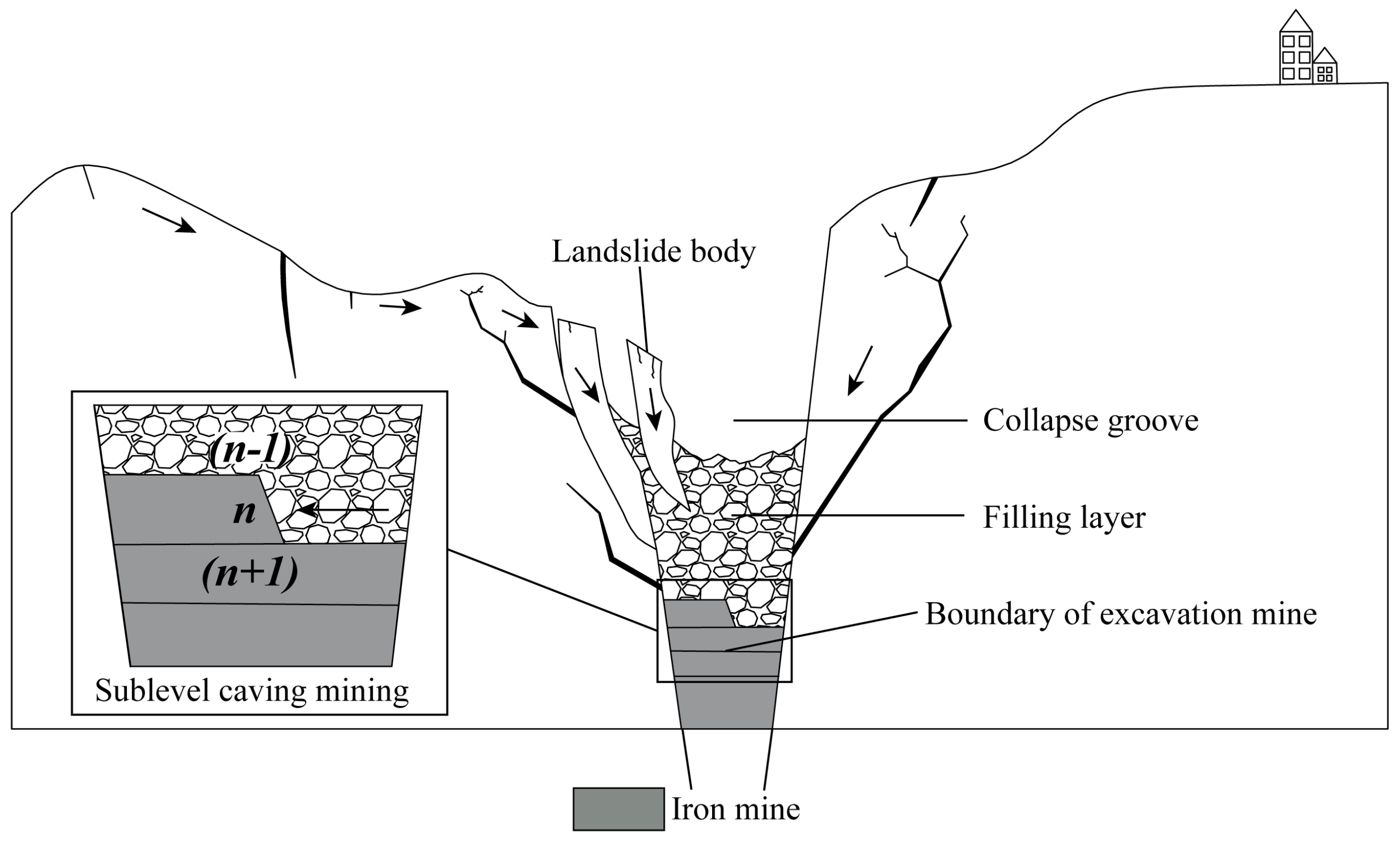
2. Progressive Slope Failure Induced by Sublevel Caving Mining
3. Methodology
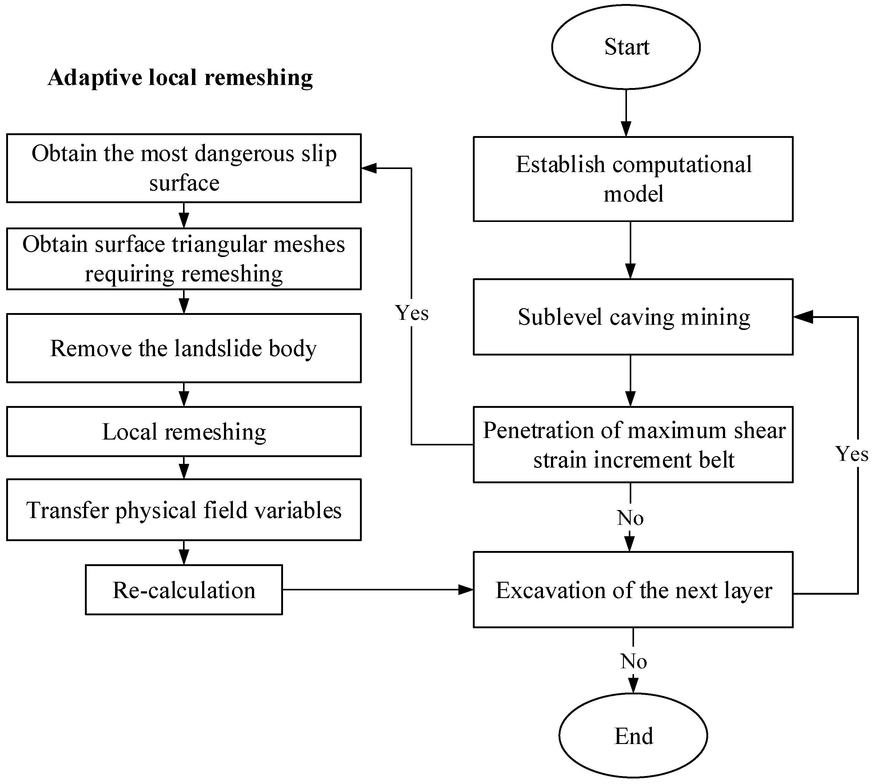
3.1. Overview
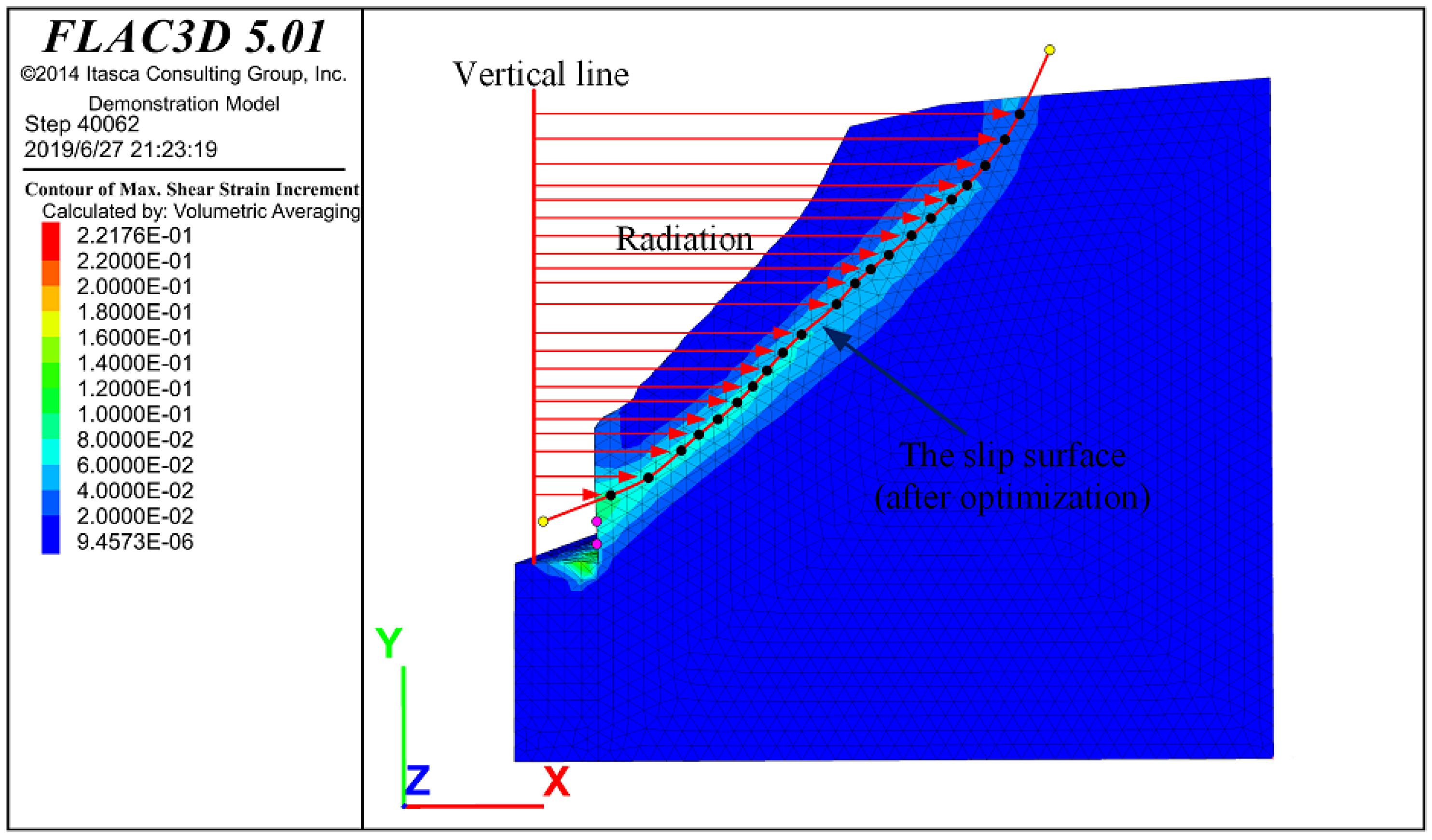
3.2. Acquisition of the Most Dangerous Slip Surface
3.2.1. Searching for the Slip Surface
3.2.2. Acquisition of the Slip Surface
- (1)
- A vertical line is set at the position of the ore vein from the top position of the filling layer.
- (2)
- Radiation is incrementally emitted from the vertical line toward the direction of the rock mass from the bottom of the vertical line.
- (3)
- The mesh with the highest shear strain is obtained by comparing the magnitude of the shear strain increment of the meshes on the horizontal rays, and the centroid of the mesh with the highest shear strain is taken as the maximum shear strain increment point.
- (4)
- The maximum shear strain increment points for all rays are determined. The results are indicated by the black and pink points in Figure 4.
- (5)
- (6)
- The least-squares method is used to adjust these points, and the optimized points are connected to form a smooth curve (Figure 4).
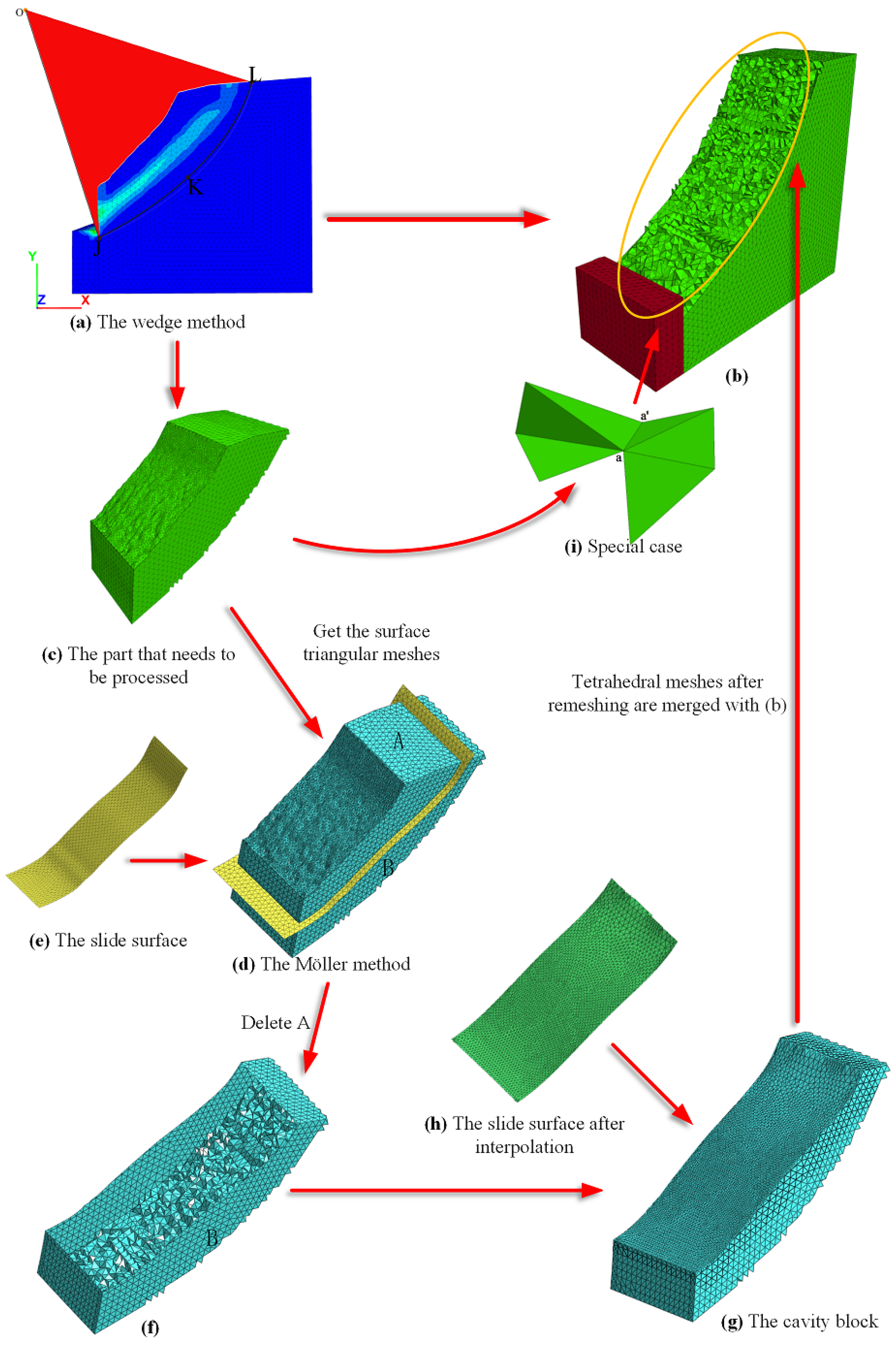
3.3. Acquisition and Adjustment of the Surface Triangular Mesh
- (1)
- The abovementioned mesh with excessive deformation is divided into two parts using the most dangerous slip surface.
- (2)
- Part 1: This part is the landslide body between the slip surface and free surface. We can simulate a landslide by removing the landslide body.
- (3)
- Part 2: This part of the mesh is located near the slip surface. A part of the mesh is stretched because of the landslide, and the deformation of the mesh is either considerable or the mesh is completely deformed. Therefore, this part of the mesh requires remeshing.
- (1)
- Determine the points J, K, and L at the outer edge of the maximum shear increment belt.
- (2)
- Form a sector with O as the center.
- (3)
- Form the wedge space. The distortion zone is divided into a landslide body portion and a remeshing portion through the most dangerous slip surface.
3.3.1. Acquisition of the Surface Triangular Mesh
- (1)
- Features of the tetrahedral mesh
- (2)
- Special case
3.3.2. Adjustment of the Surface Triangular Mesh
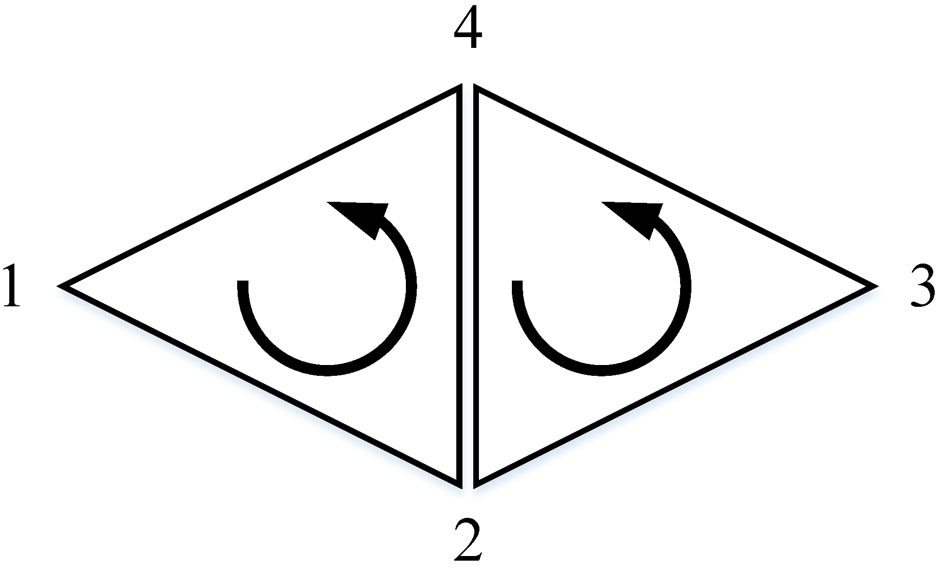
- Step 1:
- The order of the three nodes of a triangle is adjusted to be counterclockwise, and the triangle is marked as T1, indicating that the order of the nodes of the triangle has been adjusted.
- Step 2:
- The neighboring triangles of T1 that have shared edges are searched. If the order of the shared edge nodes of the neighboring triangle is counterclockwise, the order of the nodes of the triangle is adjusted and the triangle is marked as T2.
- Step 3:
- The neighboring triangles of T2 that have shared edges are searched. If the order of the shared edge nodes of the neighboring triangle is counterclockwise, the order of the nodes of the triangle is adjusted and the triangle is marked.
- Step 4:
- This cycle is repeated until all the triangles are marked.
3.4. Local Remeshing of the Distorted Mesh
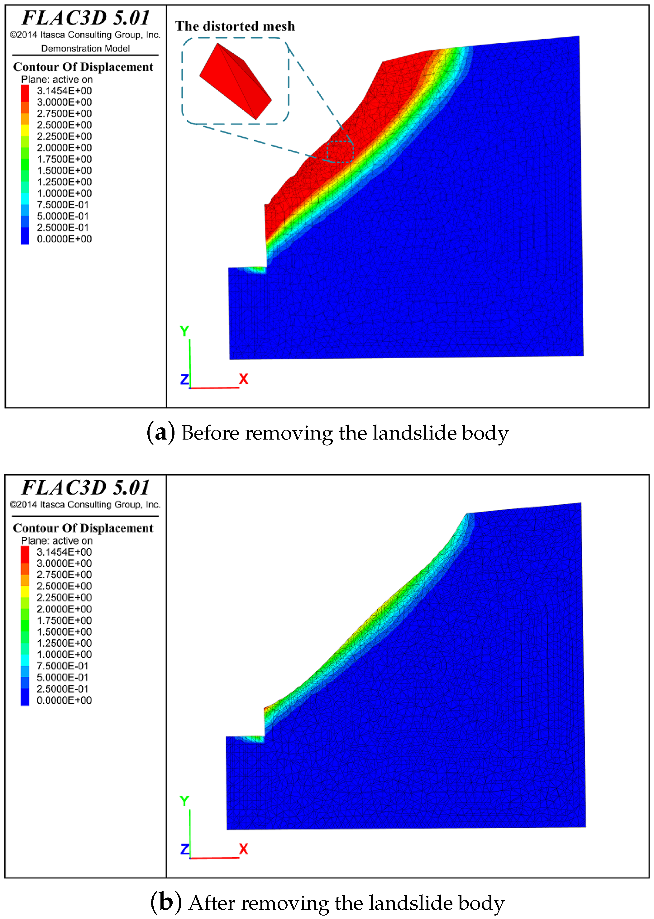
3.4.1. Removal of the Landslide Body
3.4.2. Tetrahedral Mesh Remeshing
3.5. Transfer of the Physical Field Variables
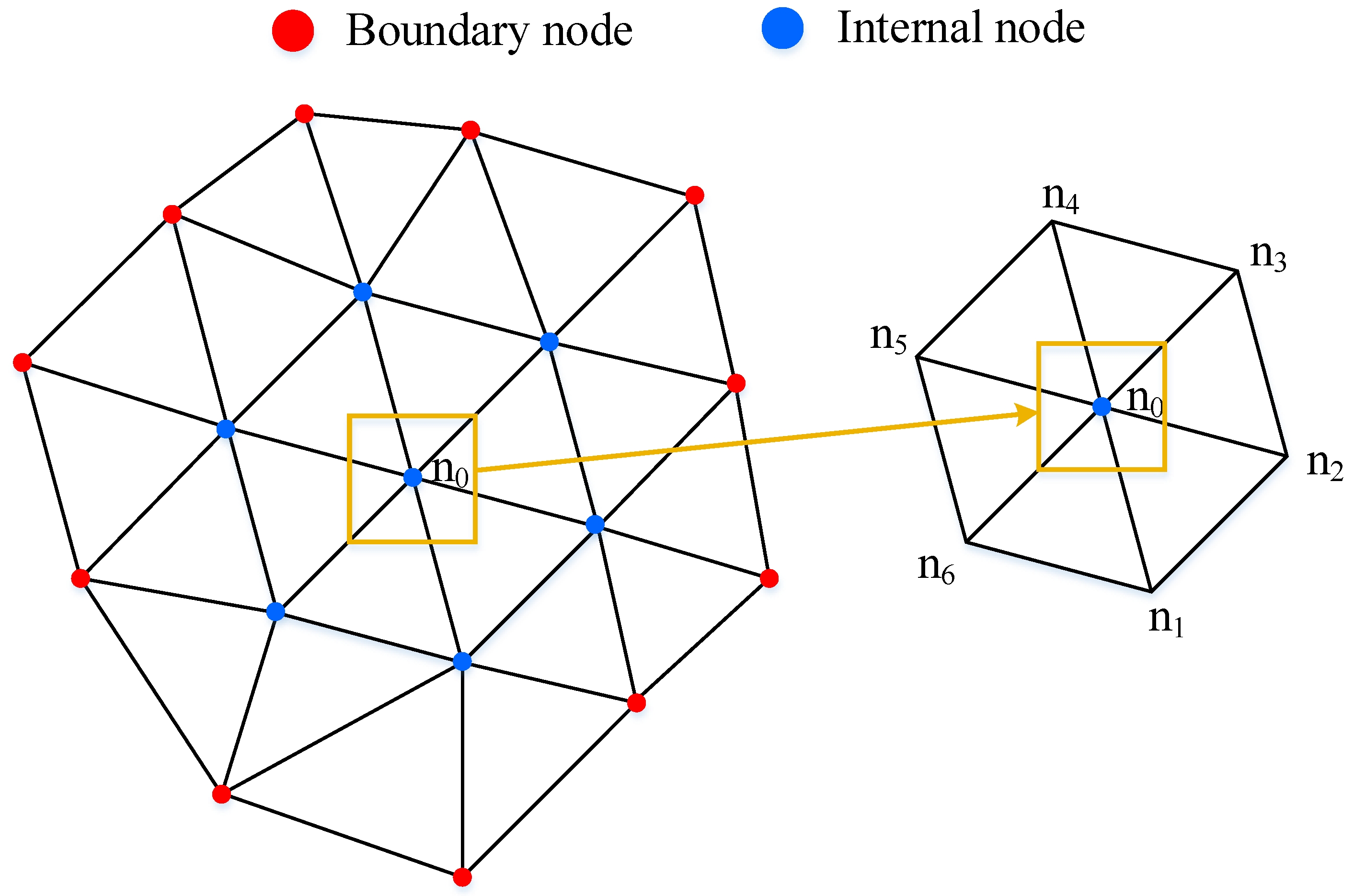
- (1)
- Transfer the stress of the old meshes to the old nodes to obtain the equivalent mesh physical field variables of the old nodes.
- (2)
- Determine the relationship between the new node and the old mesh. This step requires the new mesh node to be inside the old mesh.
- (3)
- Transfer the equivalent mesh stresses of the old nodes to the new nodes. The equivalent mesh stresses of the nodes and the shape function can be used to interpolate the value of the stresses at any position in the mesh; see Equations (1) and (2).where [N] is the shape function of the original mesh, and ui, uj, uk, and ul are the physical field variables of the original mesh.where [] is the shape function of the new node; are the coordinates of the new node; and (, , ) are the coordinates of the original node, .
- (4)
- Acquire the physical field variables of the new meshes; see Equation (3).where is the equivalent physical field variables of node j of mesh i; is the physical field variables of mesh i.
4. Verification
5. Application Case
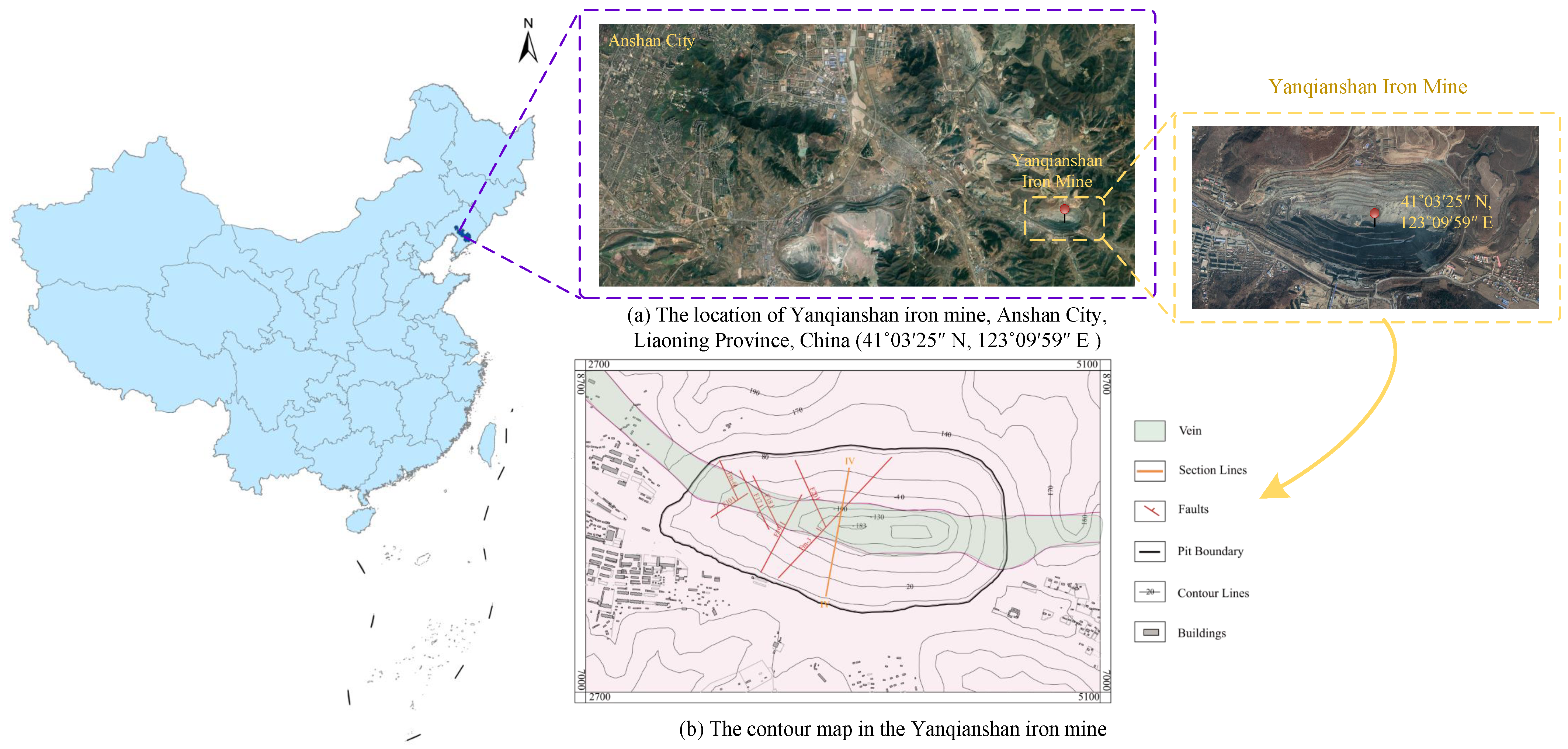
5.1. Geological and Engineering Background
5.1.1. Geology
5.1.2. Engineering Background
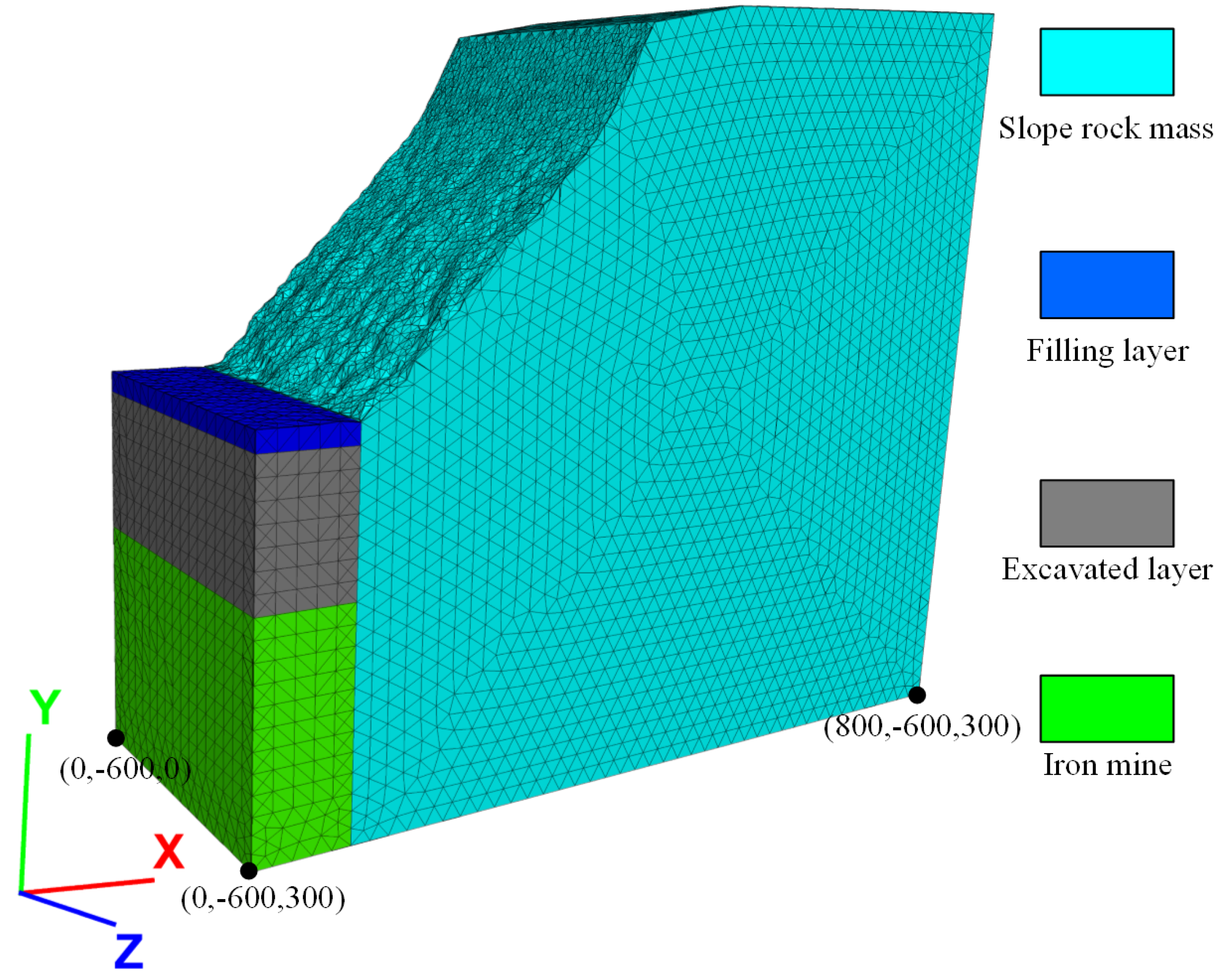
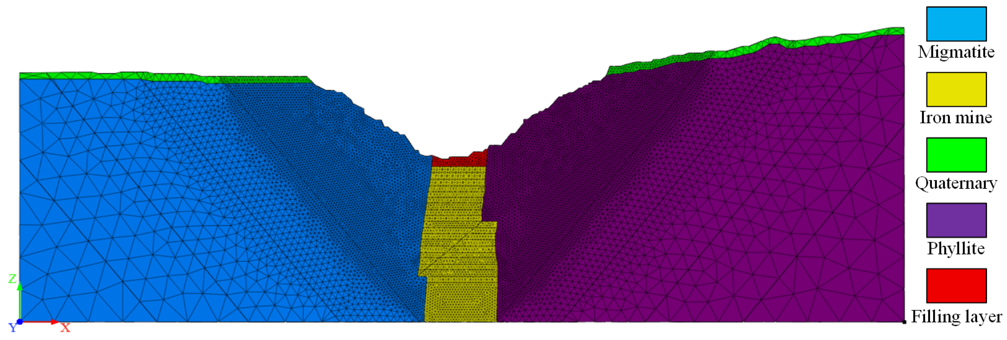
5.2. Computational Model and Parameters
5.2.1. Computational Model
5.2.2. Computational Parameters
5.3. Process of Numerical Modeling
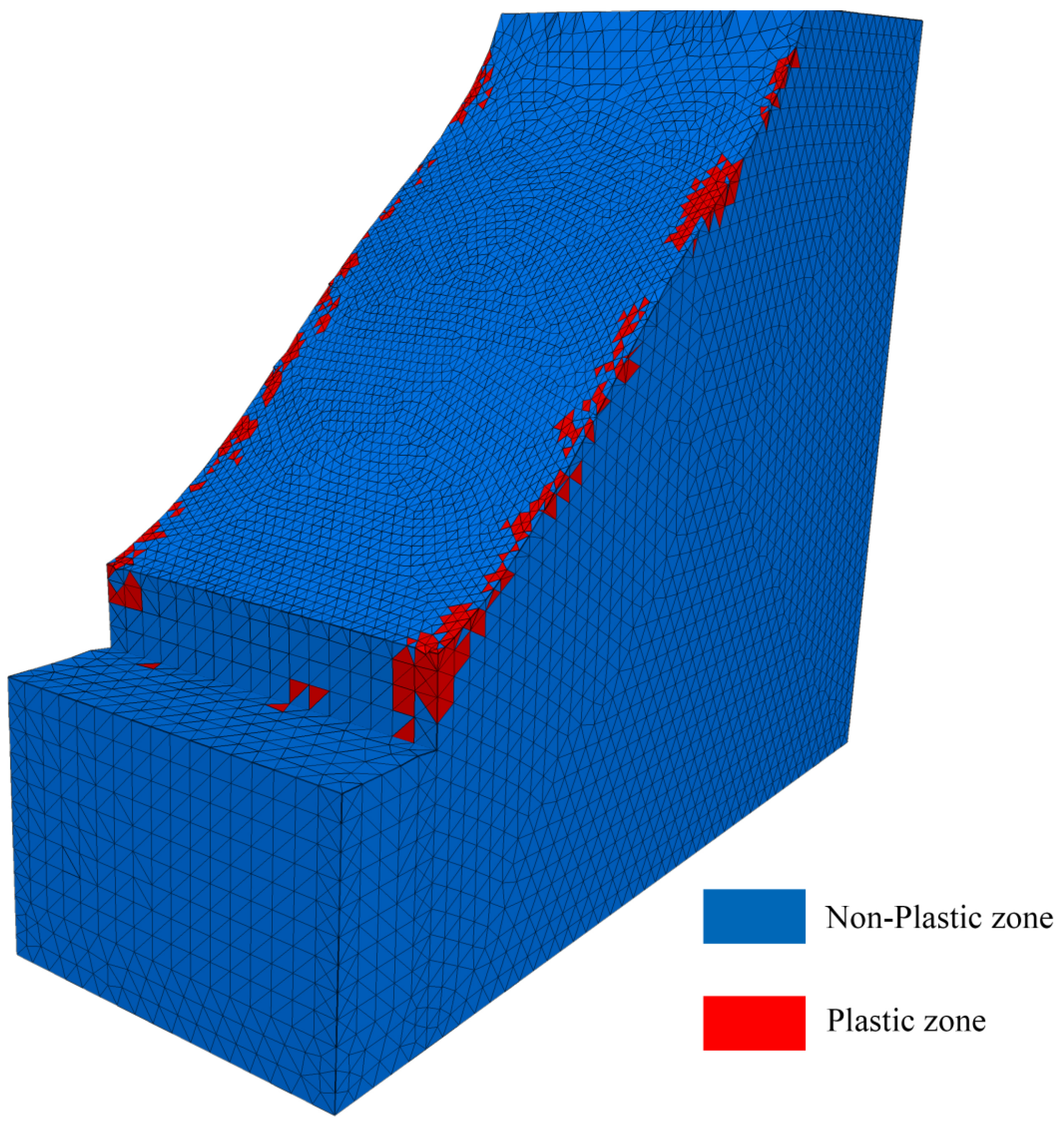
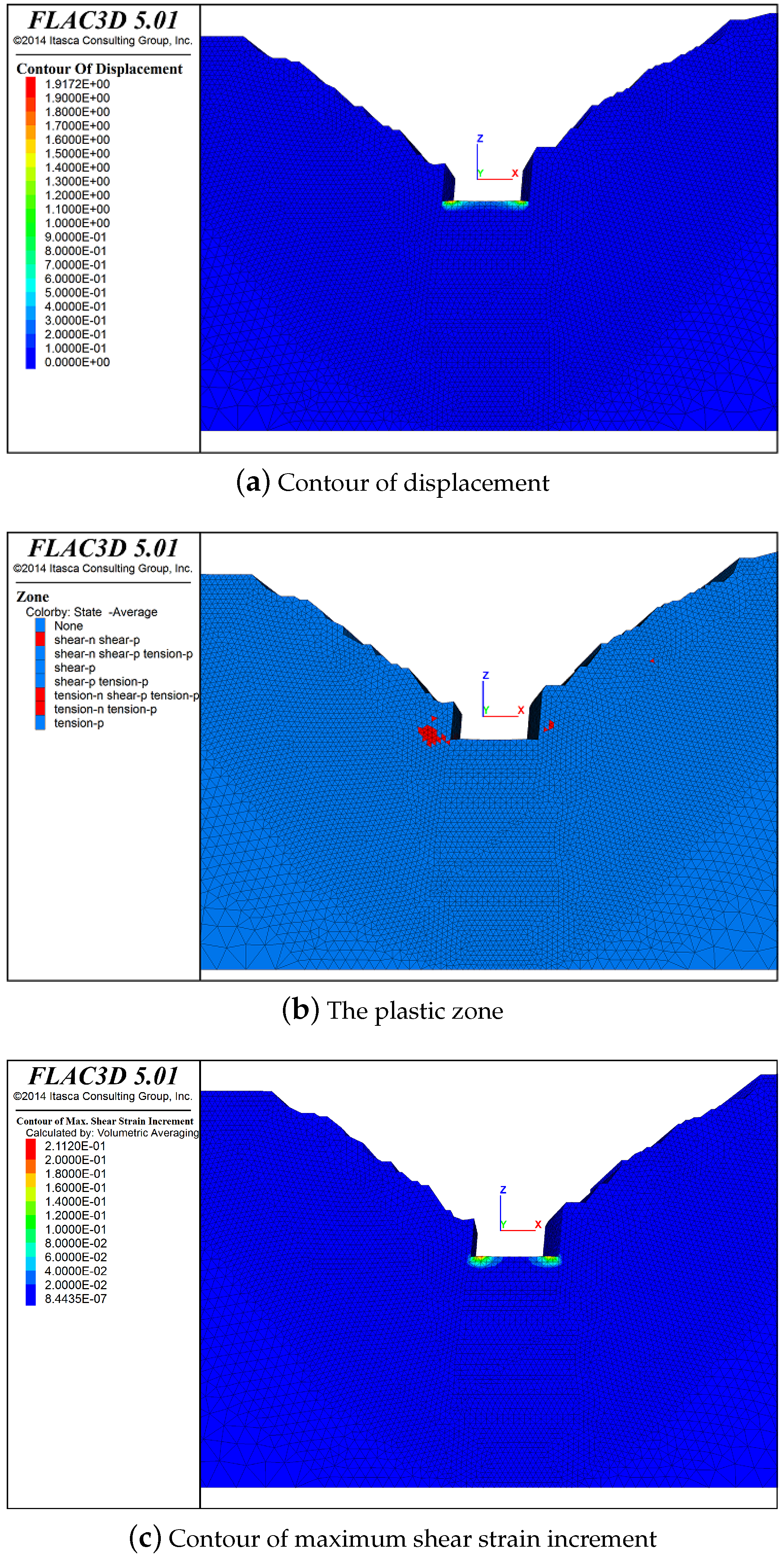
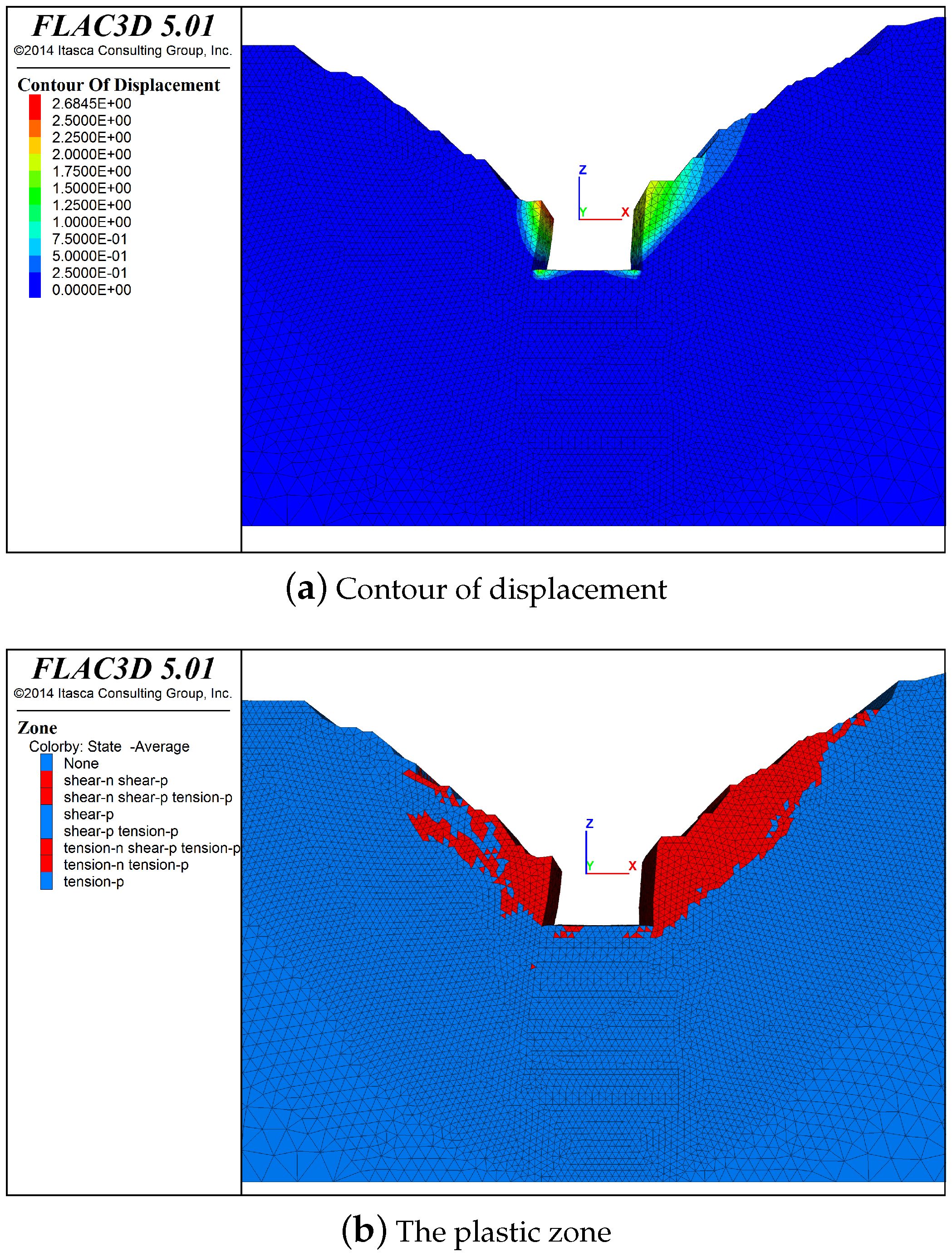
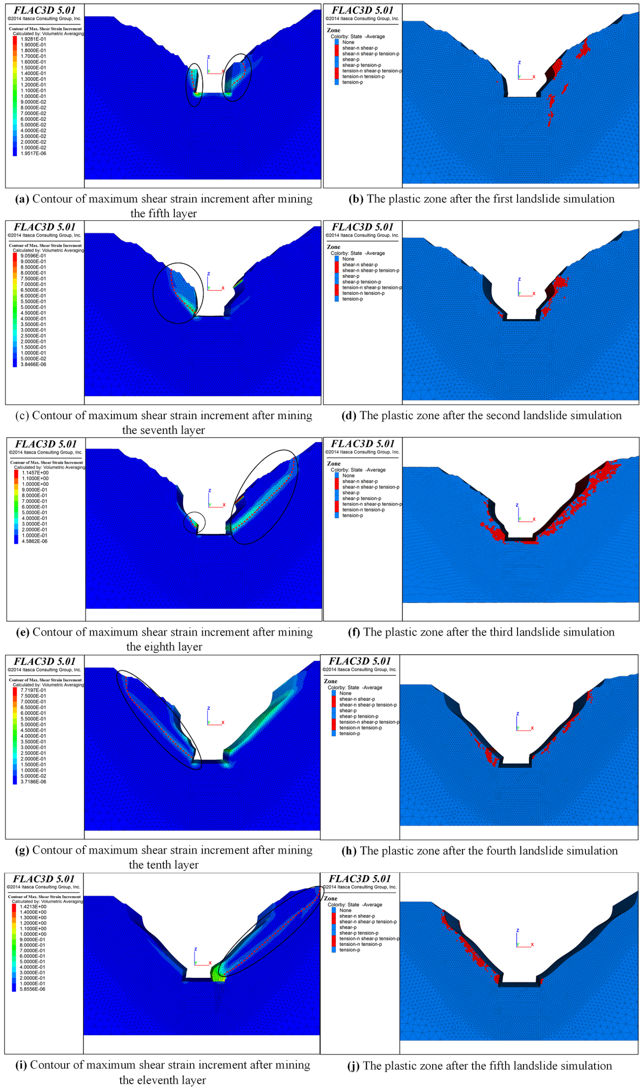
5.3.1. Modeling of the Excavation of the First to Fourth Layers
5.3.2. Modeling of the Excavation of the Fifth and Sixth Layers
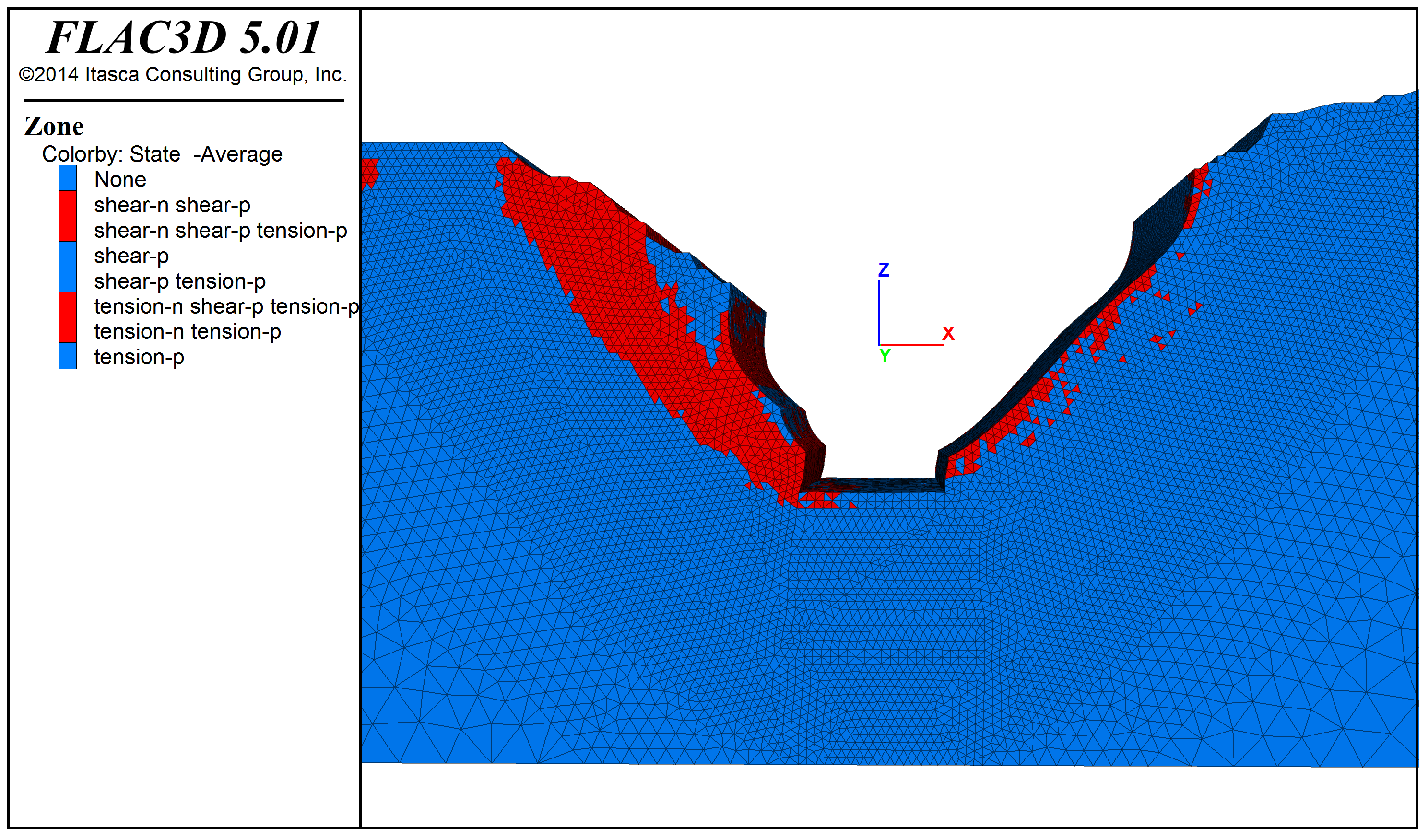
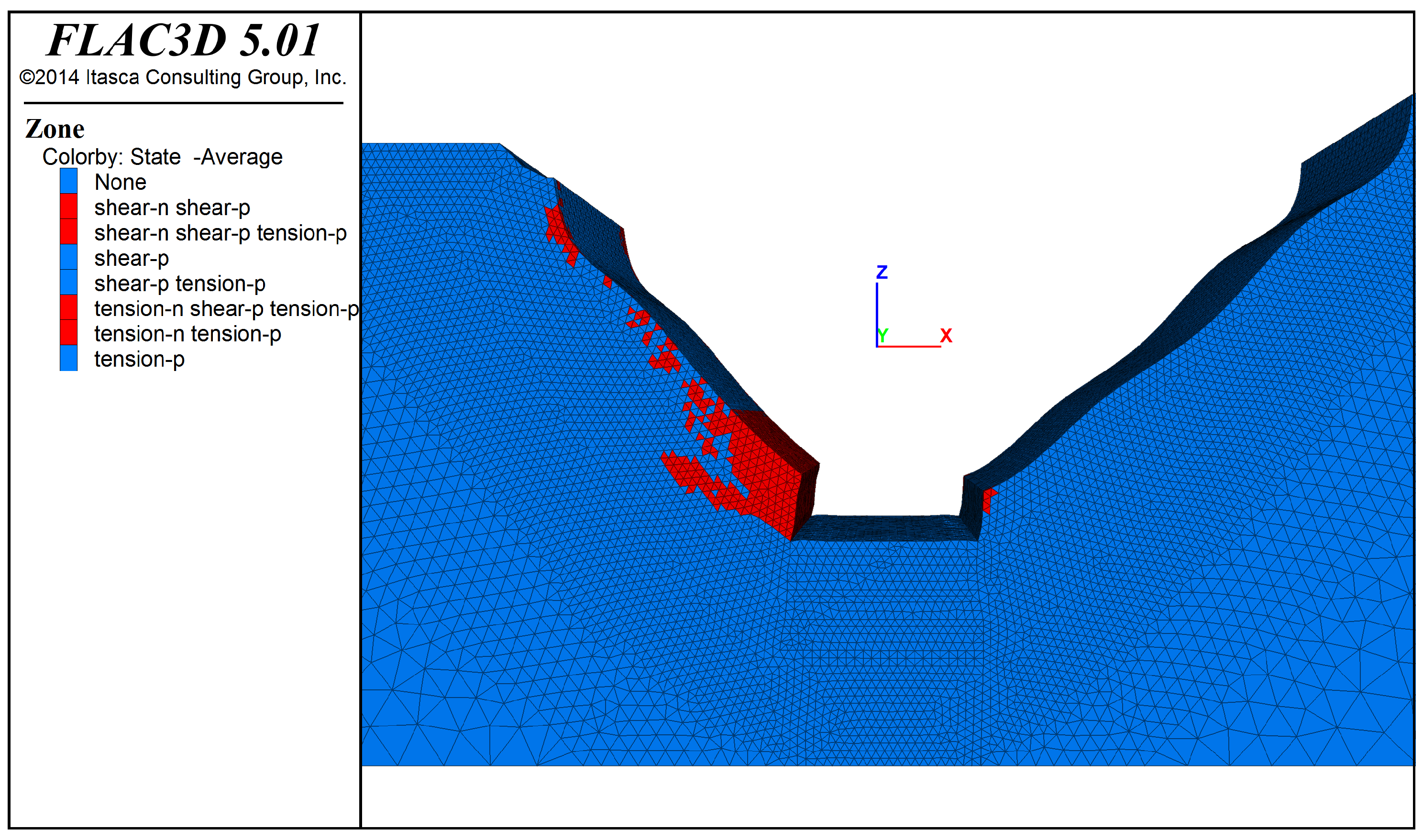
5.3.3. Modeling of the Excavation of the Seventh to Twelfth Layers
6. Discussion
6.1. Advantages of the Proposed Method for Analyzing Progressive Slope Failure
6.2. Disadvantages of the Proposed Method for Analyzing Progressive Slope Failure
6.3. Outlook and Future Work
7. Conclusions
Author Contributions
Funding
Institutional Review Board Statement
Informed Consent Statement
Data Availability Statement
Acknowledgments
Conflicts of Interest
Abbreviations
| LREM | Finite Difference Modeling Method using Adaptive Local Remeshing |
| FLAC | Fast Lagrangian Analysis of Continua |
| DEM | Discrete Element Method |
| FDM | Finite Difference Method |
| FEM | Finite Element Method |
| FOS | Factor of Safety |
| SRM | Strength Reduction Method |
| MPM | Material Point Method |
References
- Huang, C.; Lo, C.; Jang, J.; Hwu, L. Internal soil moisture response to rainfall-induced slope failures and debris discharge. Eng. Geol. 2008, 101, 134–145. [Google Scholar] [CrossRef]
- Mohammadi, S.; Taiebat, H. Finite element simulation of an excavation-triggered landslide using large deformation theory. Eng. Geol. 2016, 205, 62–72. [Google Scholar] [CrossRef]
- Govender, N.; Wilke, D.N.; Kok, S.; Els, R. Development of a convex polyhedral discrete element simulation framework for NVIDIA Kepler based GPUs. J. Comput. Appl. Math. 2014, 270, 386–400. [Google Scholar] [CrossRef]
- Govender, N.; Wilke, D.N.; Kok, S. Collision detection of convex polyhedra on the NVIDIA GPU architecture for the discrete element method. Appl. Math. Comput. 2015, 267, 810–829. [Google Scholar] [CrossRef]
- Souley, M.; Homand, F. Stability of jointed rock masses evaluated by UDEC with an extended Saeb-Amadei constitutive law. Int. J. Rock Mech. Min. Sci. Geomech. Abstr. 1996, 33, 233–244. [Google Scholar] [CrossRef]
- Li, X.; Wu, Y.; He, S.; Su, L.J. Application of the material point method to simulate the post-failure runout processes of the Wangjiayan landslide. Eng. Geol. 2016, 212. [Google Scholar] [CrossRef]
- Wang, B.; Vardon, P.; Hicks, M. Rainfall-induced slope collapse with coupled material point method. Eng. Geol. 2018, 239. [Google Scholar] [CrossRef]
- Conte, E.; Pugliese, L.; Troncone, A. Post-failure stage simulation of a landslide using the material point method. Eng. Geol. 2019, 253, 149–159. [Google Scholar] [CrossRef]
- Bakhtavar, E. Transition from Open-Pit to Underground in the Case of Chah-Gaz Iron Ore Combined Mining. J. Min. Sci. 2013, 49, 955–966. [Google Scholar] [CrossRef]
- Elmo, D.; Vyazmensky, A.; Stead, D.; Rance, J.R. A Hybrid FEM/DEM Approach to Model the Interaction between Open-Pit and Underground Block-Caving Mining; Rock Mechanics: Meeting Society’s Challenges and Demands, Vols 1 and 2: Vol: Fundamentals, New Technologies & New Ideas; Vol 2: Case Histories; CRC Press: Boca Raton, FL, USA, 2007; pp. 1287–1294. [Google Scholar] [CrossRef]
- Vyazmensky, A.; Stead, D.; Elmo, D.; Moss, A. Numerical Analysis of Block Caving-Induced Instability in Large Open Pit Slopes: A Finite Element/Discrete Element Approach. Rock Mech. Rock Eng. 2010, 43, 21–39. [Google Scholar] [CrossRef]
- Sun, C.; Chai, J.; Xu, Z.; Qin, Y.; Chen, X. Stability charts for rock mass slopes based on the Hoek-Brown strength reduction technique. Eng. Geol. 2016, 214, 94–106. [Google Scholar] [CrossRef]
- Zienkiewicz, O.; Humpheson, C.; Lewis, R. Associated and nonassociated visco-plasticity and plasticity in soil mechanics. Geotechnique 1975, 25, 671–689. [Google Scholar] [CrossRef]
- Kumsar, H.; Aydan, O.; Ulusay, R. Dynamic and static stability assessment of rock slopes against wedge failures. Rock Mech. Rock Eng. 2000, 33, 31–51. [Google Scholar] [CrossRef]
- Zhao, Y.; Yang, T.; Bohnhoff, M.; Zhang, P.; Yu, Q.; Zhou, J.; Liu, F. Study of the Rock Mass Failure Process and Mechanisms During the Transformation from Open-Pit to Underground Mining Based on Microseismic Monitoring. Rock Mech. Rock Eng. 2018, 51, 1473–1493. [Google Scholar] [CrossRef]
- Woo, K.S.; Eberhardt, E.; As, A. Characterization and empirical analysis of block caving induced surface subsidence and macro deformations. In Proceedings of the 3rd Canada-US Rock Mechanics Symposium and 20th Canadian Rock Mechanics Symposium, Toronto, ON, Canada, 9–15 May 2009; pp. 1–10. [Google Scholar]
- Janelid, I.; Kvapil, R. Sublevel caving. Int. J. Rock Mech. Min. Sci. 1966, 3, 129–153. [Google Scholar] [CrossRef]
- Zhou, X.P.; Cheng, H. Stability analysis of three-dimensional seismic landslides using the rigorous limit equilibrium method. Eng. Geol. 2014, 174, 87–102. [Google Scholar] [CrossRef]
- Liu, Z.; Liu, J.; Bian, K.; Ai, F. Three-dimensional limit equilibrium method based on a TIN sliding surface. Eng. Geol. 2019, 262, 105325. [Google Scholar] [CrossRef]
- Saiang, D. Stability analysis of the blast-induced damage zone by continuum and coupled continuum-discontinuum methods. Eng. Geol. 2010, 116, 1–11. [Google Scholar] [CrossRef]
- Zheng, W.; Zhuang, X.; Tannant, D.D.; Cai, Y.; Nunoo, S. Unified continuum/discontinuum modeling framework for slope stability assessment. Eng. Geol. 2014, 179, 90–101. [Google Scholar] [CrossRef]
- Tomas, R.; Cuenca, A.; Cano, M.; Garcia-Barba, J. A graphical approach for slope mass rating (SMR). Eng. Geol. 2012, 124, 67–76. [Google Scholar] [CrossRef]
- Basahel, H.; Mitri, H. Application of rock mass classification systems to rock slope stability assessment: A case study. J. Rock Mech. Geotech. Eng. 2017, 9, 5–21. [Google Scholar] [CrossRef]
- Mohammad, A.; Yaser, A.N.; Lila, R.; Haluk, A.; Jafar, R.; Reza, D.; Amir, R. Application of the modified Q-slope classification system for sedimentary rock slope stability assessment in Iran. Eng. Geol. 2019, 264, 105349. [Google Scholar] [CrossRef]
- Möller, T. A Fast Triangle-triangle Intersection Test. J. Graph. Tools 1997, 2, 25–30. [Google Scholar] [CrossRef]
- Tropp, O.; Tal, A.; Shimshoni, I. A fast triangle to triangle intersection test for collision detection. Comput. Animat. Virtual Worlds 2006, 17, 527–535. [Google Scholar] [CrossRef]
- Shen, H.; Heng, P.; Tang, Z. A Fast Triangle-triangle Overlap Test Using Signed Distances. J. Graph. Tools 2003, 8, 17–23. [Google Scholar] [CrossRef]
- Guigue, P.; Devillers, O. Fast and Robust Triangle-Triangle Overlap Test Using Orientation Predicates. J. Graph. Tools 2003, 8, 25–32. [Google Scholar] [CrossRef]
- Mei, G.; Tipper, J.C.; Xu, N. A Generic Paradigm for Accelerating Laplacian-Based Mesh Smoothing on the GPU. Arab. J. Sci. Eng. 2014, 39, 7907–7921. [Google Scholar] [CrossRef]
- Xu, N.; Zhang, J.; Tian, H.; Mei, G.; Ge, Q. Discrete element modeling of strata and surface movement induced by mining under open-pit final slope. Int. J. Rock Mech. Min. Sci. 2016, 88, 61–76. [Google Scholar] [CrossRef]
- Liu, G.R.; Zhang, G.Y. Edge-based smoothed point interpolation methods. Int. J. Comput. Methods 2011, 5, 621–646. [Google Scholar] [CrossRef]


| Name | C (MPa) | () | E (GPa) | (kg/m3) | |
|---|---|---|---|---|---|
| Iron Mine | 0.95 | 41 | 40 | 0.2 | 3100 |
| Slope Rock Mass | 0.45 | 39 | 18 | 0.23 | 2670 |
| Filling Layer | 0 | 25 | 6 | 0.32 | 1550 |
| Slicing Mining (After Exploiting the ith Layer) | 1st Layer | 2nd Layer | 3rd Layer | 4th Layer | 5th Layer | 6th Layer | 7th Layer | 8th Layer | After the 1st Landslide |
|---|---|---|---|---|---|---|---|---|---|
| Slope Stability (LREM) | Stable | Stable | Stable | Stable | Stable | Stable | Stable | Unstable | Stable |
| Safety Factors (FDM+SRM) | 1.49 | 1.43 | 1.35 | 1.27 | 1.19 | 1.12 | 1.05 | 1 | 1.39 |
| Slicing Mining | 1st Layer | 2nd Layer | 3rd Layer | 4st Layer | 5st Layer | 6st Layer | 7st Layer | 8st Layer | 9st Layer | 10th Layer | 11th Layer | 12th Layer |
|---|---|---|---|---|---|---|---|---|---|---|---|---|
| Thickness (m) | 17.5 | 19.7 | 18.9 | 17.0 | 16.5 | 15.2 | 20.8 | 15.5 | 17.9 | 18.6 | 16.6 | 16.9 |
| Width (m) | 158.1 | 158.2 | 159.7 | 163.1 | 163.9 | 163.7 | 163.3 | 164.3 | 167.2 | 212.9 | 213.8 | 213.7 |
| Length (m) | 300 | 300 | 300 | 300 | 300 | 300 | 300 | 300 | 300 | 300 | 300 | 300 |
| Name | C (MPa) | () | E (GPa) | (kg/m3) | |
|---|---|---|---|---|---|
| Iron Mine | 0.95 | 41 | 40 | 0.2 | 3100 |
| Migmatite | 0.45 | 39 | 18 | 0.23 | 2670 |
| Phyllite | 0.365 | 36.5 | 15 | 0.25 | 2740 |
| Quaternary | 0.2 | 25 | 0.05 | 0.3 | 1980 |
| Filling Layer | 0 | 24 | 0.06 | 0.32 | 1550 |
Publisher’s Note: MDPI stays neutral with regard to jurisdictional claims in published maps and institutional affiliations. |
© 2021 by the authors. Licensee MDPI, Basel, Switzerland. This article is an open access article distributed under the terms and conditions of the Creative Commons Attribution (CC BY) license (https://creativecommons.org/licenses/by/4.0/).
Share and Cite
Tu, J.; Zhang, Y.; Mei, G.; Xu, N. Numerical Investigation of Progressive Slope Failure Induced by Sublevel Caving Mining Using the Finite Difference Method and Adaptive Local Remeshing. Appl. Sci. 2021, 11, 3812. https://doi.org/10.3390/app11093812
Tu J, Zhang Y, Mei G, Xu N. Numerical Investigation of Progressive Slope Failure Induced by Sublevel Caving Mining Using the Finite Difference Method and Adaptive Local Remeshing. Applied Sciences. 2021; 11(9):3812. https://doi.org/10.3390/app11093812
Chicago/Turabian StyleTu, Jingzhi, Yanlin Zhang, Gang Mei, and Nengxiong Xu. 2021. "Numerical Investigation of Progressive Slope Failure Induced by Sublevel Caving Mining Using the Finite Difference Method and Adaptive Local Remeshing" Applied Sciences 11, no. 9: 3812. https://doi.org/10.3390/app11093812
APA StyleTu, J., Zhang, Y., Mei, G., & Xu, N. (2021). Numerical Investigation of Progressive Slope Failure Induced by Sublevel Caving Mining Using the Finite Difference Method and Adaptive Local Remeshing. Applied Sciences, 11(9), 3812. https://doi.org/10.3390/app11093812