Instrumental Uncertainty of Conductance Transducers for Maritime Reduced-Scale Models

Abstract

This paper aims to determine the instrumental measurement uncertainty of conductance transducers for maritime reduced-scale models developed in hydraulic experimental facilities. These transducers are used for the measurements of wave levels and their variations under a dynamic regime (being the measurement principle and method briefly described in the paper). Several metrological characterization methods are also presented, aiming to identify and quantify measurement uncertainty components, namely electrical stability, linearity, reversibility, repeatability, and thermal influence. The obtained results were applied in the evaluation of the transducer instrumental measurement uncertainty.

1. Introduction

For several decades, conductance transducers have been developed and applied by LNEC to maritime reduced-scale models, in order to obtain the measurement of a wave level and its variation under a dynamic regime, namely using infrastructures able to generate waves in hydraulic experimental facilities. Coastal engineering is a branch of civil engineering with a large impact in economic development, contributing for many types of studies, namely wave mechanics, shoreline erosion, and methods to protect the shore from extreme events (e.g., climatic, geological), and harbor design, among others.

Studies often combine field observation with laboratory modeling observation and mathematical and computational calculus [1]. Laboratory studies are usually related with physical models, aiming to reproduce, at a certain scale, a physical system often providing information to the development of numerical models for hydrodynamic phenomena, leading to a modern perspective of “Hybrid Modeling” that combines the contributions of physical models through boundary conditions with complex interaction models of fluid flow regimes. This approach was recently named “Composite Modeling”, being a methodology that balances the use of physical and numerical models [2]. The use of physical modeling is applied in many different domains of hydraulic engineering [3], making use of many types of models and planning approaches, in order to obtain advantages that physical models still provide [3].

Coastal and nearshore hydrodynamics are included in this context where measurement in physical models are used to analyze the travel of waves from deep waters to shallower regions, and the related effects of energy transfer and turbulence, creating complex non-linear interactions [4]. For these types of studies, laboratory experiments play a relevant role in research and development [5].

The experimental approach with physical models has been used with relevant results to provide information for decision-making processes regarding problems of coastal erosion by studying the impact of coastal structures (e.g., breakwaters, seawalls, dikes, and revetments) intended to reduce wave energy, sediment transport, and other effects of hydrodynamic nature [6]. The same applies to the development of harbors and maritime structures, regarding the analysis of complex processes of wave propagation and its interaction with coastal structures. In a laboratory, the development of experimental testing using wave generation in order to evaluate its behavior in time and frequency domains requires the use of measurement instruments that re able to obtain accurate observations within a time response suitable for the phenomena requirements.

The metrological characterization and traceability of measurement instruments play a critical role in the laboratory-based research, providing the quality of measurement that is useful in the analysis of hydraulic processes, but also robust raw data for numerical model parameterization and for its validation [7,8].

This study proposes several metrological characterization methods applied to conductance transducers, integrated in SI traceability chains, and allows the determination of measurement uncertainty components, which contribute for the wave level instrumental measurement uncertainty. Due to the nature of the conductance transducer measurement principle and method, metrological characteristics, such as electrical stability, linearity, reversibility, repeatability, and thermal influence, should be known and used to evaluate if the applied transducer complies with instrumental requirements defined for the experimental observation scenario, in addition to quality production control procedures. A more robust instrumental comparison with other available measurement transducers can also be performed, contributing for the improvement of the experimental design. This knowledge, which reflects a part of the overall level measurement accuracy, can also be used to identify the main instrumental uncertainty contributions, which can be targeted for upgrading from a design and production point of view. The conductance transducer instrumental uncertainty can also be introduced in hydraulic computational activities, therefore, improving the physical representative of the performed simulations.

Section 2 of this paper provides a brief description of the measurement principle and method related to LNEC’s conductance transducers, which are applied in maritime reduced-scale models. In Section 3, the proposed metrological characterization methods are described, being the obtained experimental results shown in Section 4. Section 5 is dedicated to the evaluation of the instrumental measurement accuracy, including the probabilistic formulation of the identified uncertainty components, and its propagation to the wave level, by the GUM method. At last, the discussion of obtained results is presented in Section 6.

2. LNEC Conductance Transducer for Maritime Reduced-Scale Models

The measurement principle related to the LNEC conductance transducer is supported in the electrical resistance established between two metallic electrodes vertically immersed in water. This electrical quantity is influenced by the water resistivity, ρ, the distance between the two electrodes, D, the electrodes diameters, d₁ and d₂, and the water level, h, being expressed by

$$R=\frac{\rho }{2\pi }·\frac{1}{h}·\ln \left(\frac{4D^2}{d_1·d_2}\right),$$

(1)

when d₁ and d₂ are equal or lower than 0.25 D.

If the water resistivity can be assumed constant or compensated, the inverse resistance between the two vertical electrodes, which corresponds to the conductance quantity, G (expressed in Siemens), is directly proportional to the water level, thus allowing to measure this quantity in maritime hydraulic experimental activities. Conductance transducers are connected to a power supply and a signal conditioner, which provides an output voltage, usually recorded by a data acquisition system.

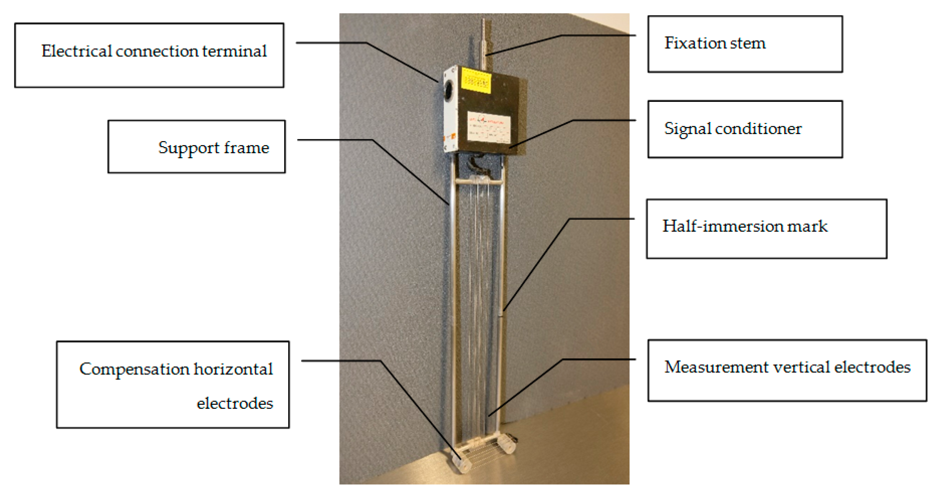
The conductance transducers developed by LNEC (an example is shown in Figure 1), have an input voltage of 15 V (DC) and their output voltage varies between 0 V and 10 V (DC), available in different sizes and, therefore, covering a wide range of wave level measurement in experimental activities involving maritime reduced-scale models.

In order to reduce the measurement uncertainty related to the variation of the water resistivity during and between experimental sets of measurements, additional compensation horizontal electrodes were considered in the lower region of the sensor (see Figure 1).

The main concerns regarding to this type of conductance transducer are corrosion, water electrolysis and polarization effects in the metallic electrodes.

3. Metrological Characterization Methods

3.1. Electrical Stability

This section describes the proposed characterization method of the conductance transducer’s electrical stability. The nature of this type of transducer, where a relation between the dimensional quantity (the water level) and the electrical quantity (output voltage) is defined, justifying the characterization of the transducer’s electrical behavior, namely, of its stability. The proposed electrical testing can be performed, in a first stage, for production quality control and maintenance purposes and, in a second stage, as a preliminary test performed in laboratory or in field, characterized by different electrical environments.

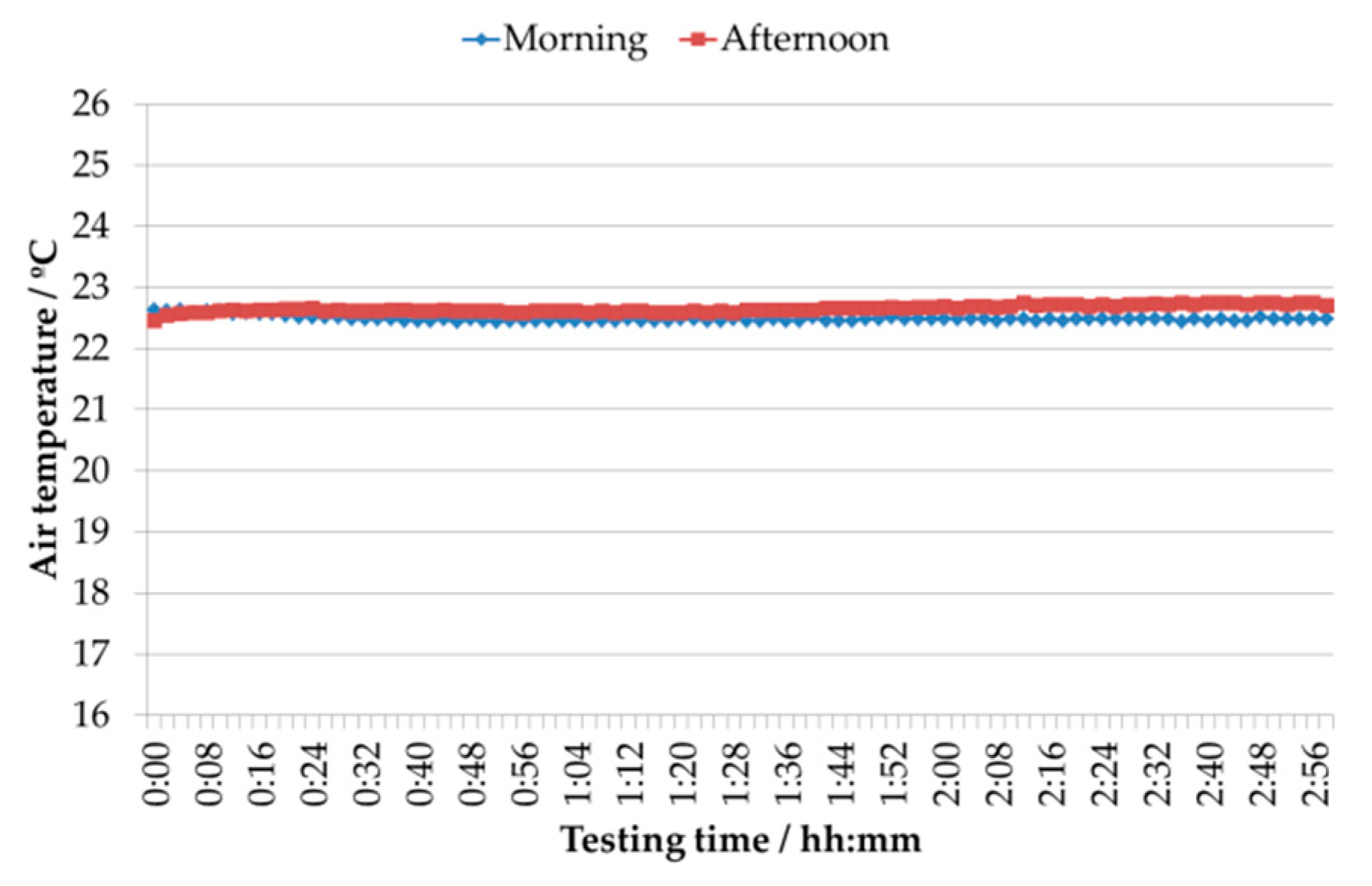
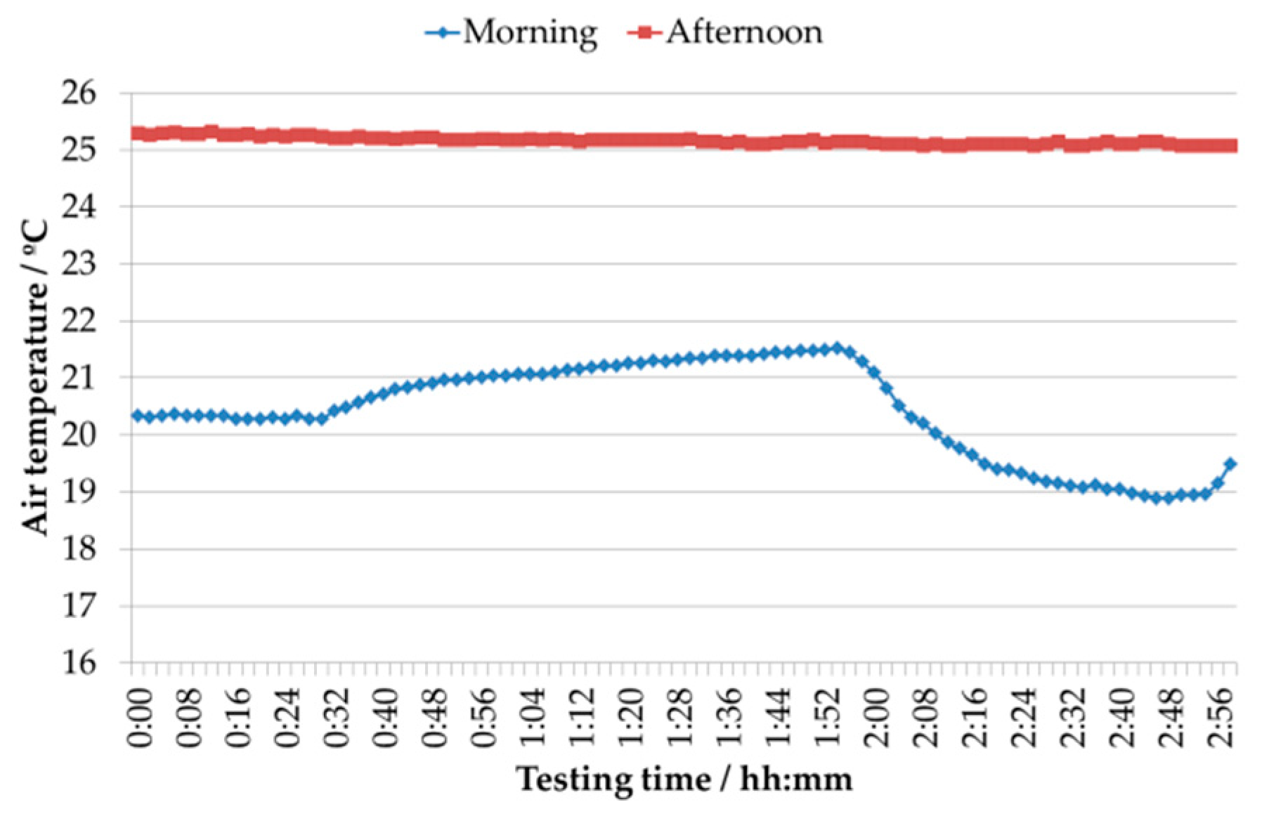
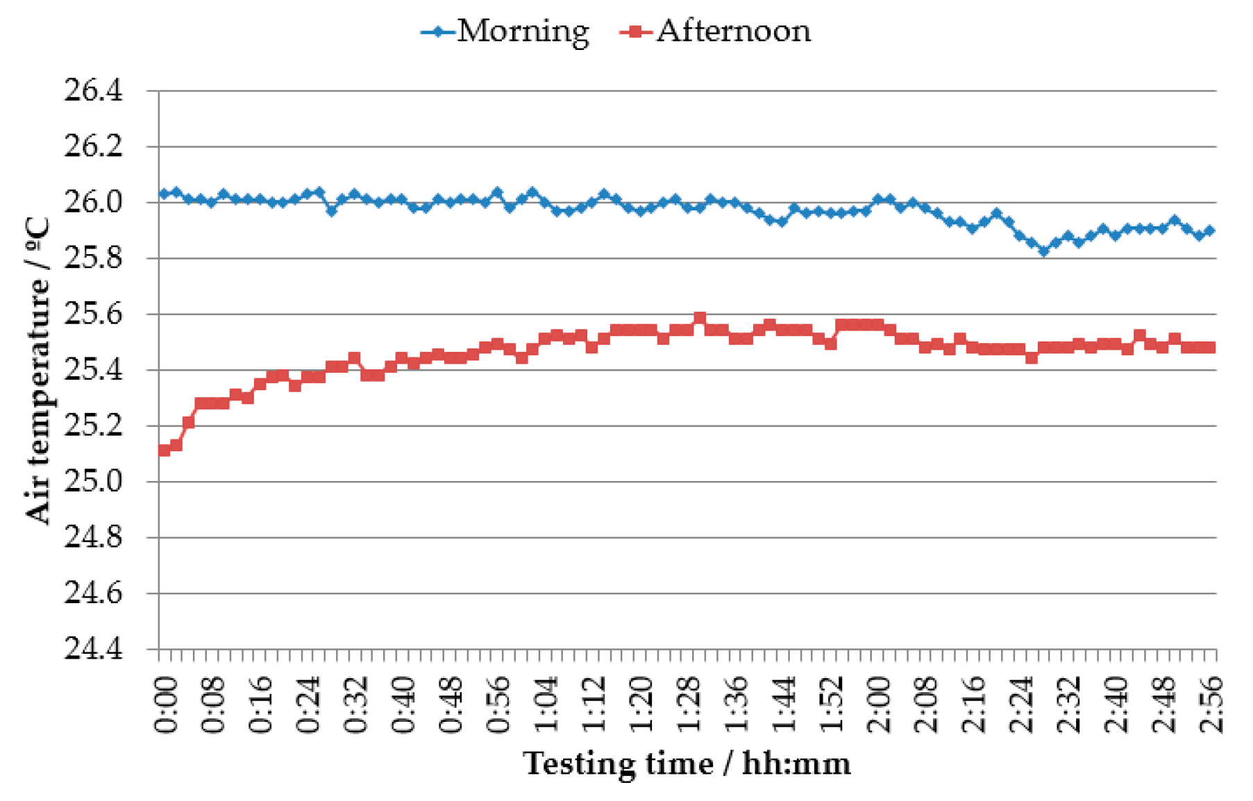
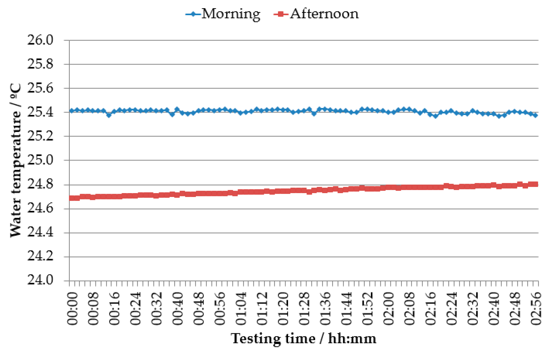
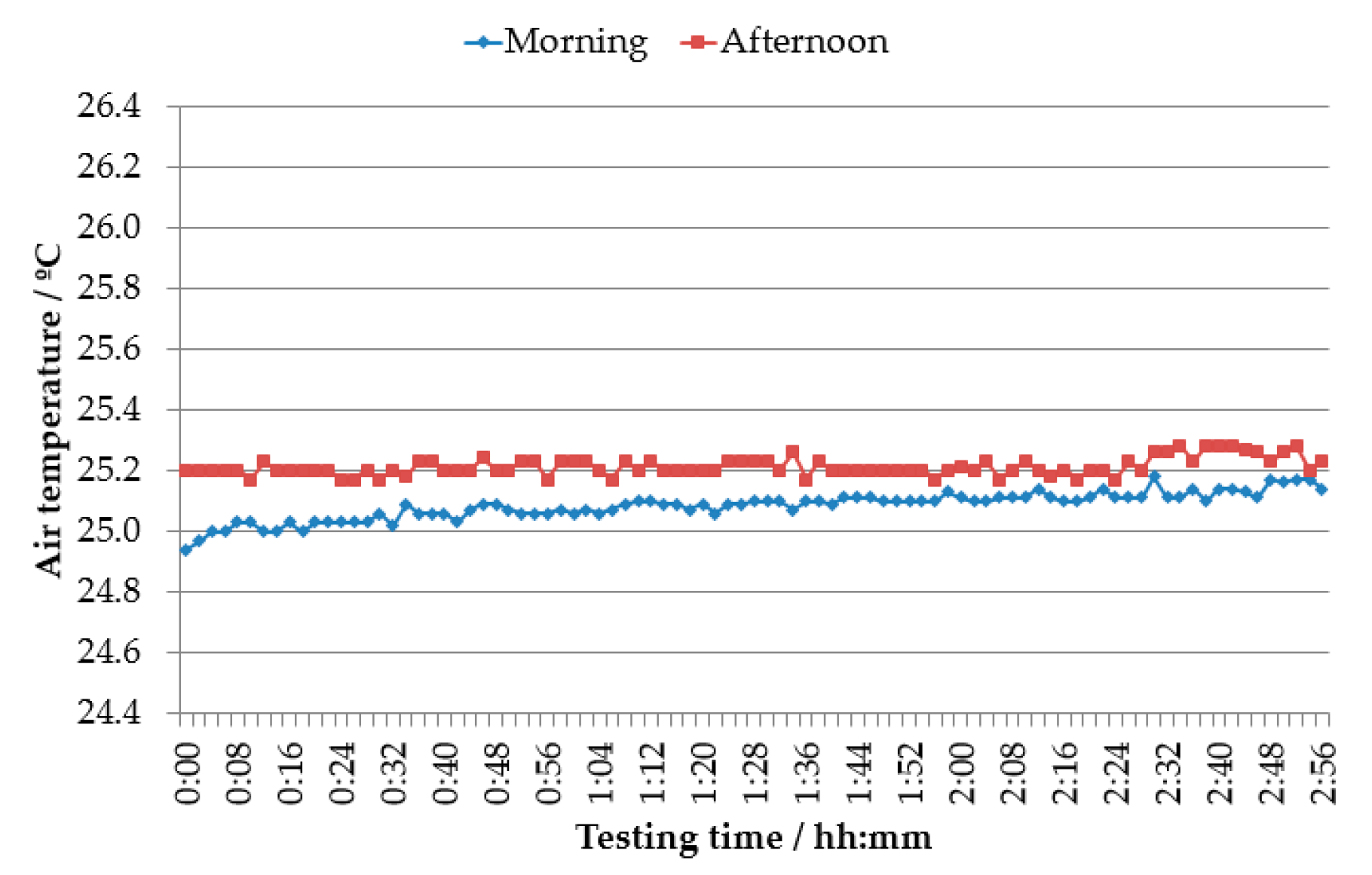
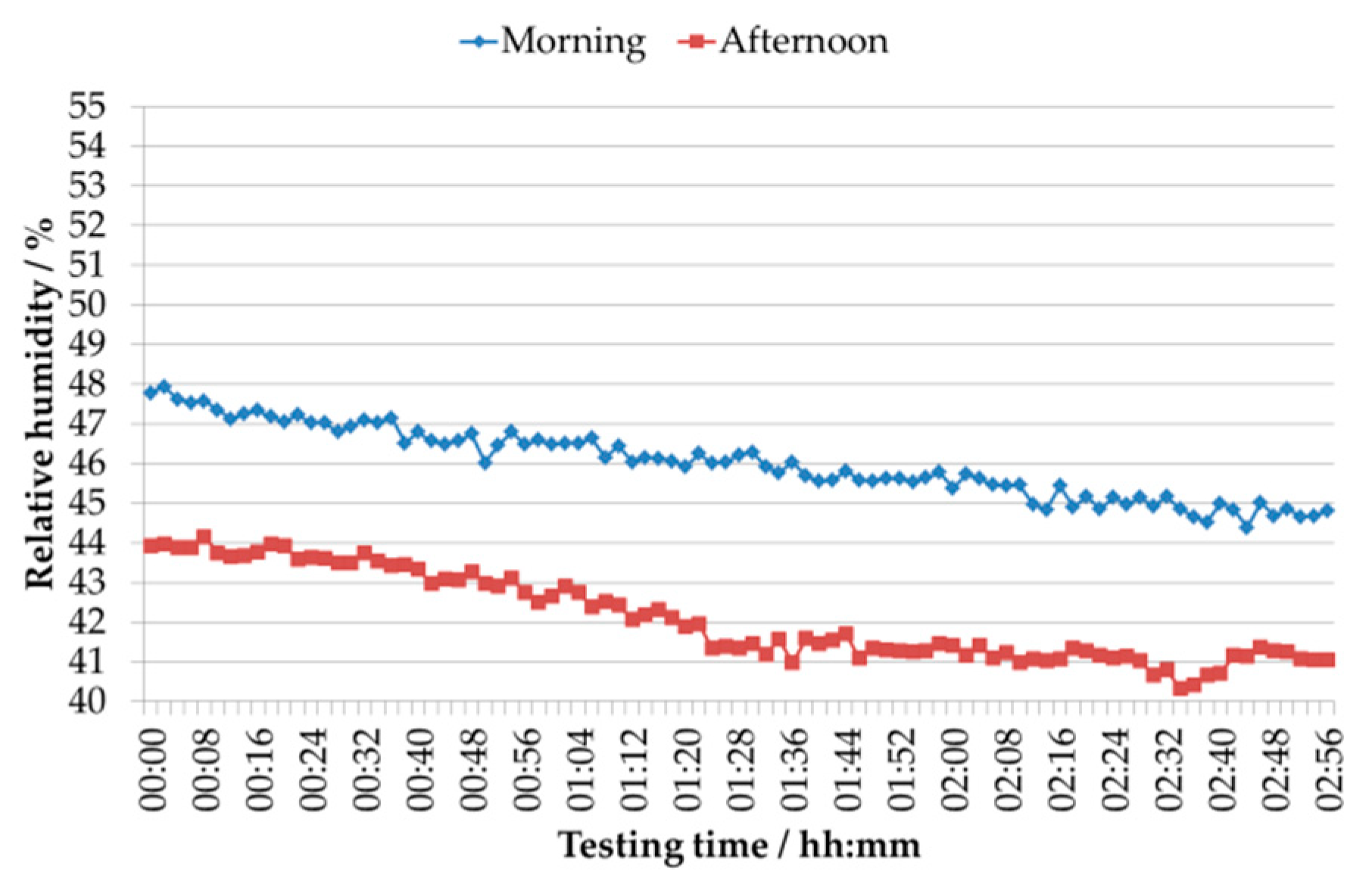
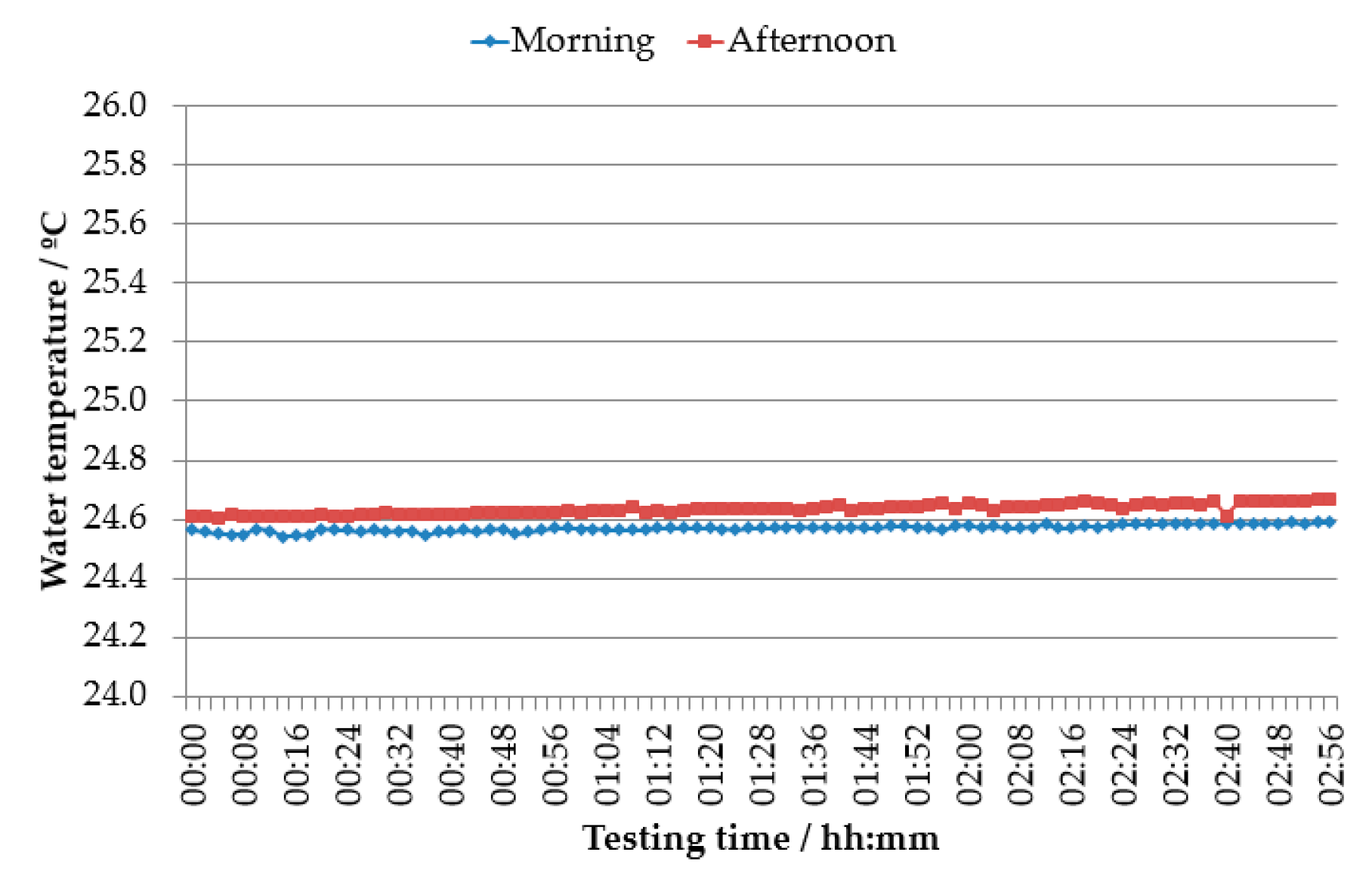
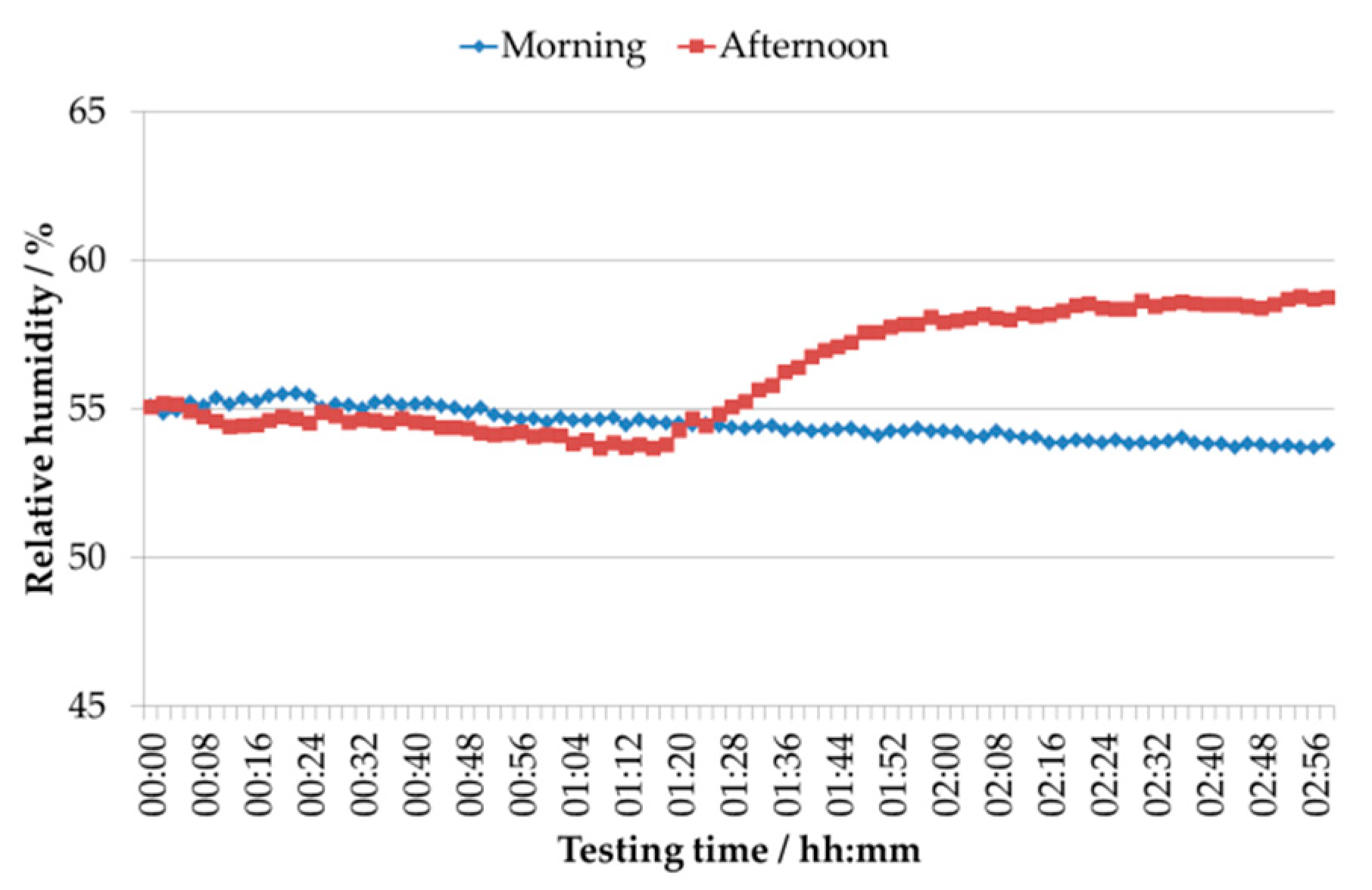
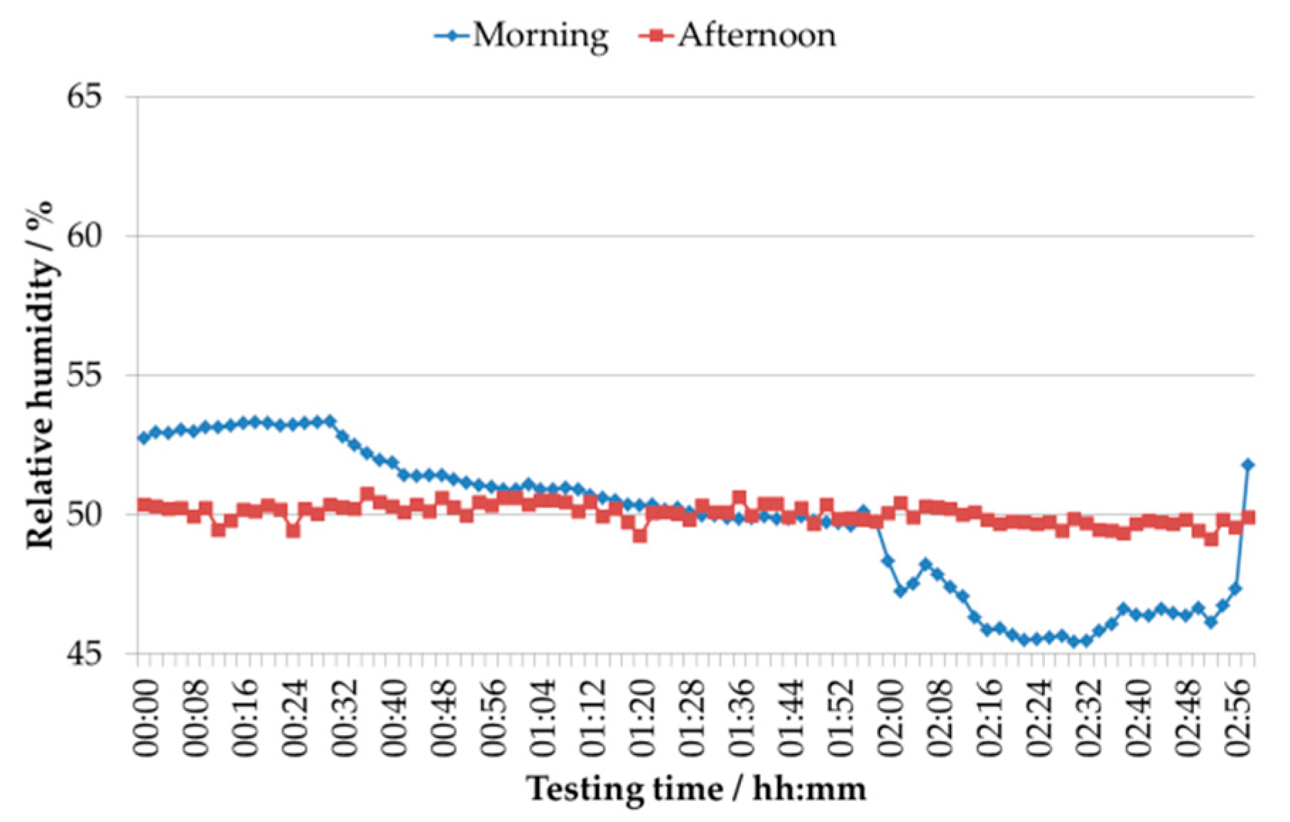
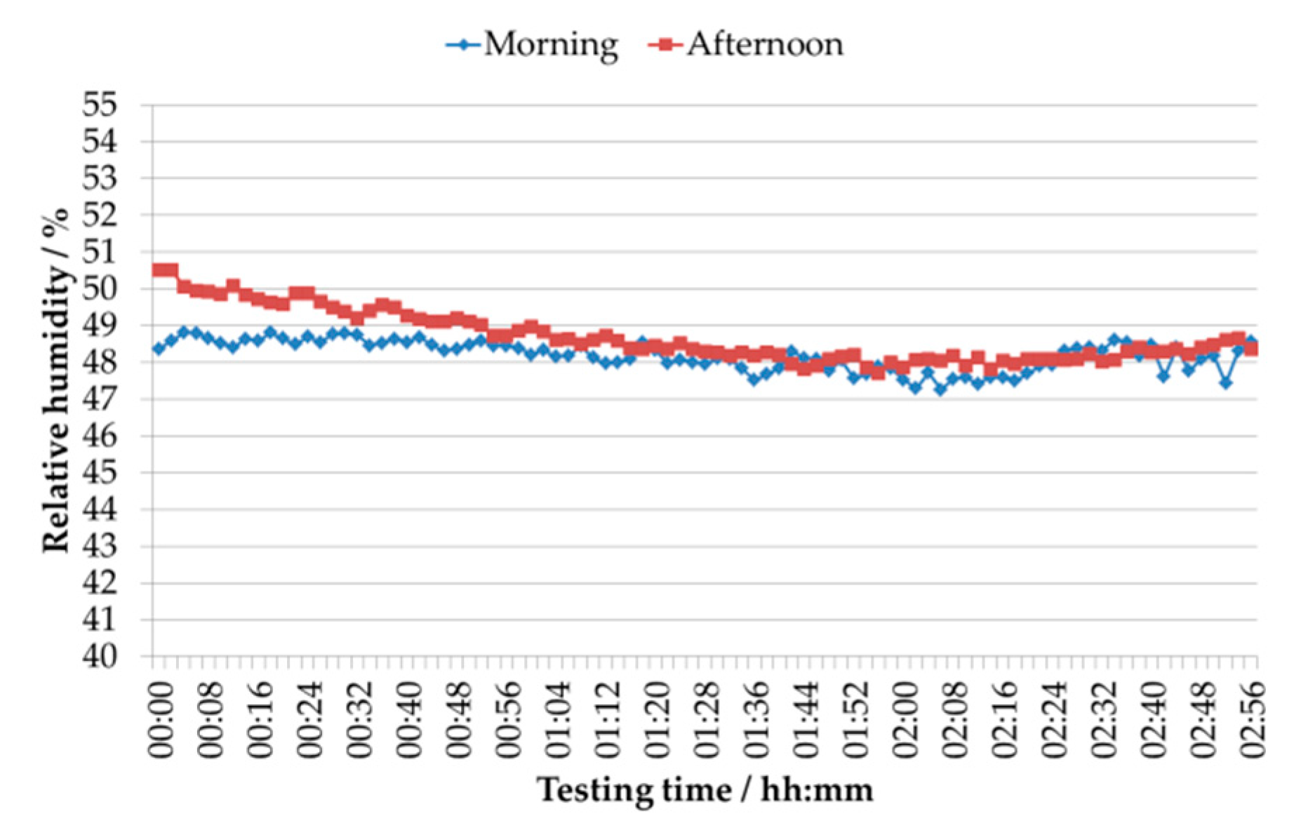
It should be noted that, the laboratorial testing of conductance transducers is performed in a controlled environment, which is significantly different from the application scenario of conductance transducers in maritime reduced-scale models, constructed in large experimental indoor infrastructures, where influence quantities, such as air temperature and relative humidity, water temperature, and electrical power supply, show a larger variation.

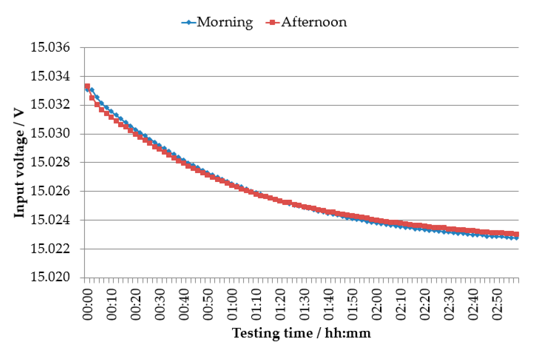
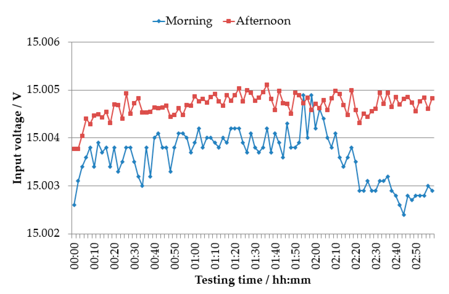
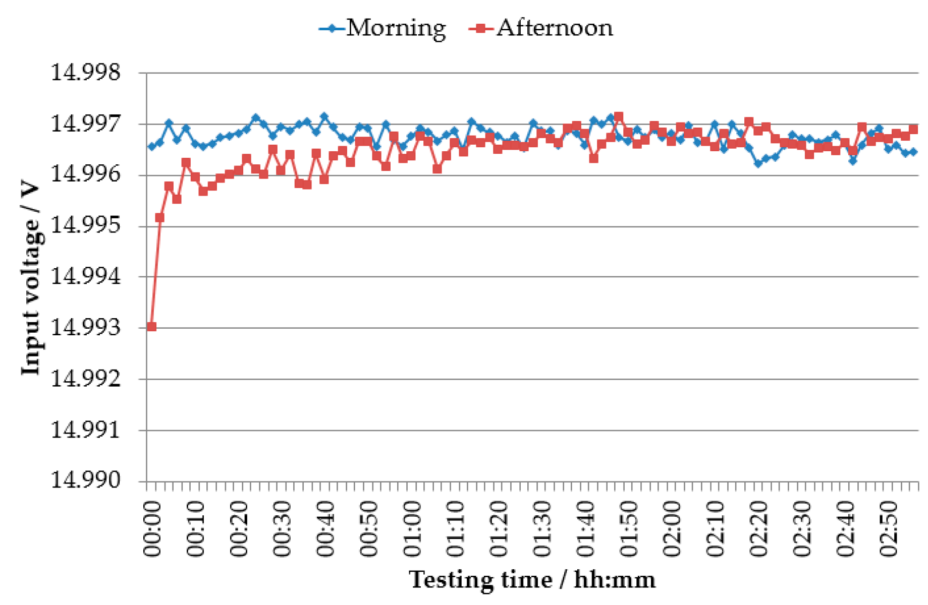
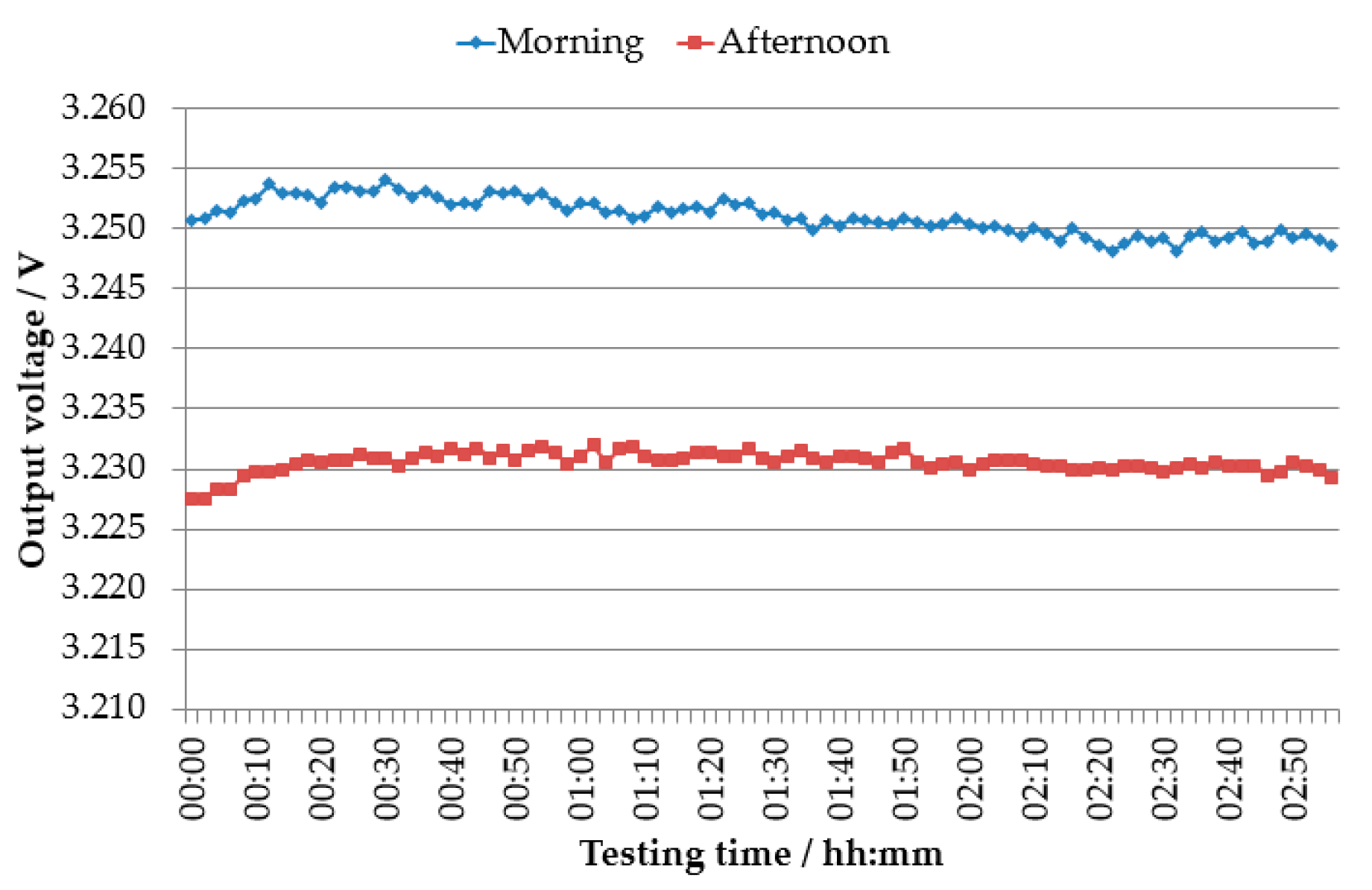
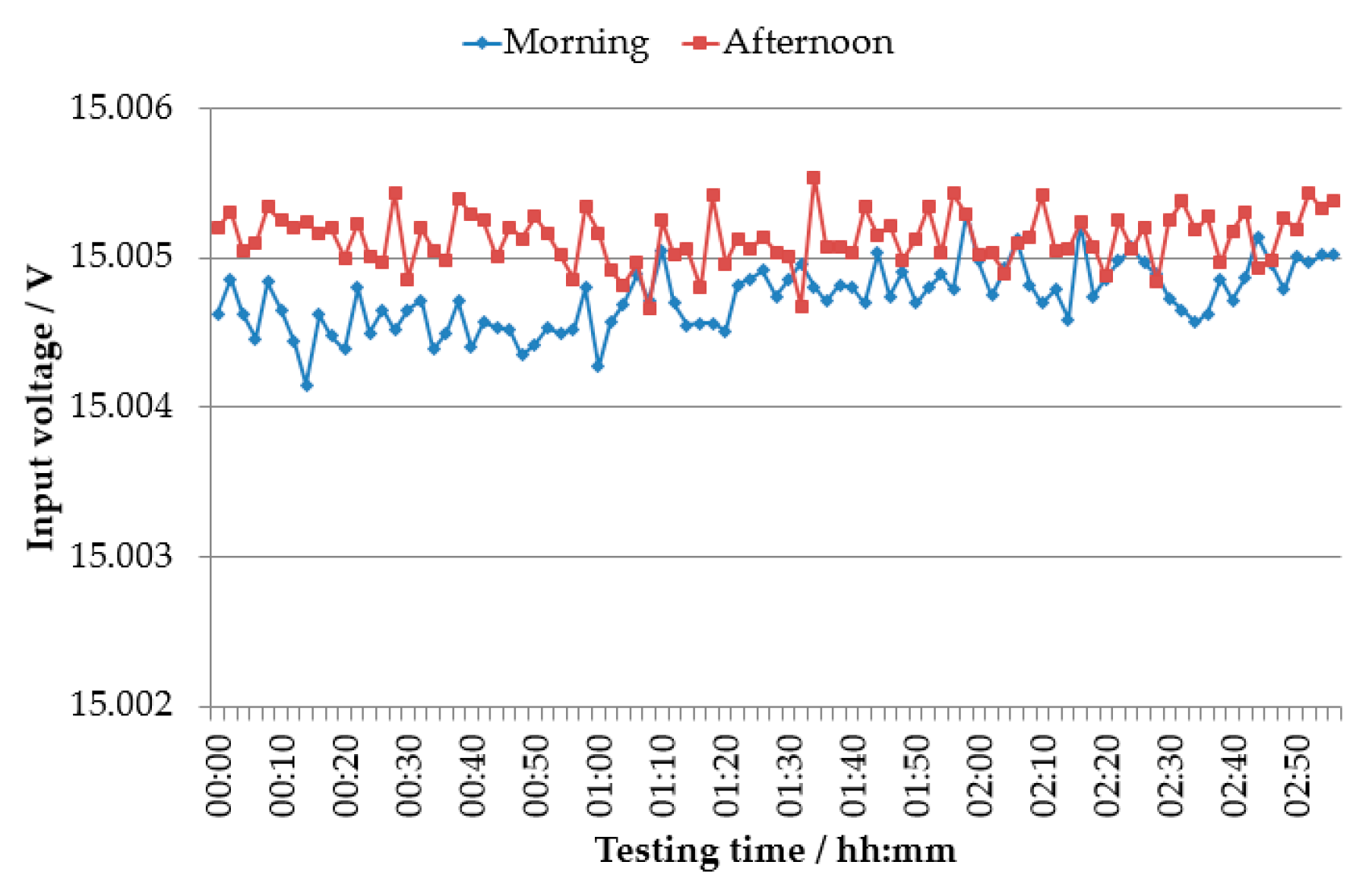
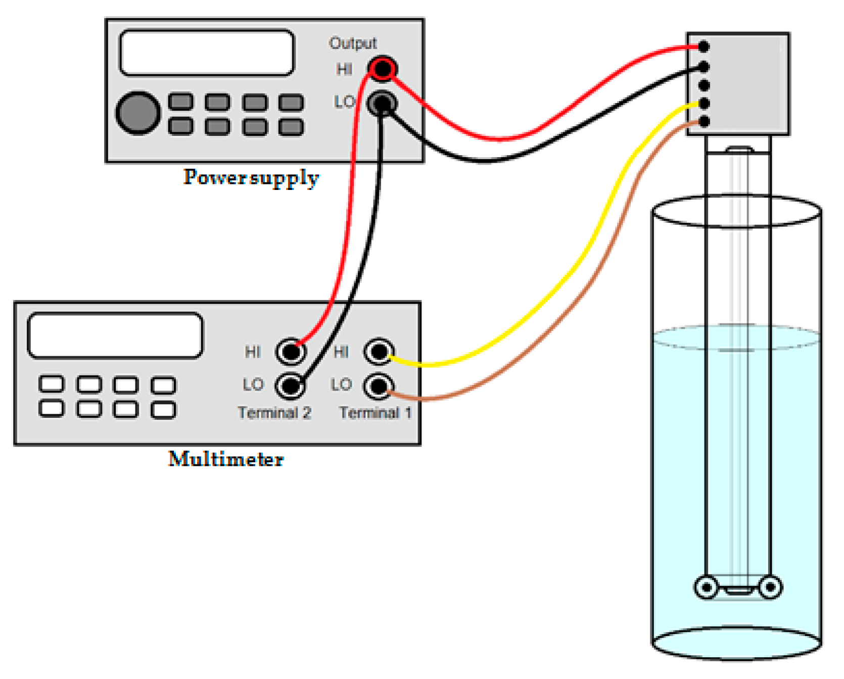
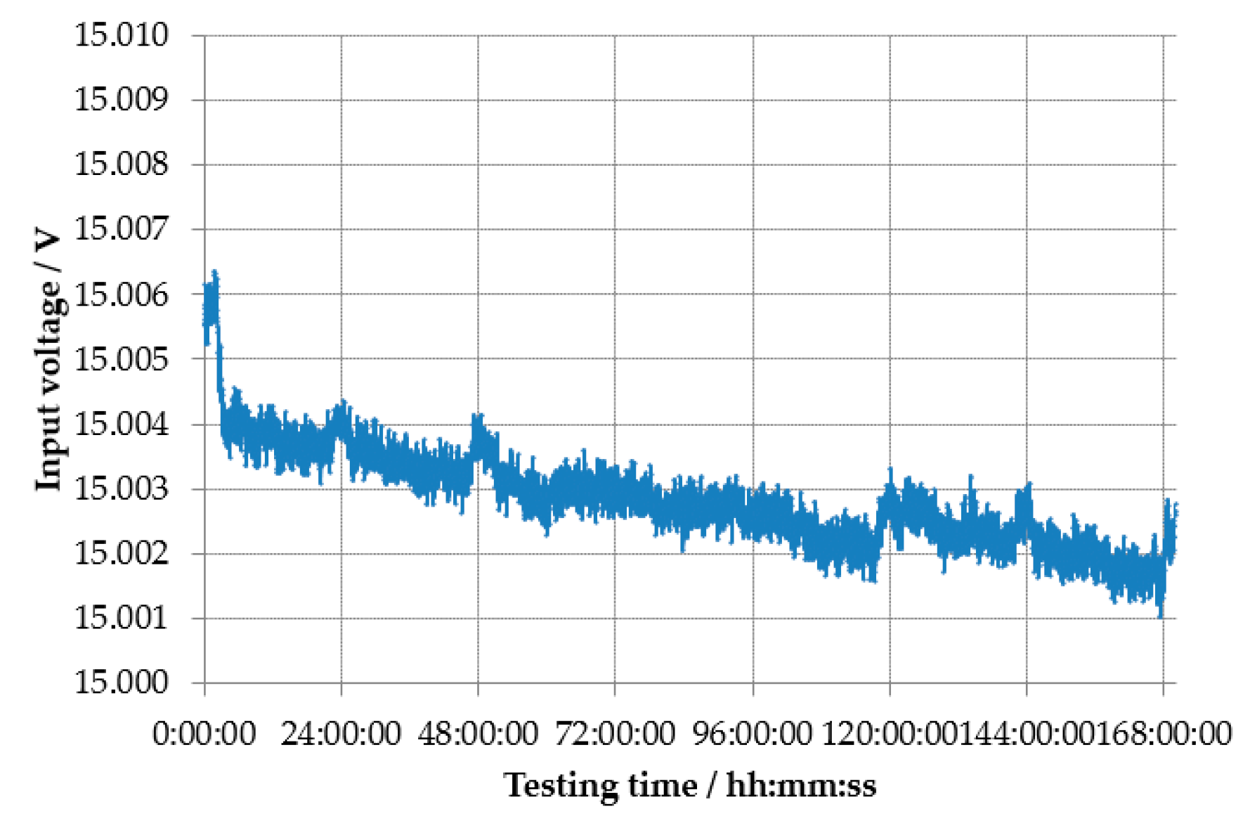
The characterization method of the electrical stability is divided in two parts: (i) power supply testing, in an empty condition (without connection to a conductance transducer) and a nominal input voltage set point of 15 V (DC); and (ii) the loaded condition test, where the same input voltage is applied to a conductance transducer, in a fixed half-immersion position in water, as schematically represented in Figure 2.

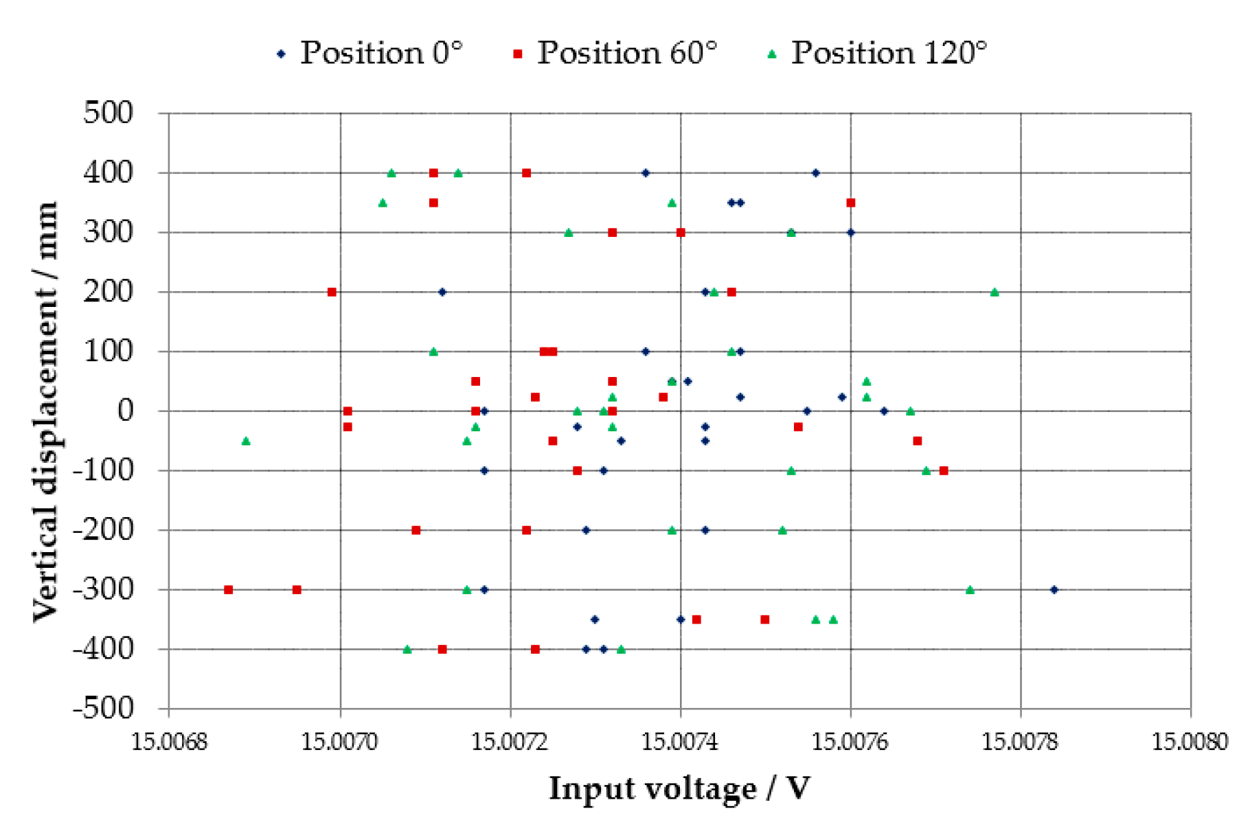
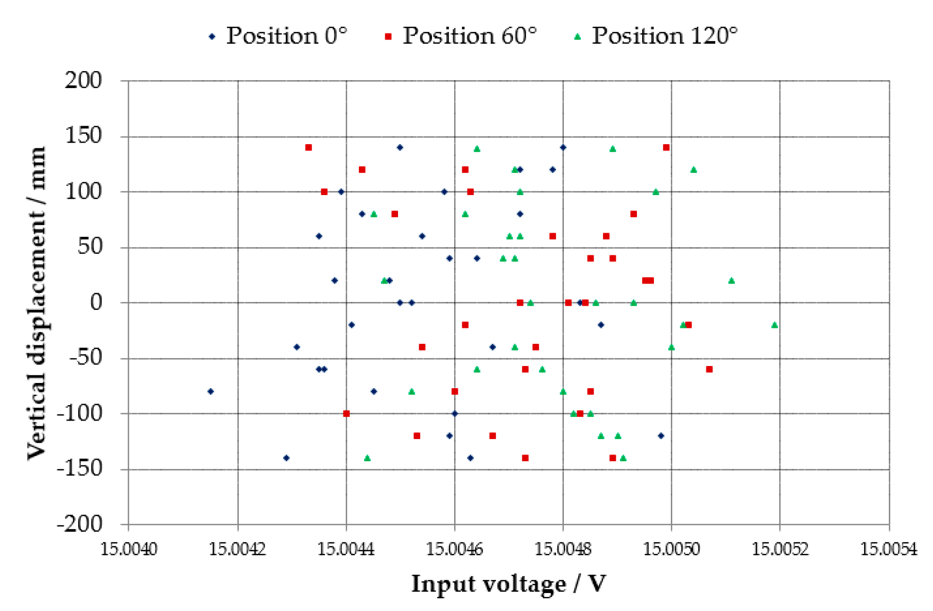
These tests were performed with two power supplies: (i) an off-the-shelf power supply (Agilent, model U8001A, Santa Clara, CA, USA), used for the testing of conductance transducers at laboratory; and (ii) a custom-made power supply (design and produced by LNEC), used for quality control and maintenance activities. The loaded condition test was performed for two conductance transducers (LNEC, internal reference id’s 54.12 and 57.12) with different measurement intervals, respectively, ±400 mm, and ±140 mm.

For each test, a three-hour duration was defined, and the voltage (input voltage in both the empty and the loaded condition tests, and the output voltage only in the loaded condition test) were measured considering an acquisition time period of two minutes, using a digital multimeter (HP, model 3457A). The tests were performed in the same laboratorial facility used to determine the conductance transducers linearity, reversibility, and repeatability (described in Section 3.2). Air temperature and relative humidity measurements were performed with a digital thermohygrometer recorder (Rotronic, model Hygrolog), while the water temperature in the loaded condition test was obtained from a resistance thermometer and a Wheatstone bridge (ASL, model F250). These measurements were performed simultaneously with the voltage measurements above mentioned.

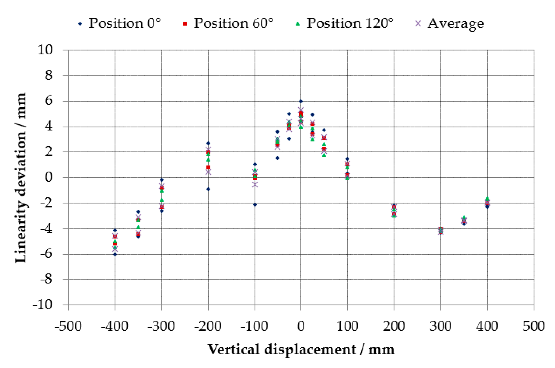
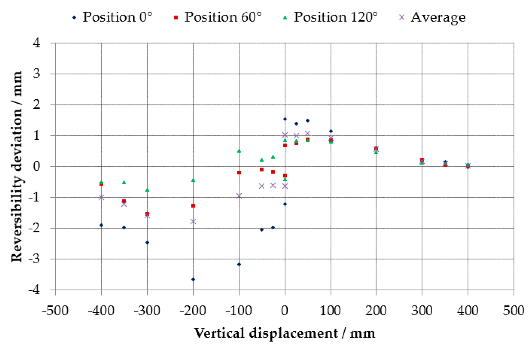
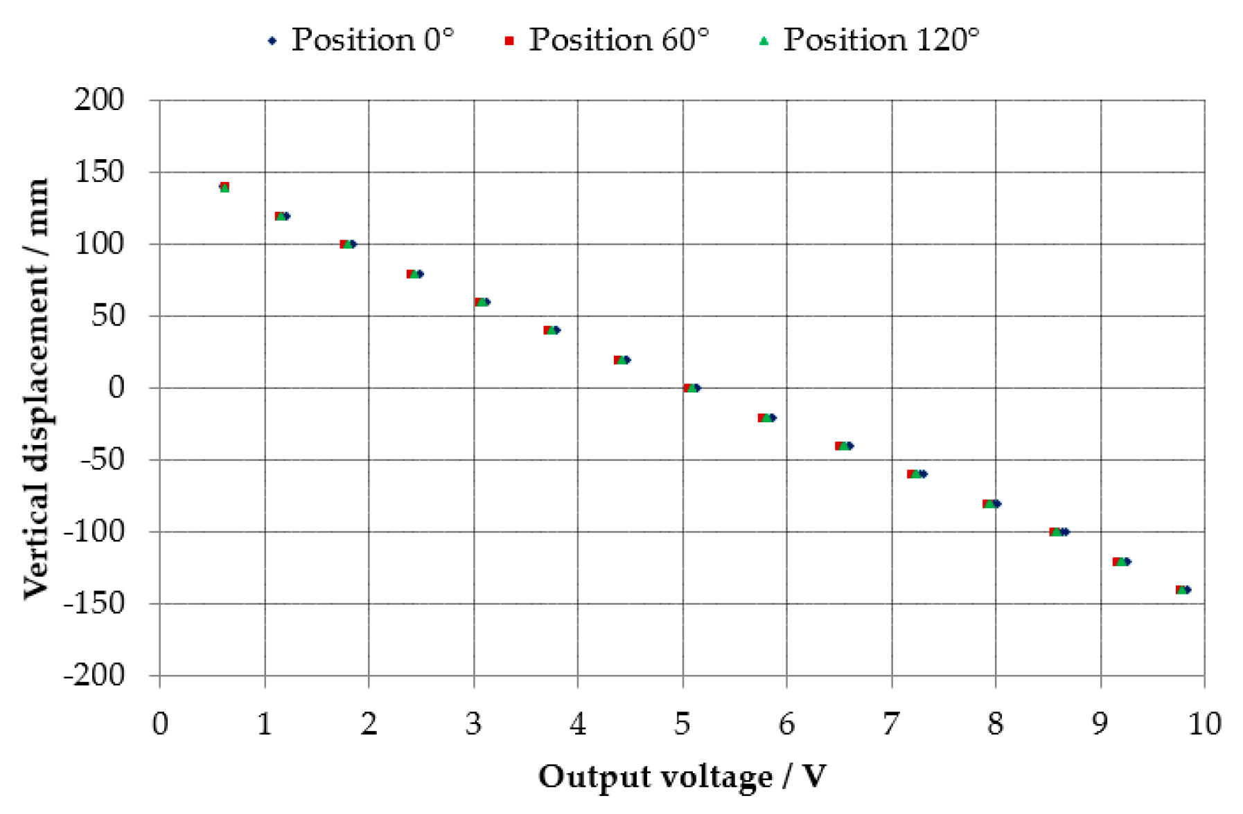
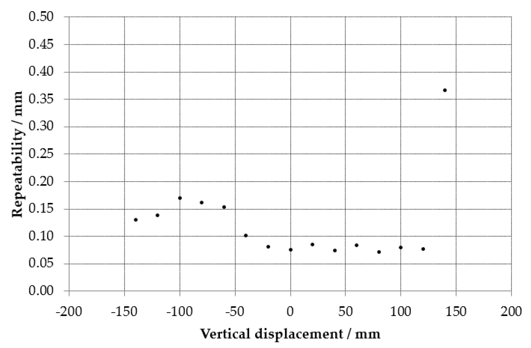
3.2. Linearity, Reversibility, and Repeatability

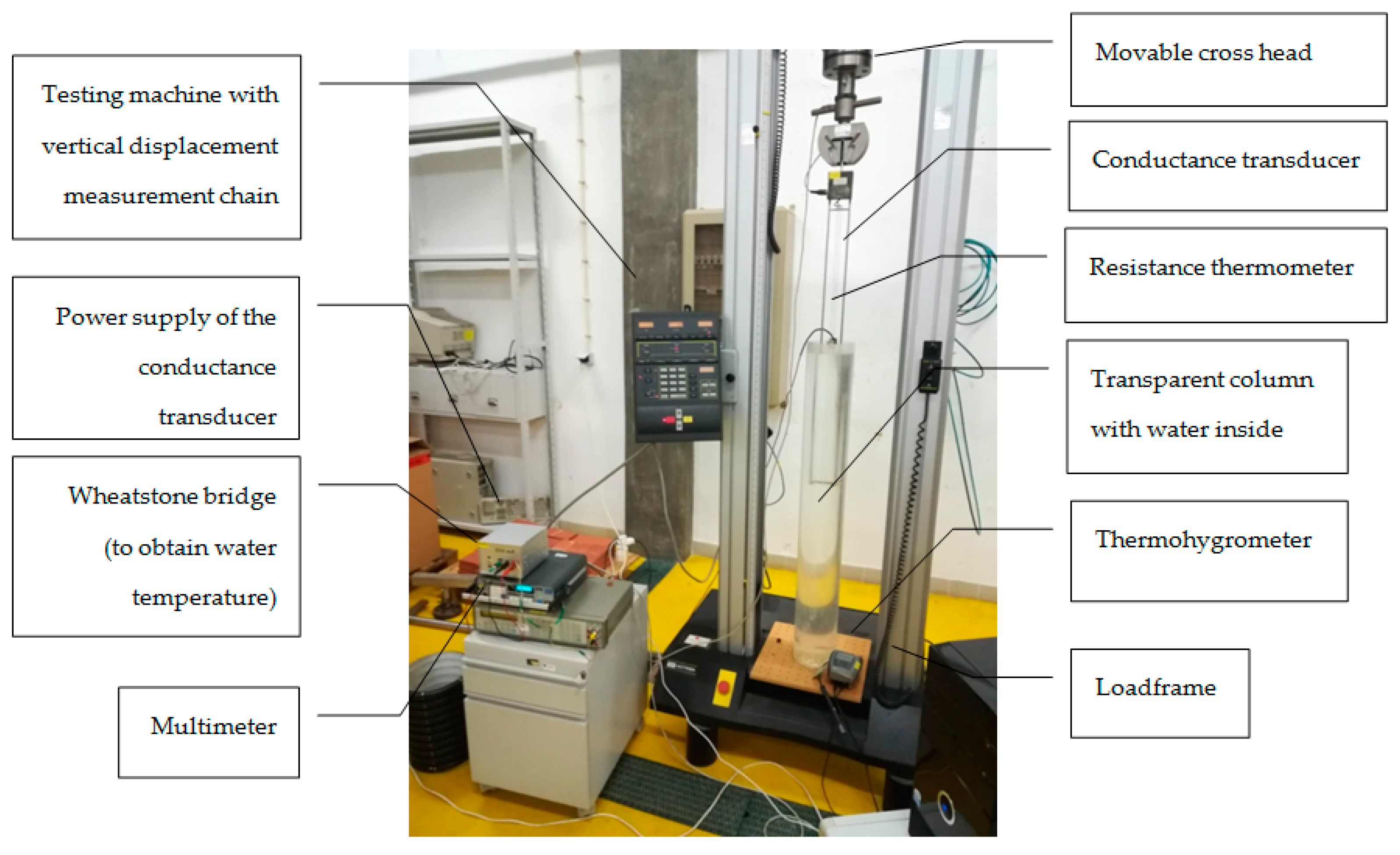
The characterization method proposed for the determination of the conductance transducers linearity, reversibility, and repeatability consists in the application of vertical unidirectional displacement steps to the tested transducer, which is immersed in water inside a transparent column. The experimental implementation of this method requires the use of a universal testing machine with a displacement range close to 2 m (as shown in Figure 3), noticing that some of the LNEC’s conductance transducers can have high vertical length.

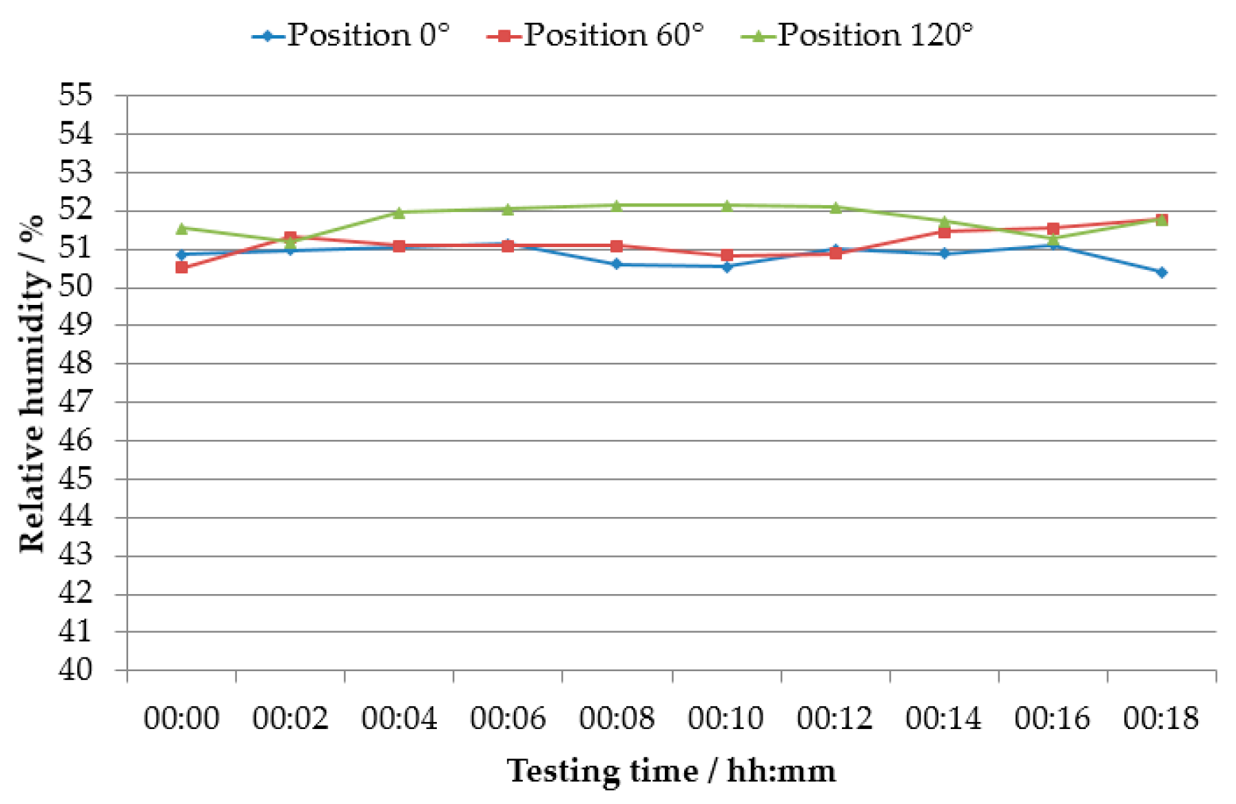
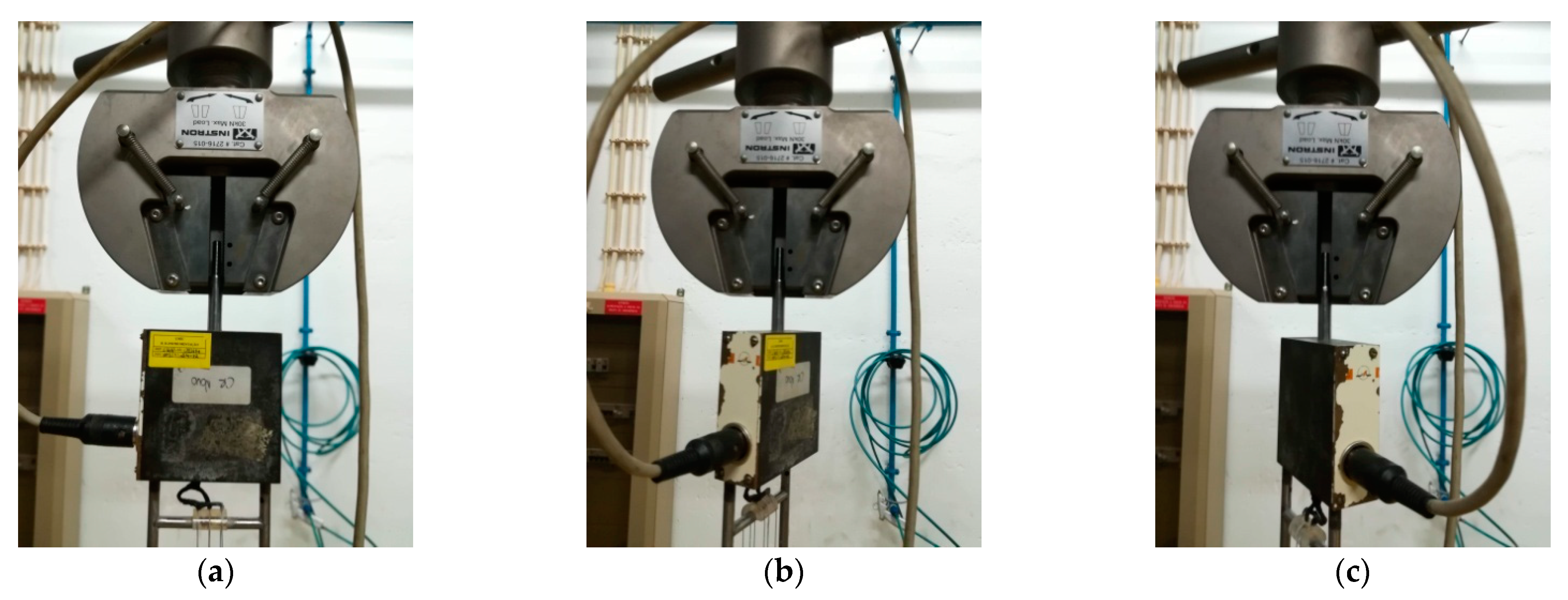
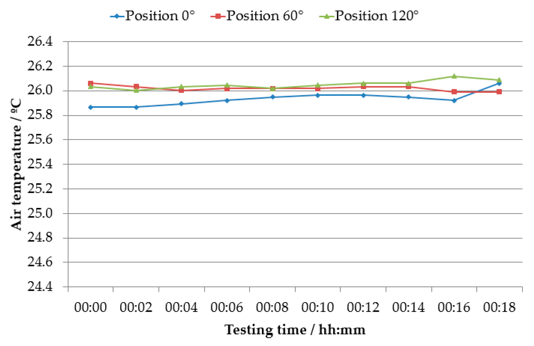
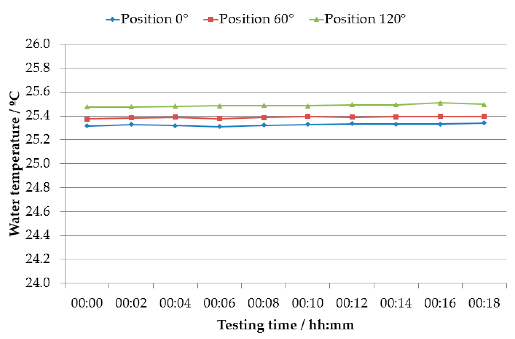
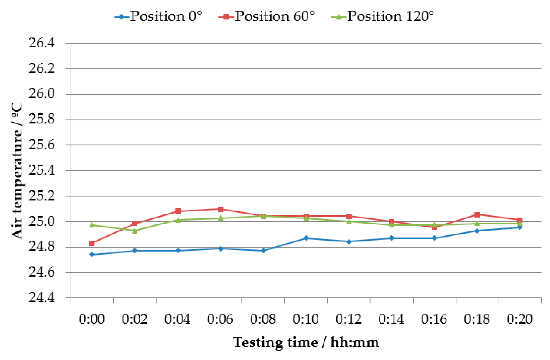
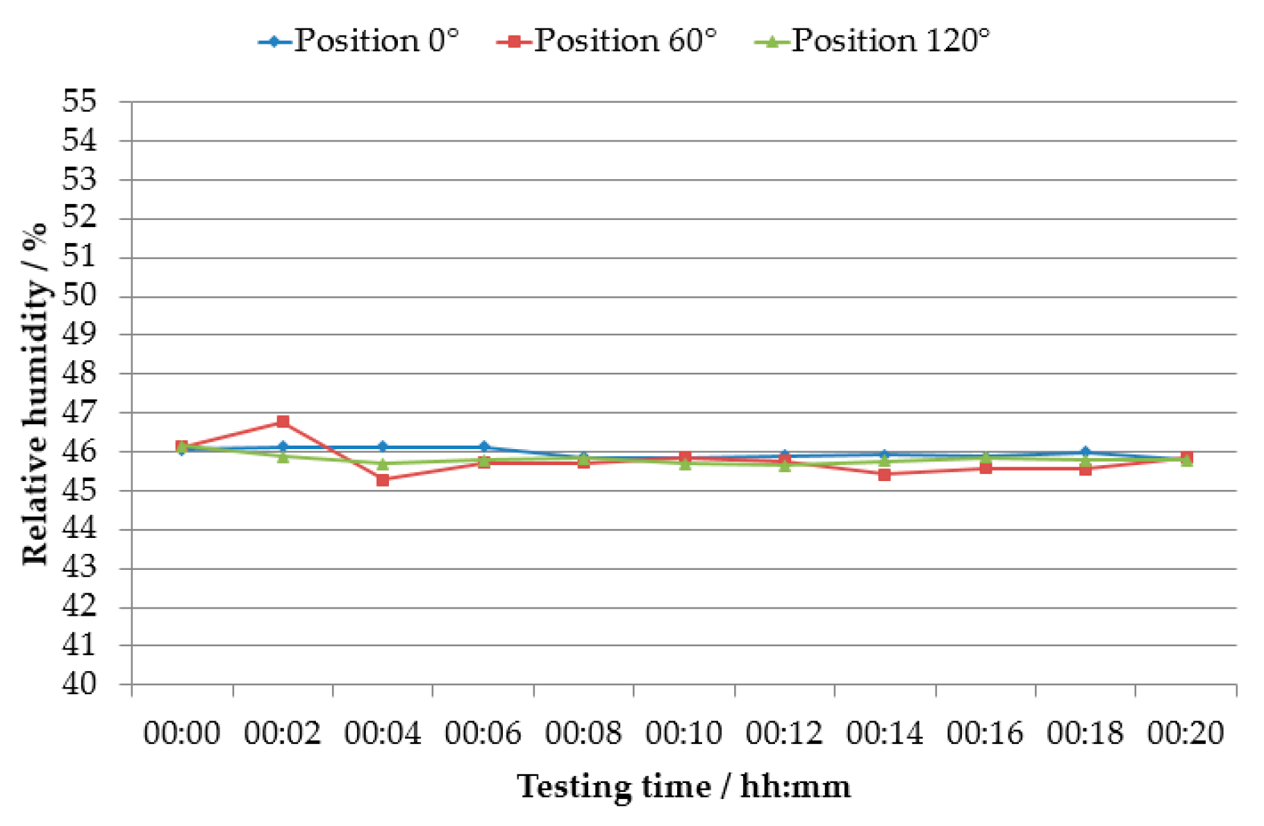
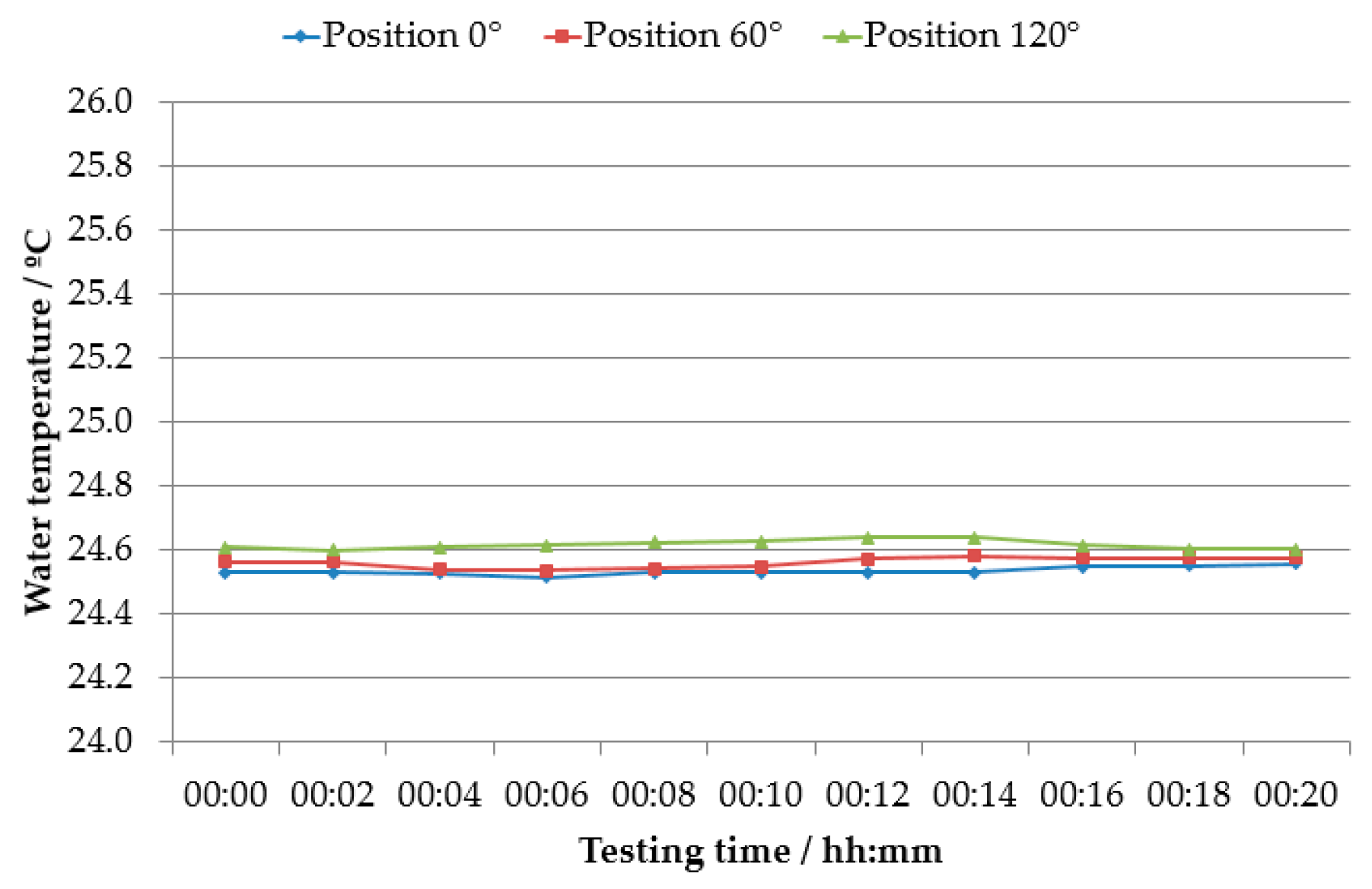
The conductance sensor top end-point can be mechanically fixed to the movable cross head of the testing machine and inserted inside the transparent column, which is installed in the lower region of the load frame. In order to reduce the perpendicularity deviation of the sensor relative to the water surface, namely in the case of high magnitude displacements, the test should be performed three times, applying a rotation of, approximately, 60° relative to the vertical axis between consecutive tests, as shown in Figure 4.

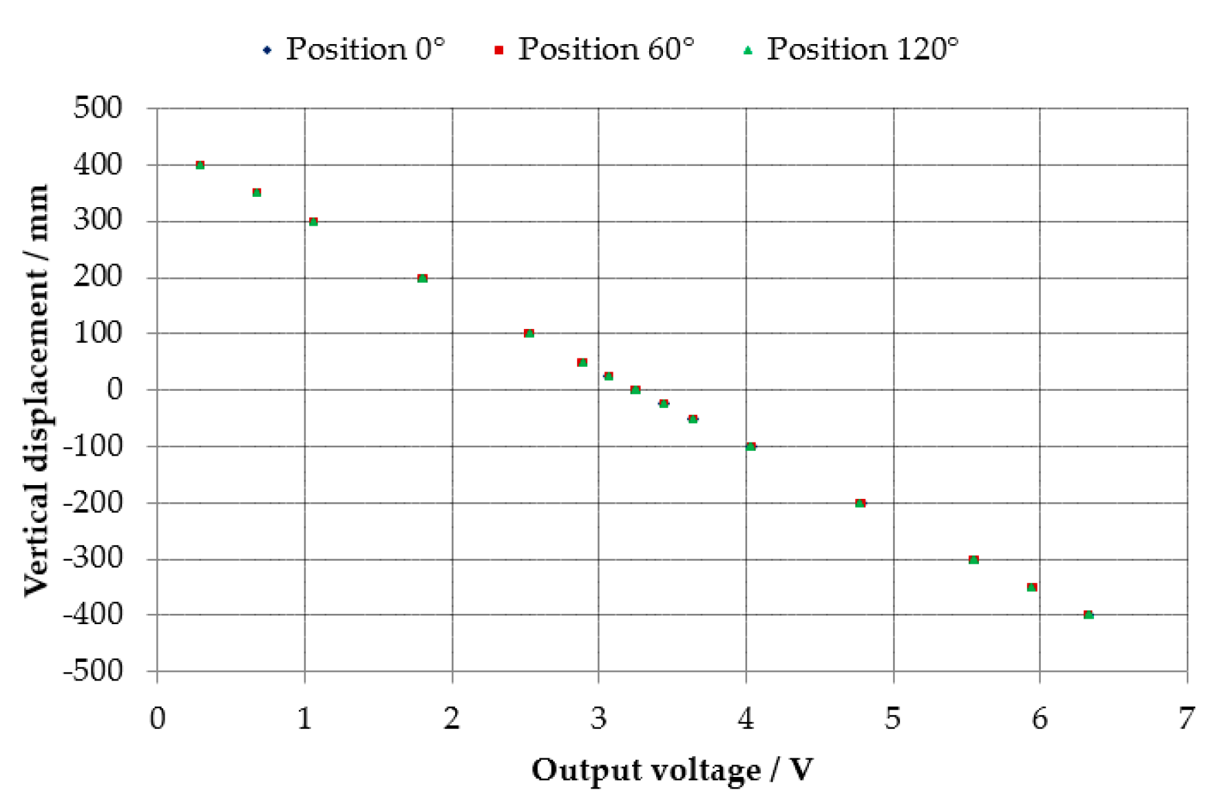
In these tests, the applied displacement to the conductance transducer is assumed as negative in the downward direction, while displacement in the upward direction is considered positive. The first testing step (considered as the zero reference for displacement) corresponds to the half-immersion position of the transducer in the water. In addition to this initial setting, a total of 30 displacement steps equally distributed in the transducer measurement range was applied, considering the following sequence: (i) a downward cycle, starting from the zero position up to the transducer’s upper water level threshold; (ii) an upward cycle, from the transducer’s upper water level threshold to its lower water level threshold, passing by the zero position; (iii) a downward cycle, returning from the lower water level threshold to the zero position.

This characterization method was applied to the two previously mentioned (see Section 3.1) conductance transducers (with measurement intervals of ±400 mm and ±140 mm) and power supply, regulated for an input voltage equal to 15 V (DC).In each testing step, both the input and the output voltage of the transducer are measured with a digital multimeter (already mentioned in Section 3.1), in addition to the displacement quantity obtained from the dimensional measuring chain of the testing machine (Instron, model 4467). Air temperature and relative humidity and water temperature measurements are performed in a similar way, as mentioned in Section 3.1.

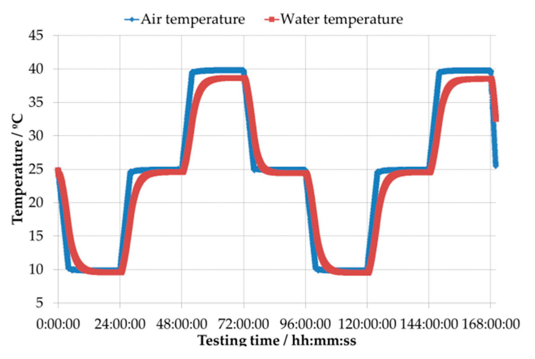
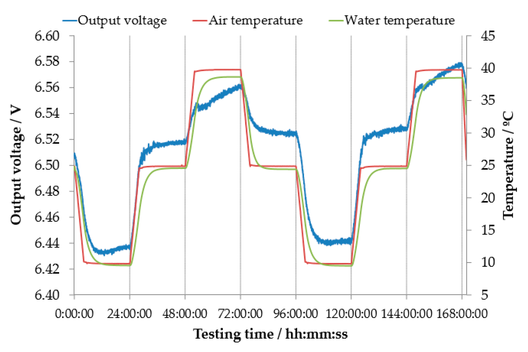
3.3. Thermal Influence

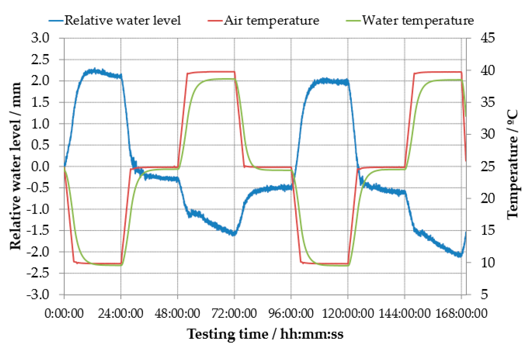
The characterization of the thermal influence on conductance transducers is considered a relevant condition to be studied, namely in the temperature interval ranging from 10 °C up to 40 °C, since maritime reduced-scale models are usually tested in large experimental indoor facilities where the air temperature can easily reach these extreme values between winter and summer seasons.

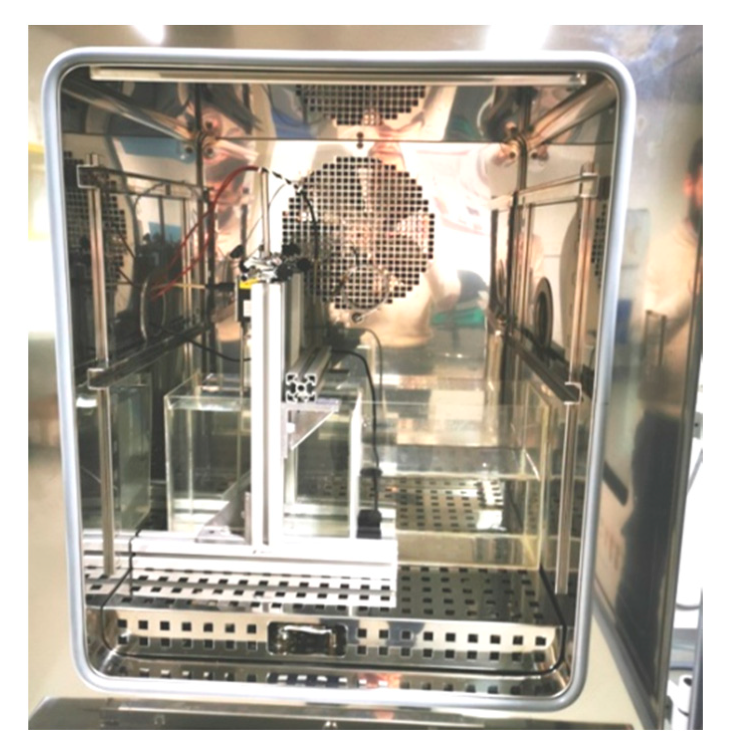
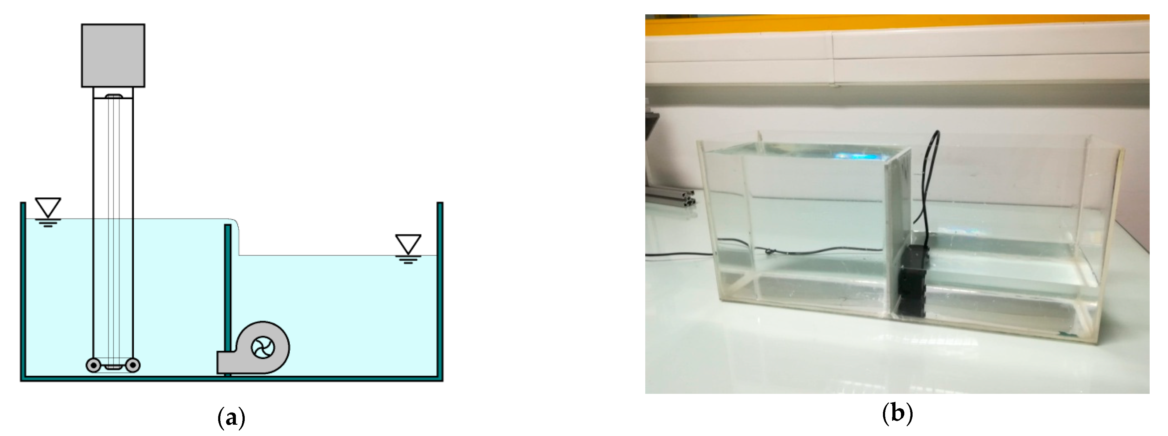
The proposed characterization method is supported in the use of a climatic chamber, where a conductance sensor can be installed, having half-immersion position at the water level. Due to the evaporation phenomenon, the water level can be significantly reduced, namely, if long-term thermal testing is made. In order to maintain a constant water level in the testing box of the conductance transducer, a water reservoir prototype was designed and produced, being composed by two separated compartments, being the water circulation between the compartments assured by a system of a propeller connected to an electrical engine, as seen in Figure 5.

The established hydraulic circuit originates different, but nearly stationary, water levels in each compartment. One of them is used for the conductance transducer immersion, while the remaining one contains the propeller and the electrical engine.

In this study, due to the volume restriction inside the climatic chamber (Aralab, model Fitoclima 300, with known thermal stability and uniformity), this assembly was applied to the thermal testing of a conductance transducer (id. 57.12) with a measurement interval of ±140 mm, connected to the studied off-the-shelf power source, regulated for a nominal input voltage of 15 V (DC). Water and air temperature measurements were obtained from two resistance thermometers connected to a Wheatstone bridge (ASL, model F250) and installed, respectively, in the water compartment of the conductance transducer and in the climatic chamber, as shown in Figure 6.

The thermal cycle setup in the climatic chamber was composed by the following air temperature sequence: 10 °C; 25 °C; 40 °C; 25 °C; 10 °C; 25 °C; 40 °C. Each of the mentioned testing steps had a duration of 20 h with a transition ramp of four hours between steps; therefore, the total duration of the thermal testing corresponded to 172 h. For these temperatures, input and output voltages were measured at conductance transducer terminals (using a digital multimeter HP, model 3457A) having a sampling rate for all the measured quantities of two minutes between consecutive measurements.

4. Experimental Results

4.1. Electrical Stability

4.1.1. Empty Condition

The electrical stability of the two available power supplies—custom-made and off-the-shelf—was evaluated in the empty condition (without a connection to a conductance transducer and in same laboratory room where the linearity and reversibility tests were later on performed), during three hours in both morning and afternoon periods. The recorded input electrical voltage is shown in Figure 7 and Figure 8, respectively, for the custom-made and the off-the-shelf power supplies. The air temperature and relative humidity records are presented in Appendix A.

Significant differences are noticed between the two tested power supplies. The custom-made power supply shows an input voltage that converges from an initial value of 15.033 V to a final value of 15.023 V, while the input voltage related to the off-the-shelf power supply remains approximately stable, with a variation in time below 1 mV. Based on the obtained results, the off-the-shelf power supply was used in the remaining electrical, dimensional, and thermal tests.

4.1.2. Loaded Condition

The electrical stability test in the loaded condition was performed following the procedure described in Section 3.1, in the same laboratory room where the dimensional tests were implemented later on. The off-the-shelf power supply was used and connected to two conductance transducers (±400 mm long-range transducer and a ±140 mm short-range transducer), each one tested twice (a first test in afternoon and a second test the following morning).

Figure 9 and Figure 10 show, respectively, the obtained input and output voltages of the long-range conductance transducer, while Figure 11 and Figure 12 correspond to the short-range conductance transducer results. The environmental records (air temperature, relative humidity, and water temperature) obtained in these tests are presented in Appendix B.

As seen in Figure 9 and Figure 11, the input voltage remained stable in time, close to the nominal value of 15 V, and with variation below 1 mV, maintaining a similar electrical behavior as observed previously in the empty condition test of the off-the-shelf power supply.

The output voltage records show a short-term initial transient behavior (approximately 15 min), where the output voltage increases, followed by a voltage step (during one hour) and then starts a slow descent in time. This output voltage decrease reflects the water evaporation phenomenon since, according to transducer’s measurement principle (explained in Section 2), a water level decrease is reflected in a related decrease of the output voltage.

4.1.3. Environmental Stability

The electrical tests performed also allow evaluating the environmental conditions of the laboratory room, previously to the dimensional tests of the conductance transducers. Taking into account the environmental records shown in Appendix A, the laboratory room is characterized by a stable air temperature with a variation below 0.2 °C in a three- hour period. It also shows a reduce level of relative humidity (lower than 65%) with a maximum variation of 5%. The water temperature showed a more stable behavior (close to 0.1 °C), when compared with the air temperature, due to its higher thermal inertia. In particular, the water temperature records show a linear increase of its magnitude as a result of the Joule effect in the transducer’s electrodes and consequent heat transfer to the water.

4.2. Linearity, Reversibility, and Repeatability

4.2.1. Long-Range Conductance Transducer (±400 mm)

The conductance transducer with a measurement interval of ±400 mm was tested, following the proposed method for the determination of linearity, reversibility, and repeatability, using the off-the-shelf power supply. During the performed tests, the average air temperature was comprised between 25.8 °C and 26.1 °C, while the relative humidity varied between 50% and 52%. The water temperature was slightly lower than the air temperature, with a minimum value of 25.3 °C and a maximum value equal to 25.5 °C. Figure 13 and Figure 14 show the applied vertical displacement relative to the recorded input and output voltage, respectively, while Figure 15, Figure 16 and Figure 17 represent the obtained linearity and reversibility deviations and repeatability, respectively, as a function of the output voltage.

Figure 13 shows that the input voltage remained stable during the test, varying between 15.0068 V and 15.0078 V, without showing correlation with the applied vertical displacement (random distribution of the experimental values for all the testing positions).

With respect to the output voltage, a linear relation with the applied vertical displacement is observed in Figure 14, for the voltage measurement interval between 0.2 V and 6 V, with no significant differences between test positions. Based on these results, Figure 15 presents the corresponding linearity deviations, which can reach a maximum absolute value close to 6 mm, considering a measurement interval of ±400 mm. These deviations show a non-random behavior, indicating that a linear calibration curve is a first approximation to the relation between the output voltage and the applied vertical displacement. In the negative part of the dimensional measurement interval, the dispersion of linearity deviation values is higher when compared to the positive region.

This can be justified by reversibility, as shown in Figure 16, where the average absolute value is close to 2 mm, while in the positive region the average reversibility has a maximum value near 1 mm. A detailed observation of Figure 16 shows that reversibility deviations are mainly due to the results of the first performed test (position 0°), obtained for negative displacements from the half-immersion position to the full-immersion position. This shows the influence of the dry or wet condition of the transducer electrodes in the performed tests, since the first test (position 0°) is the only one, which starts with the half-length electrodes in a dry condition. In the remaining consecutive tests (positions 60° and 120°), the electrodes are already wet in their full-length; therefore, improving the transducer’s reversibility.

The transducer’s repeatability (see Figure 17) is also affected by the reversibility results, having its best value in the positive region (0.05 mm), while in the negative region, the repeatability varies between 0.25 and 0.55 mm, reflecting the measurement uncertainty source related to the wet or dry condition of the electrodes during the tests.

Table 1. Estimates and standard uncertainties of the calibration curve linear parameters related to the long-range conductance transducer.

Linear Parameter	Test Position 0°	Test Position 60°	Test Position 120°	Average Position
Slope (mm∙V−1)	−132.94 ± 0.37	−133.03 ± 0.34	−132.96 ± 0.34	−132.98 ± 0.35
Intercept (mm)	436.2 ± 1.4	436.4 ± 1.3	436.3 ± 1.2	436.3 ± 1.3
Correlation factor	−0.88	−0.88	−0.88	−0.88

mentions, for each tested position and for the average results, the calculated linear parameters estimates, and standard uncertainties of the calibration curve between the output voltage and the applied displacement, obtained by the application of the Least Squares Method.

The results presented in Table 1 show minor differences between both the estimates and standard uncertainties of the linear parameters, for all the tested positions, noticing slightly higher uncertainties in the test position 0°, for the same reasons discussed before in this section. The magnitude of the difference between estimates, considering the same type of linear parameter for different test positions, is much lower that the obtained standard uncertainty level, indicating reduce perpendicularity deviations between the transducer’s electrodes and the water surface.

The correlation factor between the linear parameters was equal to −0.88, showing that the linear calibration curve can be taken as a first approximation to the relation between the output voltage and the vertical displacement (the correlation factor between parameters in a theoretic linear relation is equal to one).

4.2.2. Short-Range Conductance Transducer (±140 mm)

The conductance transducer with a measurement interval of ±140 mm was tested, following the proposed method for the determination of linearity, reversibility, and repeatability, using the off-the-shelf power supply. During the performed tests, the average air temperature was comprised between 24.7 °C and 25.1 °C, while the relative humidity varied between 45% and 47%. The water temperature was slightly lower than the air temperature, with a minimum value of 24.5 °C and a maximum value equal to 24.7 °C. Figure 18 and Figure 19 show the applied vertical displacement relative to the recorded input and output voltages, respectively, while Figure 20, Figure 21 and Figure 22 represent the obtained linearity and reversibility deviations and repeatability, respectively, as a function of the output voltage.

Figure 18 shows that the input voltage remained stable during the performed test, varying between 15.0041 and 15.0052 V, with no signs of correlation with the applied vertical displacement (random distribution of the experimental values for all the testing positions).

With respect to the output voltage, a linear relation with the applied vertical displacement is observed in Figure 19, for the voltage measurement interval between 0.5 and 10 V, with no significant differences between test positions. Based on these results, Figure 20 presents the corresponding linearity deviations, showing a cyclical variation between 2 and −4 mm, considering a measurement interval of ±140 mm. In the same way as the case of the long-range transducer (see Figure 15 in Section 4.2.1), this systematic behavior shows that the linear calibration curve is a first approximation to the relation between the output voltage and the applied vertical displacement. The highest linearity deviation was obtained in the 60° test position, for the extreme positive vertical displacement, which is close to the transducer’s operational limit.

With respect the reversibility results (shown in Figure 21), the same cyclical variation seen in the linearity deviations, is also noticed but with a reduced magnitude, close (in average) to ±0.5 mm. The highest reversibility absolute deviations (near 1 mm) were obtained in the first tested position (0°), confirming the influence of the wet or dry electrodes condition in the obtained results, as seen in the case of the long-range transducer (see Section 4.2.1).

The transducer’s repeatability (see Figure 22) is also affected by the reversibility results, having its best value in the positive region, below 0.10 mm (ignoring the result obtained for the extreme positive vertical displacement, close to the transducer’s operational limit).In the negative region, the repeatability reaches a maximum value of 0.17 mm, reflecting the measurement uncertainty source related to the wet or dry condition of the electrodes during the tests.

Table 2. Estimates and standard uncertainties of the calibration curve linear parameters related to the short-range conductance transducer.

Linear Parameter	Test Position 0°	Test Position 60°	Test Position 120°	Average Position
Slope (mm∙V−1)	−29.67 ± 0.13	−29.79 ± 0.15	−29.75 ± 0.12	−29.74 ± 0.13
Intercept (mm)	154.36 ± 0.77	152.82 ± 0.85	153.35 ± 0.74	153.51 ± 0.78
Correlation factor	−0.88	−0.87	−0.88	−0.88

mentions, for each tested position and for the average results, the calculated linear parameters estimates, and standard uncertainties of the calibration curve between the output voltage and the applied displacement, obtained by the application of the Least Squares Method.

The results presented in Table 2 show minor differences between both the estimates and standard uncertainties of the linear parameters, for all the tested positions, noticing slightly higher uncertainties in the test position 60°, which can reflect the effect of some perpendicularity deviation between the transducer’s electrodes and the water surface in this position. This was also noticed in the corresponding correlation factor (further away from the theoretical unitary value).

The average correlation factor between the linear parameters was equal to −0.88 (the same value obtained for the long-range conductance transducer, see Table 1), confirming the linear calibration curve has a first approximation to the relation between the output voltage and the vertical displacement.

4.3. Thermal Influence

The experimental setup allowed applying controlled temperature steps to the conductance transducer, half-immersed in a constant water level. Figure 23 shows the obtained water and air temperature time evolutions, while

Table 3. Average and experimental standard deviation values related to the last 30 min of the temperature testing steps.

Temperature Set Point/°C	Water Temperature/°C	Air Temperature/°C	Temperature Difference between Air and Water/°C
10	9.555 ± 0.001	9.833 ± 0.003	0.278
25	24.567 ± 0.001	24.869 ± 0.003	0.302
40	38.640 ± 0.001	39.773 ± 0.002	1.133
25	24.397 ± 0.001	24.872 ± 0.003	0.475
10	9.505 ± 0.001	9.820 ± 0.003	0.315
25	24.528 ± 0.001	24.866 ± 0.003	0.338
40	38.515 ± 0.001	39.737 ± 0.003	1.222

presents the average and the experimental standard deviation values of the last 30 min of each temperature step.

Figure 23 shows convergent steps for both the air and water temperatures, noticing a faster evolution of the air temperature during transitions due to the higher thermal inertia of water. Each temperature step also shows high temperature stability, as seen in Table 3, for the last 30 min of each temperature step (experimental standard deviation values of 0.001 °C and 0.003 °C, respectively, for the water and the air temperatures). However, the comparison between the average values mentioned in Table 3 shows temperature differences between water and air, ranging from 0.278 °C up to 1.222 °C. Temperature differences are particularly high in the 40 °C temperature step, being the air temperature always higher than the water temperature.

During the thermal test of the conductance transducer, the input voltage applied by the power supply was recorded and is shown in Figure 24.

As shown in Figure 24, during the thermal test a variation of 5.4 mV was observed—corresponding to the difference between the maximum (15.0064 V) and the minimum (15.0010 V) recorded input voltage values—noticing a decreasing evolution from an initial stage to the end of the test. An abrupt decrease in the input voltage was noticed after three hours, which can be attributed to a transient warming period of the used electrical equipment. After this, the input voltage evolution maintained its decreasing linear tendency in time, showing reduced magnitude peaks in its profile during transitions between temperature steps. This electrical signal was characterized by an approximately constant noise close to 0.2 mV, after removing the linear tendency.

With respect to the output voltage of the conductance transducer, Figure 25 shows its time evolution during the performed thermal test, in addition to the previously shown air and water temperature records (in Figure 23). The corresponding average and experimental standard deviation values of both the input and output voltage are mentioned in

Table 4. Input and output average voltage and experimental standard deviation values related to the last 30 min of the temperature testing steps.

Temperature Set Point/°C	Input Voltage/V	Output Voltage/V
10	15.0039 ± 0.0001	6.4377 ± 0.0008
25	15.0037 ± 0.0002	6.5177 ± 0.0013
40	15.0030 ± 0.0002	6.5610 ± 0.0007
25	15.0026 ± 0.0001	6.5244 ± 0.0009
10	15.0028 ± 0.0002	6.4417 ± 0.0012
25	15.0026 ± 0.0002	6.5283 ± 0.0008
40	15.0016 ± 0.0002	6.5778 ± 0.0008

, considering the last 30 min of the temperature testing steps.

Figure 25 shows convergent output voltage values for each temperature step, with the exception of the 40 °C temperature step, where an increasing linear (long-term) tendency is observed. This voltage behavior can be justified by: (i) the high temperature environment increases water electrolysis and polarization effects in the metallic electrodes, which are reflected in a higher electrical current and, therefore, in a higher output voltage; (ii) a more significant thermal vertical stratification of the water temperature (with the contribution of the high magnitude—above 1 °C—temperature difference between water and air temperature at the 40 °C testing step), making the application of the horizontal electrode less effective in the compensation of water resistivity variation by the thermal effect, noticing that this compensation electrode is located in a lower region of the conductance transducer.

A transient voltage behavior is noticed in the beginning of each temperature step, similar to the transient thermal behavior of the air and water temperatures. Short-term stationary regimes, related to the last 30 min of the temperature testing steps, are characterized by an electrical stability of the output voltage equal or below 1.3 mV.

Both Figure 25 and Table 4 show that a temperature decrease originates a decrease in the output voltage and reciprocally, reflecting a higher or lower electrical current between the vertical electrodes, assuming that variations in the water resistivity are properly compensated by the horizontal electrode. Output voltage reversibility is also noticed in each temperature step, namely, 4.0 mV at 10 °C, 10.6 mV at 25 °C and 16.8 mV at 40 °C (obtained from the output voltage values shown in Table 4 and expressed in absolute values), therefore, showing an increasing magnitude tendency with the temperature increase. This voltage behavior can be originated by an increasing and cumulative effect of water electrolysis in the transducer.

Using the average calibration linear parameters of the thermal tested conductance transducer (see Table 2, in Section 4.2.2), the output voltage profile can be converted to water level values, and a profile can be obtained, relative to the initial water level. A graphical representation of the calculated values is presented in Figure 26, while

Table 5. Relative water level average and experimental standard deviation values related to the last 30 min of the temperature testing steps.

Temperature Set Point/°C	Relative Water Level/mm
10	2.102 ± 0.004
25	−0.293 ± 0.007
40	−1.578 ± 0.004
25	−0.492 ± 0.005
10	1.968 ± 0.006
25	−0.608 ± 0.004
40	−2.077 ± 0.004

shows the dimensional conversion of Table 4.

The relative variation of the water level during the thermal test varied between a maximum value of 2.102 mm for the first 10 °C temperature step, and a minimum value of −2.077 mm for the last 40 °C temperature step. The above mentioned voltage stability is reflected in a dimensional variation equal or below 0.007 mm, while the dimensional reversibility corresponds to 0.134 mm at 10 °C, 0.199 mm at 25 °C, and 0.499 mm at 40 °C.

5. Instrumental Measurement Uncertainty

Based on the results obtained from the performed experimental activities described in Section 4, several uncertainty components were identified, each one contributing for the instrumental measurement uncertainty of the conductance transducer.

A first group of uncertainty components is related to the input quantities—output voltage and linear parameters of the calibration curve—which can be propagated to the output quantity—water level—by application of the GUM Law of Propagation of Uncertainty [9], resulting in the following expression:

$$u{\left(h\right)}_{\mathrm{cur}}=\sqrt{c_m^2·u^2\left(m\right)+c_V^2·u^2\left(V\right)+c_b^2·u^2\left(b\right)+2·c_m·c_b·u\left(m\right)·u\left(b\right)·r\left(m,b\right)}$$

(2)

taking into account the uncertainty contribution, u(h)_cur, of the adopted linear calibration curve of the conductance transducer

$$h=m·V+b,$$

(3)

where h is the water level (in mm), m is the slope linear parameter (expressed in mm∙V⁻¹), V is the output voltage of the conductance transducer (expressed in V) and b is the intercept linear parameter (in mm).

The sensitivity coefficients shown in Expression (2) are given by the following expressions:

$$c_m=\frac{\partial h}{\partial m}=V,$$

(4)

$$c_V=\frac{\partial h}{\partial V}=m,$$

(5)

$$c_b=\frac{\partial h}{\partial b}=1,$$

(6)

allowing to write Expression (3) as

$$u{\left(h\right)}_{\mathrm{cur}}=\sqrt{V^2·u^2\left(m\right)+m^2·u^2\left(V\right)+u^2\left(b\right)+2·V·u\left(m\right)·u\left(b\right)·r\left(m,b\right)}.$$

(7)

Both the standard uncertainties related to linear parameters, u(m) and u(b), as well as the correlation factor between parameters, r(m,b), can be obtained from the application of the Least Squares Method (examples shown in Table 1 and Table 2 of Section 4.2).

The standard uncertainty related to the output voltage, u(V), results from the combination of the identified uncertainty components: (i) calibration and drift of the used multimeter, u(V)_cal and u(V)_drf, respectively; (ii) resolution of the selected DC voltage measurement scale, u(V)_res; (iii) stability (noise) of the output voltage signal, u(V)_stb. Therefore, the application of the Law of Propagation of Uncertainty allows determining the standard uncertainty of the output voltage by

$$u\left(V\right)=\sqrt{u{\left(V\right)}_{\mathrm{cal}}^2+u{\left(V\right)}_{\mathrm{drf}}^2+u{\left(V\right)}_{\mathrm{res}}^2+u{\left(V\right)}_{\mathrm{stb}}^2}.$$

(8)

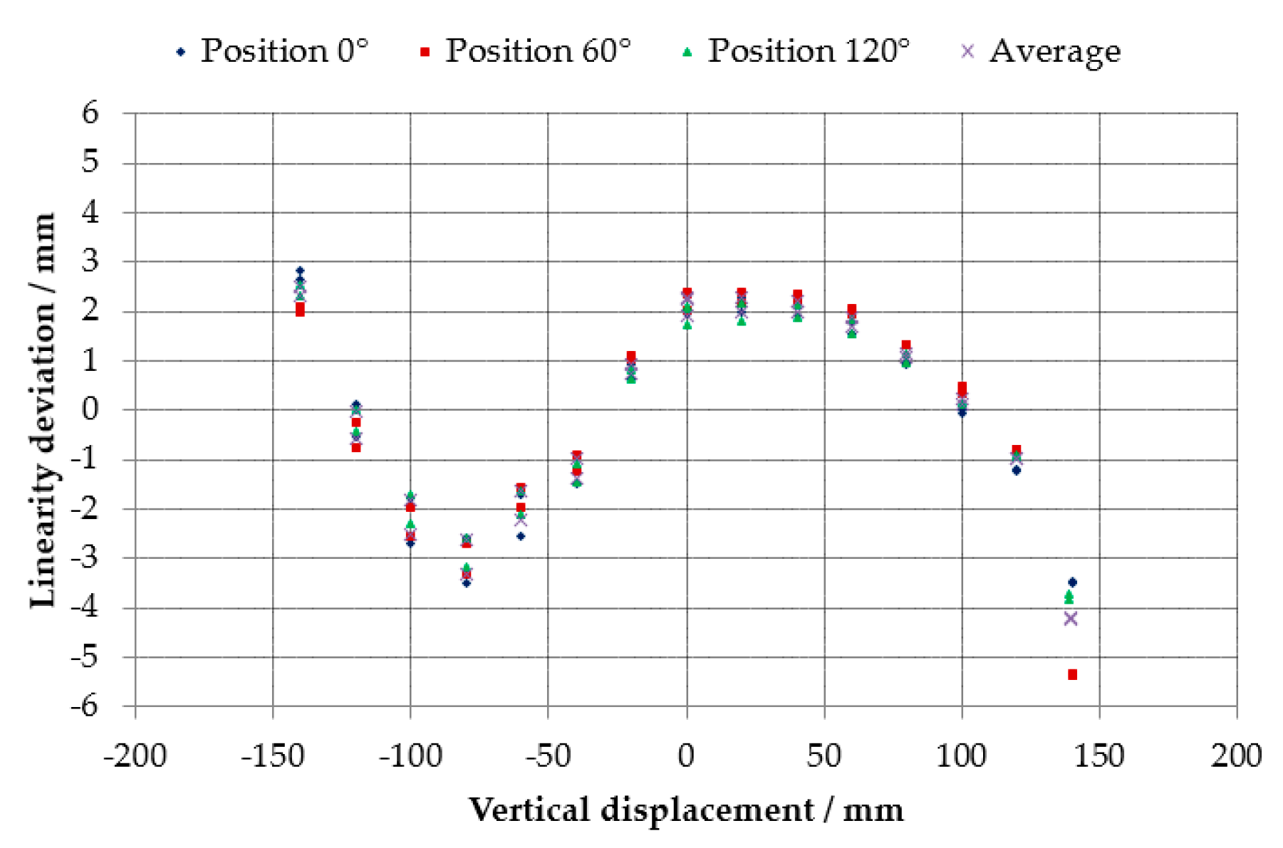
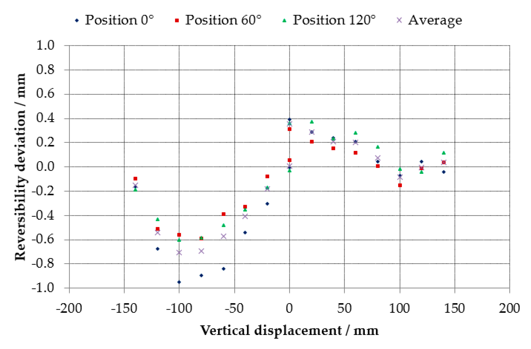
In addition to the water level uncertainty component related with the calibration curve, u(h)_cur (given by Expression 7), the metrological characterization of the conductance transducers allowed to identify the following uncertainty components: linearity, u(h)_lin; dimensional reversibility, u(h)_rev; dimensional stability, u(h)_stb; temperature influence, u(h)_θ,t; and thermal reversibility, u(h)_θ,r. Therefore, the combined measurement uncertainty of the water level obtained by the conductance transducer is given by

$$u\left(h\right)=\sqrt{u{\left(h\right)}_{\mathrm{cur}}^2+u{\left(h\right)}_{\mathrm{lin}}^2+u{\left(h\right)}_{\mathrm{rev}}^2+u{\left(h\right)}_{\mathrm{stb}}^2+u{\left(h\right)}_{\theta ,t}^2+u{\left(h\right)}_{\theta ,r}^2}.$$

(9)

Based on the presented formulation, and taking into account the experimental results shown in Section 4,

Table 6. Measurement uncertainty budget for the ± 140 mm conductance transducer.

Uncertainty Component	Source of Uncertainty	Probability Distribution	Standard Uncertainty	Sensitivity Coefficient	Contribution for Uncertainty	Degrees of Freedom
u(h)lin	Linearity	Uniform	2 mm/√3	1	1.2 mm	50
u(h)rev	Reversibility	Uniform	0.5 mm/√3	1	0.29 mm	50
u(h)rep	Repeatability	Gaussian	0.10 mm	1	0.10 mm	5
u(h)stb	Stability	Gaussian	0.007 mm	1	0.007 mm	29
u(h)θ,t	Temperature influence	Uniform	2 mm/√3	1	1.2 mm	50
u(h)θ,r	Thermal reversibility	Uniform	0.5 mm/√3	1	0.29 mm	50
u(h)cur	Calibration curve	Gaussian	0.72 mm	1	0.72 mm	43
u(m)	Slope parameter	Gaussian	0.13 mm∙V−1	5 V	0.65 mm
u(b)	Intercept parameter	Gaussian	0.78 mm	1	0.78 mm
u(V)	Output voltage	Gaussian	0.0013 V	−29.74 mm∙V−1	0.039 mm	30
u(V)cal	Multimeter calibration	Gaussian	0.00019 V	1	0.00019 V	50
u(V)drf	Drift	Uniform	0.000024 V/√3	1	0.000014 V	50
u(V)res	Resolution	Uniform	0.000005 V/√3	1	0.000003 V	50
u(V)stb	Signal stability (noise)	Gaussian	0.0013 V	1	0.0013 V	29

presents the measurement uncertainty budget, which supported the determination of the instrumental uncertainty of the short-range (±140 mm) conductance transducer, for a nominal output voltage equal to 5 V (DC), and considering a correlation factor of −0.88 between linear parameters of the calibration curve.

Based on the results presented in Table 6, a combined measurement uncertainty of 1.7 mm was obtained for the conductance transducer. The calculated number of effective degrees of freedom is equal to 123, which gives a coverage factor of 2.02, considering a 95% level of confidence. Therefore, the expanded measurement uncertainty of the conductance transducer is equal to 3.5 mm. Additional calculations were performed the voltage measurement interval comprised between 0.5 V and 10 V, for which a maximum value of 3.7 mm for the expanded measurement uncertainty was obtained in the measurement interval limits. This minor increase is justified by the higher measurement uncertainty of the calibration curve in the extreme regions of the measurement interval, as expected.

Table 6 shows the linearity and the temperature influence as the two major uncertainty sources for the instrumental uncertainty of the conductance transducer, followed by the calibration curve. In the case of the linearity, this uncertainty component can be improved considering: (i) a reduction of the measurement interval (if suitable of the maritime reduced-scale model observation); (ii) or the use of a higher order calibration curve (a quadratic curve, for example), instead of a linear calibration curve. The temperature influence contribution to the instrumental uncertainty can be reduced if the conductance transducer is operated under controlled environmental conditions, as it was the case of the linearity, reversibility, and repeatability tests, which supported the determination of the calibration curve.

6. Discussion

The performed study showed that the proposed metrological characterization methods are suitable for the determination of the instrumental measurement uncertainty of conductance transducers used in maritime reduced-scale models, and can be used as a regular laboratorial calibration method, making water level measurements traceable to the SI. In this context, improvements are still possible, namely, the conductance transducer testing only in a wet condition, which should improve the repeatability and the reversibility of the conductance transducers measurements. Special care should also be given to measurements performed in extreme regions of the measurement interval.

The developed instrumental measurement uncertainty evaluation procedure is now available for application in the wide range of LNEC’s conductance transducers. The obtained values can be accounted for in field and computational simulations, therefore, improving the study of the physical phenomena.

Future work will be focused in the metrological study of in situ application of LNEC’s conductance transducers in maritime reduced-scale models, since this study revealed a significant impact of the electrical and environmental influence in the measurement accuracy. Validation of in situ on-the-job verification procedures is a key issue, which will be considered in the near future, namely, the development of measurement standards and methods able to provide in situ traceability transfer.

References

1. Hughes, S.A. Physical Models and Laboratory Techniques in Coastal Engineering; World Scientific Publishing: Singapore, 1993; Volume 7. [Google Scholar]
2. Gerritsen, H.; Stherland, J.; Deigaard, R.; Sumer, B.M.; Fortes, J.; Sierra, J.; Prepernau, U. Guidelines for Composite Modelling of the Interactions between Beaches and Structures; HYDRALAB-III Deliverable JRA1.4; HYDRALAB, EU: København, Denmark, 2009. [Google Scholar]
3. Briggs, M.J. Basics of Physical Modeling in Coastal and Hydraulic Engineering; US Army Engineer Research and Development Center: Vicksburg, MS, USA, 2013. [Google Scholar]
4. Barthel, V.; Funke, E.R. Hybrid modelling as applied to hydrodynamic research and testing. In Recent Advances in Hydraulic Physical Modelling; Martins, R., Ed.; Kluwer Academic Publishers: Berlin, Germany, 1989; Volume 165. [Google Scholar]
5. Kamphuis, J.W. Coastal modeling—A retrospective. In Proceedings of the 6th International Conference on the Application of Physical Modelling in Coastal and Port Engineering and Science—Coastlab16, Ottawa, ON, Canada, 10–13 May 2016. [Google Scholar]
6. Reis, M.T.; Silva, L.G.; Neves, M.G.; Lemos, R.; Capitão, R.; Fortes, J. Physical Modelling as a Fundamental Tool for the Design of Harbors and Maritime Structures; PIANC: Brussels, Belgium, 2015; pp. 135–145. [Google Scholar]
7. Couriel, E.; Nielsen, L.; Jayewardene, I.; McPherson, B. The Need for Physical Models in Coastal Engineering. In Proceedings of the 36th Conference on Coastal Engineering, Baltimore, MD, USA, 30 July–3 August 2018; Lynett, P., Ed.; University of Southern California: Baltimore, MD, USA, 2018. [Google Scholar]
8. Hughes, S.A. Coastal engineering challenges in a changing world. J. Appl. Water Eng. Res. 2014, 2, 72–80. [Google Scholar] [CrossRef]
9. GUM. Guide to the Expression of Uncertainty in Measurement, 1st ed.; ISO—International Organization for Standardization (ISO): Genève, Switzerland, 1993. [Google Scholar]
Figure 1. Conductance transducer developed by LNEC.
Applsci 11 03772 g001
Figure 2. Schematic representation of the experimental setup for the electrical stability test (loaded condition).
Applsci 11 03772 g002
Figure 3. Experimental setup for the linearity, reversibility, and repeatability test of conductance transducers.
Applsci 11 03772 g003
Figure 4. Mechanical connection of the conductance transducer to the testing machine movable cross head in three separated rotations: (a) 0° position; (b) 60° position; (c) 120° position.
Applsci 11 03772 g004
Figure 5. Water reservoir for conductance transducer thermal testing: (a) schematic representation; (b) developed prototype.
Applsci 11 03772 g005
Figure 6. Installation of the instrumented water reservoir inside the climatic chamber.
Applsci 11 03772 g006
Figure 7. Input voltage record for the custom-made power supply in the empty condition.
Applsci 11 03772 g007
Figure 8. Input voltage record for the off-the-shelf power supply in the empty condition.
Applsci 11 03772 g008
Figure 9. Input voltage record related to the loaded condition test with the long-range transducer.
Applsci 11 03772 g009
Figure 10. Output voltage record related to the loaded condition test with the long-range transducer.
Applsci 11 03772 g010
Figure 11. Input voltage record related to the loaded condition test with the short-range transducer.
Applsci 11 03772 g011
Figure 12. Output voltage record related to the loaded condition test with the short-range transducer.
Applsci 11 03772 g012
Figure 13. Relation between the input voltage of the ±400 mm conductance transducer and the applied vertical displacement.
Applsci 11 03772 g013
Figure 14. Relation between the output voltage of the ±400 mm conductance transducer and the applied vertical displacement.
Applsci 11 03772 g014
Figure 15. Linearity deviations of the ±400 mm conductance transducer.
Applsci 11 03772 g015
Figure 16. Reversibility deviations of the ±400 mm conductance transducer.
Applsci 11 03772 g016
Figure 17. Repeatability of the ±400 mm conductance transducer.
Applsci 11 03772 g017
Figure 18. Relation between the input voltage of the ±140 mm conductance transducer and the applied vertical displacement.
Applsci 11 03772 g018
Figure 19. Relation between the output voltage of the ±140 mm conductance transducer and the applied vertical displacement.
Applsci 11 03772 g019
Figure 20. Linearity deviations of the ±140 mm conductance transducer.
Applsci 11 03772 g020
Figure 21. Reversibility deviations of the ±140 mm conductance transducer.
Applsci 11 03772 g021
Figure 22. Repeatability of the ±140 mm conductance transducer.
Applsci 11 03772 g022
Figure 23. Water and air temperature records during the thermal test.
Applsci 11 03772 g023
Figure 24. Input voltage of the conductance transducer during the thermal test.
Applsci 11 03772 g024
Figure 25. Output voltage of the conductance sensor during the thermal test.
Applsci 11 03772 g025
Figure 26. Relative variation of the water level in the conductance transducer during the thermal test.
Applsci 11 03772 g026