Article

Seepage Mechanism of Tight Sandstone Reservoir Based on Digital Core Simulation Method

1
The State Key Laboratory of Management and Control for Complex Systems & the Beijing Engineering Research Center of Intelligent Systems and Technology, Institute of Automation, Chinese Academy of Sciences, Beijing 100190, China
2
Institute of Information Engineering, Chinese Academy of Sciences, Beijing 100190, China
3
Cloud Computing Center, Chinese Academy of Sciences, Dongguan 610225, China
4
Qingdao Academy of Intelligent Industries, Chinese Academy of Sciences, Qingdao 266114, China
5
School of Artificial Intelligence, University of Chinese Academy of Sciences, Beijing 100049, China
*
Authors to whom correspondence should be addressed.
Appl. Sci. 2021, 11(9), 3741; https://doi.org/10.3390/app11093741
Submission received: 17 February 2021 / Revised: 26 March 2021 / Accepted: 16 April 2021 / Published: 21 April 2021
(This article belongs to the Special Issue Artificial Intelligence and Emerging Technologies)

Abstract

:
Recently, tight sandstone oil has played an increasingly important role in the energy strategies of countries around the world. However, the understanding of a microscopic mechanism is still not clear enough, which has been affecting the improvement of the recovery of tight sandstone oil. In this article, a digital core model was established to simulate the pore network of a physical core with CT scan and difference equations were verified by Fourier counting. Then, a combination of orthogonal tests and cubic digital cores was used to experimentally investigate various parameters including pressure, length, permeability, viscosity, and time. By combining the physical experiments with the digital core methods, it can be observed that the state of the micro-crack affects the conductivity of the core, which may be the decisive reason for changing the pressure gradient. The orthogonal test showed that the sensitivity of the parameters was pressure, length, permeability, time, and viscosity in order. The results of the numerical simulations showed that this method can reveal the seepage mechanism of a tight sandstone reservoir, greatly shortening the experimental time and improving flexibility.

1. Introduction

Reservoirs with a permeability of less than 0.1 mD are generally referred to as tight sandstone reservoirs [1]. From 2000 to 2017, production of tight sandstone oil has increased. In 2019, accounting for 53% of a total crude oil product in the United States [2]. The multi-stage and multi-cluster fracturing technologies in horizontal wells have become the main means while developing tight sandstone oil [3]. When fractured, enormous micro-cracks form in the reservoir around the bottom of the hole, causing the formation of small pieces and improving the conductivity of the reservoir.
At present, there are many macroscopic studies on the seepage problem of a reservoir matrix-fracture dual system, but research studies on the law of matrix failure at a microscopic level are rare [4,5]. Moreover, the study of the seepage law of the matrix now is of great importance for developing tight sandstone oil reservoirs effectively. Liu et al. suggested that distribution of tight sandstones could be observed by Octamethylcyclotetrasiloxane [6]. Several researchers noted that a microscopic mechanism in seepage could be observed by the combination of an indoor experiment and a lithography physical model [2,7]. Taken together, many researchers have done a lot of work and achieved remarkable achievement [3,4,8,9]. However, due to strict experimental conditions and a preparation cycle, many of the above experiments cannot be repeated, or have a high cost.
In this paper, a more convenient method combining the physical experiment with a digital core is designed to reveal seepage mechanism at a microscopic level and greatly shorten the experimental time. First, the digital core for the simulation calculation is established for the subsequent simulated annealing algorithm to build the matrix block simulation. Then, the system simulation results of the core are compared with the indoor experimental results to verify the accuracy of the simulation model. The simulation shows that the opening and closing state of the micro-crack affects the conductivity of the core, which may be the reason for the starting pressure gradient [10]. The pros and cons of methods such as Gaussian field method [11], simulated the annealing method [12], and the Markov chain-Monte Carlo method [13] are discussed. Finally, the pore network model established by a simulated annealing algorithm is used to construct three-dimensional matrix cubes with different parameters. The orthogonal test method [14] was used to combine different levels of various parameters. The factors affecting the degree of exhaustion were analyzed and finally sorted to guide production practices.
The rest of this paper is listed as follows. Section 1 introduces the digital core modeling methods. Section 2 proposes the different equations for digital cores. Section 3 presents and analyzes the stability of different equations. Finally, the results and discussion are drawn in Section 4.

2. Modeling of the Digital Core

Indoor experimental analysis methods can determine the physical properties of cores by using the fixed instruments and methods [2], which we use to analyze and optimize the elliptical flow around the well bottom shown in Figure 1. The fixed instruments mainly include pumps and core holders. When using this method individually, the cycle and cost will be tremendous. Additionally, it may cost several days or even longer to retrieve complete data of recovery versus time. However, this method needs a lot of time and cost. Scanning electron microscopy imaging by CT is done to excite a beam of electrons to the surface of the sample, under the region where the electrons in the inner layer are bombarded by foreign electrons [15,16]. The characteristic X-ray spectrum with the mineral component information is received by the optical signal receiver. Thus, a point-by-point scan of the core surface provides an image of the mineral distribution on the surface of the core sample [13]. This type of simulation technology can estimate core parameters using minimal cost in a very short time [17]. Since it can model the pore structure inside the core, the microscopic seepage mechanism inside the core can be visually revealed in the simulation process.
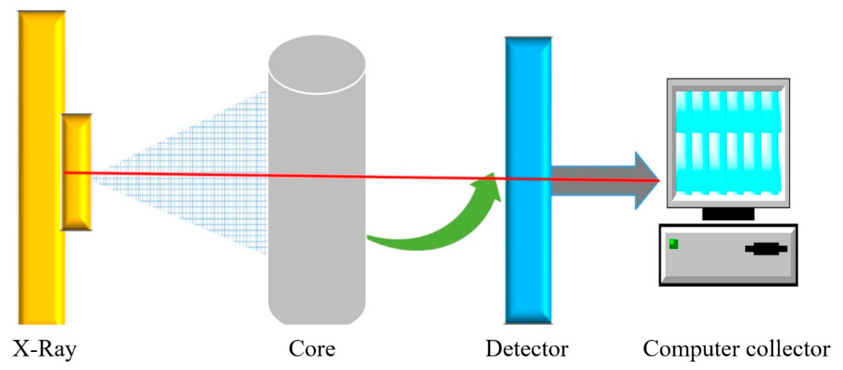
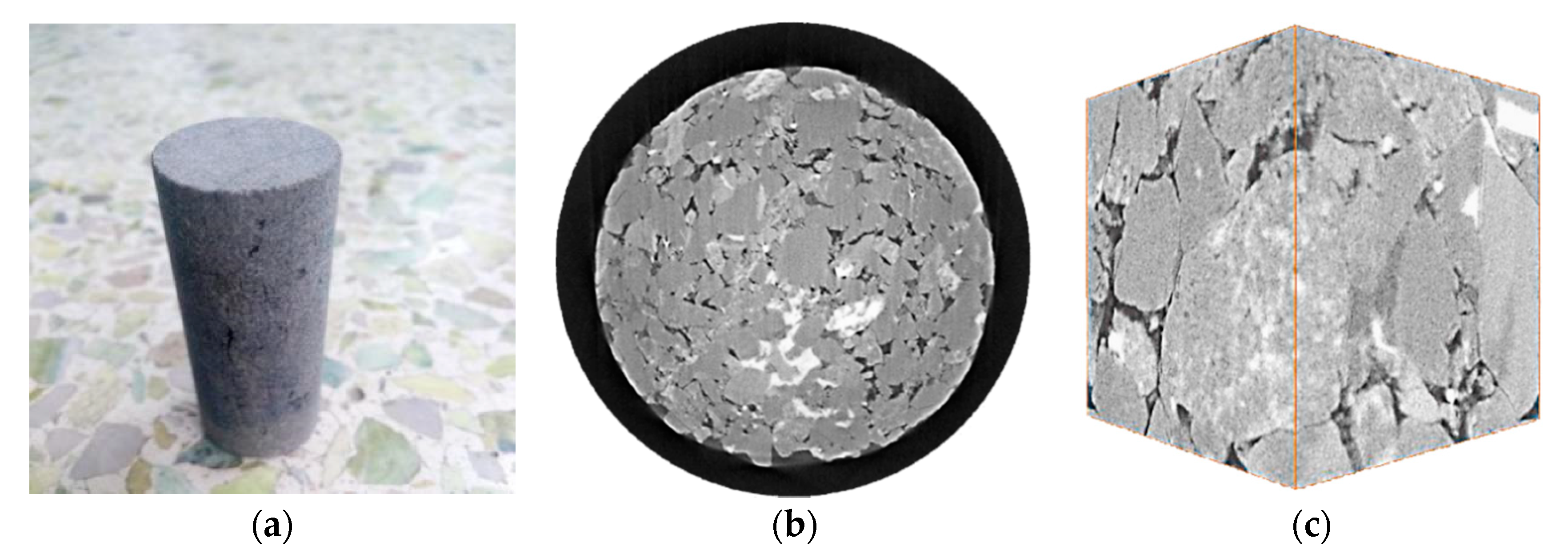
The method used in rock mass scanning is to accurately control the parameters of the CT testing machine through a computer shown in Figure 2. The X-ray generator (Zeiss) then emits X-rays that penetrate the sample fixed and to be rotated on the sample holder. The other end is an X-ray detector and the data acquisition system of the CT machine collects the data acquired by the detector [18]. Finally, the holder was rotated at a certain speed and was re-recorded. The cumulative rotation is 360°. The CT scanning and modeling process are shown in Figure 3.
The plunger-shaped core is placed into the CT scanner to obtain a CT scan sectional view. By modeling the scanned images of different sections and angles, a 3D pore network model of the plug core is obtained as shown in Figure 4.

3. Difference Equations for Digital Cores

For the core numerical model, the difference equations for pressure propagation need to be specified [19]. It is assumed that the nth time step physical quantity P of the problem is known and the n+1 time step P value is to be sought. Choose any time and space point (i, j, k, n + 1). P(x, y, z, t) is substituted for the second-order difference quotient of (x, y, z) and the backward difference quotient of t at any point (x, y, z, t) to obtain difference equations at any point (i, j, k, n + 1).
a P i + 1 , j , k n + 1 + c P i 1 , j , k n + 1 + a P i , j + 1 , k n + 1 + c P i , j 1 , k n + 1 + a P i , j , k + 1 n + 1 + c P i , j , k 1 n + 1 + b P i , j , k n + 1 = P i , j , k n
Among them:
a = η Δ t ( G C L h 1 h 2 ) ,   b = 6 η Δ t h 2 3 G C L η Δ t h + 1 ,   c = η Δ t h 2 .
For the symbols appearing above, the physical meaning of each symbol is shown in Table 1.

4. Stability Analysis of Difference Equations

Using the Fourier analysis [20,21] method, let the error be ε and get the error equation as:
1 h 2 ( ε i + 1 n + 1 2 ε i n + 1 + ε i 1 n + 1 + ε j + 1 n + 1 2 ε j n + 1 + ε j 1 n + 1 + ε k + 1 n + 1 2 ε k n + 1 + ε k 1 n + 1 ) G C L h ( ε i + 1 n + 1 ε i n + 1 + ε j + 1 n + 1 ε j n + 1 + ε k + 1 n + 1 ε k n + 1 ) = 1 η ( ε n + 1 ε n + 1 Δ t )
According to the principle of Fourier series [19,20,21], the error term is written as a simple harmonic (complex) form.
ε j n = A n e i k x j
The growth factor A was obtained as follows.
A = 1 1 + 6 η Δ t h 2 ( 1 cos k h ) + η Δ t G C L h ( 3 cos k h + 3 i sin k h 3 )
It is known that |A| ≤ 1. Therefore, the difference equation is unconditionally stable and the numerical model can be directly used to solve the equations.

4.1. Parameter Selection

Dividing the indoor experiments into four groups, the downstream pressures were 0 MPa, 10 MPa, 20 MPa, and 30 MPa, respectively, and the initial value of the upstream pressure remained unchanged at 43 MPa. By comparing the output cumulative yield and pressure distribution at different outlet pressures at the same time, the difference between the digital core model and the physical experiment can be verified, thereby, verifying the validity of the numerical model.
The parameters of the example mentioned next are shown in Table 2.

4.2. D Matrix Block Modeling

The pore network model in Figure 4c is modeled by a scanned image. In order to study the 3-dimensional space rather than the one-dimensional seepage law, it is necessary to re-establish the dense matrix model with a fast pore network in 3D space. Extending the dimension makes it satisfy the statistical structure of the pore structure of the original numerical model. Current mainstream statistical modeling methods include Gaussian field method simulated annealing and the Markov chain-Monte Carlo method. Compared with the Gaussian field method, the simulated annealing method can take more rock information into account, making the model closer to the real core [22,23]. Compared with the Markov-Monte Carlo method, the complexity of simulated annealing is lower.
We only regard the core model as a two-phase system of rock skeletons and pores. Since the space where the fluid is the pore, the calculation of each characteristic function value focuses on the pore space. The modeling objective function is composed of the autocorrelation function of the reconstruction system and the reference system. The objective function of the system at a certain time can be defined as follows.
E = i α i [ S r ( r i ) S ( r i ) ] 2 + i β i [ L r ( r i ) L ( r i ) ] 2
where α i , β i are the weight value of the different constraint functions and E is the total energy of the system.
S ( r ) represents the probability that two points of any distance r in the system are simultaneously pore phases [15]. It has the property S 2 j ( 0 ) = φ j , and j represents the jth phase.
L ( r ) is the connectivity function of the pores and r is the distance between the two points. For a one-way system with a porosity of φ , L ( 0 ) = φ .
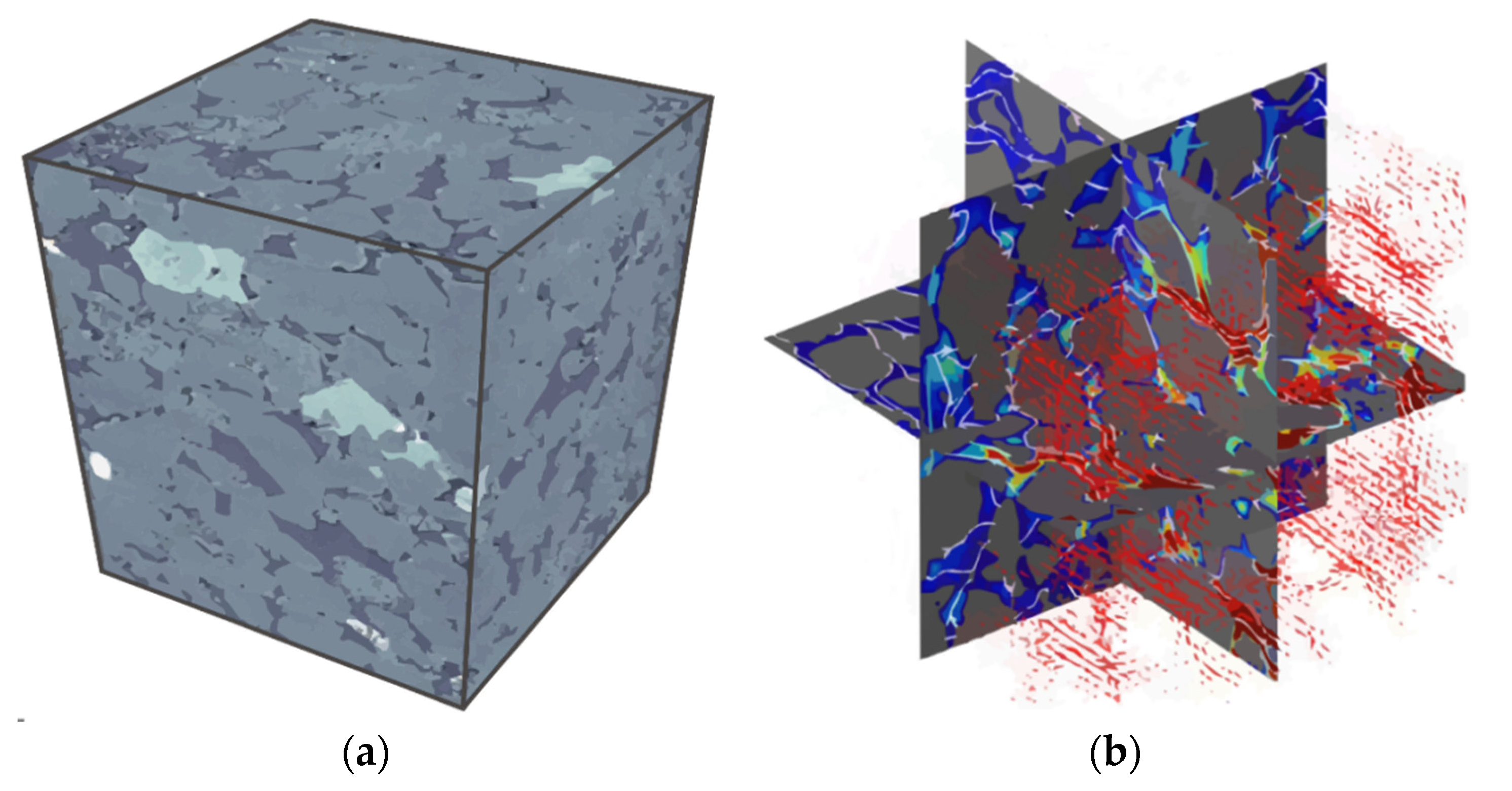
The digital core modeling steps are as follows: (1) Binarize the actual core CT image or electron microscope scan image, collect model statistics φ , S ( r ) , L ( r ) . (2) Randomly generate a three-dimensional digital core with a porosity of 0.3 and calculate the initial model objective function E to enter the optimization process. (3) Take a hole point and a skeleton point arbitrarily and interchange their positions to generate a new system, and then calculate the objective function E. (4) The new system is determined by the Metropolis criterion if it is good enough to replace the old system in order (5) to decide whether to terminate the cycle according to the inner and outer loop termination condition. (6) Finally, output the digital core simulation results and end the process [16,24]. The modeling results are shown in Figure 5.

4.3. Orthogonal Test Analysis

After verifying the validity of the numerical model, the scope of theoretical research can be extended to a three-dimensional space. We study the sensitivities of different factors regarding the efficiency of a dense matrix failure. Figure 6 is an example of a pressure field simulation of a depletion process.
Moreover, theoretical studies were carried out using orthogonal experiments. A total of 16 orthogonal experiments were performed and a total of 5 factors and 4 levels (0 MPa, 10 MPa, 20 MPa, and 30 MPa) were selected with results of the selection being shown in Table 3 below. In addition, the boundary pressure is set to 0, while the remaining settings are the same with Table 2.

4.4. Results and Discussion

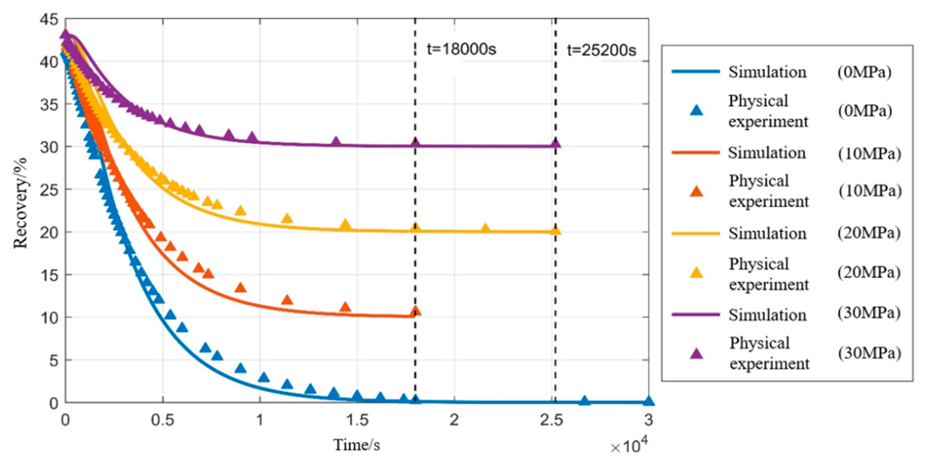
By comparing the simulated value with the physical one, mutual verification of digital and physical models can be performed. In the comparison, the upstream pressures under four gradients are taken. They are 0 MPa, 10 MPa, 20 MPa, and 30 MPa, respectively. The time to get the last data point is 30,000 s, 18,000 s, 25,200 s, and 25,200 s, so the numerical simulation is the same as the measured time in the laboratory. A comparison of the recovery ratio of the theoretical and measured curves under upstream pressure was made and shown in Figure 7.
From the comparison of Figure 7, it can be observed that the established numerical model is very close to the actual core physical properties. The final exhaustion yields are basically coincidental, which indicates the effectiveness of digital core technology.
(1) The theoretical and measured recovery factors have a large error in the early stage of exhaustion mining. However, as the mining time increases, the theoretical model and the measured recovery data begin to approach. At the end of exhaustion, the theoretical and measured results are basically coincident. The reason for this is that the digital core ignores interfacial tension between gas and oil, thus, resulting in a different flow state at the end of a digital one compared to a physical one.
(2) The relative error between the numerical model and physical experiment is not large, but the four sets of contrast curves show the high pressure of the previous theoretical model. The reason is that, in the early stage of exhaustion mining, the pressure drop of the theoretical model has not yet propagated upstream. Therefore, the upstream pressure remains unchanged during the next period of mining start.
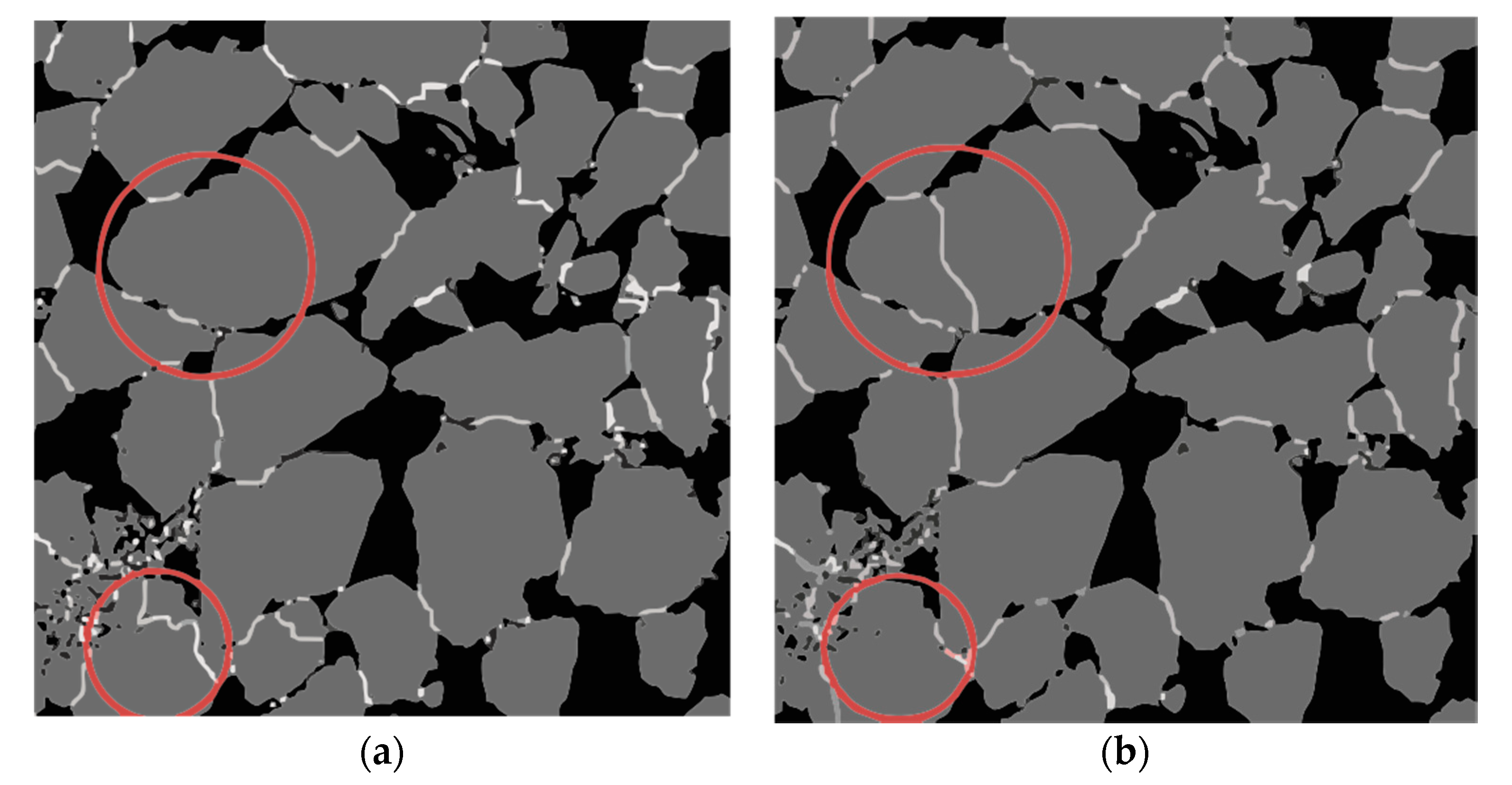
Additionally, during the numerical simulation, an interesting phenomenon in which some cracks have both open and closed states is observed. This phenomenon gives a microscopic interpretation clearly of the starting pressure gradient of a tight reservoir. As shown in Figure 8a, a plan view of the model at a pressure differential of 10 MPa (b) corresponding to a plan view of the model at a pressure of 40 MPa. It can be observed that the micro-cracks within the marked range are in a closed state when the pressure difference of failure is 10 MPa. However, it is turned on under the depletion pressure difference of 40 MPa. It explains, at a microscopic level, why there is a starting pressure gradient in a tight sandstone reservoir in the case of a low pressure difference.
Furthermore, 16 calculations of the orthogonal test were performed according to the selected five factors and four levels, and the simulation results are shown in Table 4.
The calculation results on the orthogonal test were analyzed by considering the absolute deviation of each parameter, and the results are listed in Table 5.
It can be seen from the results in Table 5 that the change of pressure has the largest influence on tight oil recovery and the change of viscosity has the smallest one. Furthermore, the parameters in order of sensibility are pressure, length, permeability, time, and viscosity.

5. Conclusions

The research method, which combines a physical experiment with digital core methods, can greatly shorten the experimental period. In addition, after verifying the accuracy of the 3D digital core, the scale shape and production system of the research object can be arbitrarily changed. By this way, the approach greatly increases the flexibility of the research and all of them complete the experiment in a short period. This promising research method is applied to the matrix failure process of tight reservoirs, which can reveal the seepage mechanism of a tight sandstone reservoir as follows.
(1) The macroscopic starting pressure gradient is embodied in the microscopic pore structure. Under the lower exhaustion pressure difference, part of the micro-crack is in the closed state. When the pressure rises, the crack reopens, thereby, increasing the conductivity of the reservoir.
(2) Considering the time scale, the core recovery is analyzed by the orthogonal test. Then the factors, in order of importance, are pressure, length, permeability, time, and viscosity.

Author Contributions

Conceptualization, H.W.; Formal analysis, X.D.; Investigation, Z.S.; Methodology, X.D.; Project administration, G.X.; Writing—original draft, Y.X.; Writing—review & editing, Y.W. All authors have read and agreed to the published version of the manuscript.

Funding

The work was supported, in part, by the National Natural Science Foundation of China under Grants U19B2029, 61872365, 61773382, 61773381, and U1909204, CAS Key Technology Talent Program (Zhen Shen), and Hunan Province Science and Technology Program under Grants 2018GK1040.

Institutional Review Board Statement

Not applicable.

Informed Consent Statement

Not applicable.

Data Availability Statement

All data generated or analyzed during this study are included in this manuscript.

Conflicts of Interest

The authors declare no conflict of interest

References

  1. Du, S.; Pang, S.; Shi, Y. Quantitative characterization on the microscopic pore heterogeneity of tight oil sandstone reservoir by considering both the resolution and representativeness. J. Pet. Sci. Eng. 2018, 169, 388–392. [Google Scholar] [CrossRef] [Green Version]
  2. Zhang, Y.; Zeng, J.; Dai, Z.; Viswanathan, H.; Xiao, T.; Ma, Y.; Feng, X. Experimental investigation on oil migration and accumulation in tight sandstones. J. Pet. Sci. Eng. 2018, 160, 267–275. [Google Scholar] [CrossRef]
  3. Hu, S.; Zhou, C.; Li, X.; Li, C.; Zhang, S. A tight sandstone trapezoidal pore oil saturation model. Pet. Explor. Dev. 2017, 44, 876–886. [Google Scholar] [CrossRef]
  4. Li, J.; Li, X.R.; Song, M.S.; Liu, H.M.; Feng, Y.C.; Liu, C. Investigating microscopic seepage characteristics and fracture effectiveness of tight sandstones: A digital core approach. Pet. Sci. Vol. 2021, 18, 173–182. [Google Scholar] [CrossRef]
  5. Lai, J.; Wang, G.; Chen, J.; Wang, S.; Zhou, Z.; Fan, X. Origin and Distribution of Carbonate Cement in Tight Sandstones: The Upper Triassic Yanchang Formation Chang 8 Oil Layer in West Ordos Basin, China. Geofluids 2017, 2017, 8681753. [Google Scholar] [CrossRef] [Green Version]
  6. Liu, B.; Yao, S.; Hu, W.; Cao, J. Applying octamethylcyclotetrasiloxane as a probe liquid for characterizing the pore size distribution of oil-bearing tight sandstones by nuclear magnetic resonance cryoporometry. Mar. Pet. Geol. 2017, 88, 814–825. [Google Scholar] [CrossRef]
  7. Xi, K.; Cao, Y.; Liu, K.; Zhu, R. Factors influencing oil saturation and exploration fairways in the lower cretaceous Quantou Formation tight sandstones, Southern Songliao Basin, China. Energy Explor. Exploit. 2018, 36, 1061–1085. [Google Scholar] [CrossRef] [Green Version]
  8. Yilmaz, M.; Tugrul, A. The effects of different sandstone aggregates on concrete strength. Constr. Build. Mater. 2012, 35, 294–303. [Google Scholar] [CrossRef]
  9. Petrounias, P.; Giannakopoulou, P.P.; Rogkala, A.; Kalpogiannaki, M.; Koutsovitis, P.; Damoulianou, M.E.; Koukouzas, N. Petrographic Characteristics of Sandstones as a Basis to Evaluate Their Suitability in Construction and Energy Storage Applications. A Case Study from Klepa Nafpaktias (Central Western Greece). Energies 2020, 13, 119. [Google Scholar] [CrossRef] [Green Version]
  10. Bessa, M.A.; Bostanabad, R.; Liu, Z.; Hu, A.; Apley, D.W.; Brinson, C.; Chen, W.; Liu, W.K. A framework for data-driven analysis of materials under uncertainty: Countering the curse of dimensionality. Comput. Methods Appl. Mech. Eng. 2017, 320, 633–667. [Google Scholar] [CrossRef]
  11. Bodla, K.K.; Garimella, S.V.; Murthy, J.Y. 3D reconstruction and design of porous media from thin sections. Int. J. Heat Mass Transf. 2014, 73, 250–264. [Google Scholar] [CrossRef] [Green Version]
  12. Ferreira, K.M.; de Queiroz, T.A. Two effective simulated annealing algorithms for the Location-Routing Problem. Appl. Soft Comput. 2018, 70, 389–422. [Google Scholar] [CrossRef]
  13. Bostanabad, R.; Bui, A.T.; Xie, W.; Apley, D.W.; Chen, W. Stochastic microstructure characterization and reconstruction via supervised learning. Acta Mater. 2016, 103, 89–102. [Google Scholar] [CrossRef] [Green Version]
  14. Feng, J.; Teng, Q.; He, X.; Qing, L.; Li, Y. Reconstruction of three-dimensional heterogeneous media from a single two-dimensional section via co-occurrence correlation function. Comput. Mater. Sci. 2018, 144, 181–192. [Google Scholar] [CrossRef]
  15. Izadi, H.; Baniassadi, M.; Hasanabadi, A.; Mehrgini, B.; Memarian, H.; Soltanian-Zadeh, H.; Abriniac, K. Application of full set of two point correlation functions from a pair of 2D cut sections for 3D porous media reconstruction. J. Pet. Sci. Eng. 2017, 149, 789–800. [Google Scholar] [CrossRef]
  16. Xu, H.; Dikin, D.A.; Burkhart, C.; Chen, W. Descriptor-based methodology for statistical characterization and 3D reconstruction of microstructural materials. Comput. Mater. Sci. 2014, 85, 206–216. [Google Scholar] [CrossRef]
  17. Hajizadeh, A.; Safekordi, A.; Farhadpour, F.A. A multiple-point statistics algorithm for 3D pore space reconstruction from 2D images. Adv. Water Resour. 2011, 34, 1256–1267. [Google Scholar] [CrossRef]
  18. Hasanabadi, A.; Baniassadi, M.; Abrinia, K.; Safdari, M.; Garmestani, H. 3D microstructural reconstruction of heterogeneous materials from 2D cross sections: A modified phase-recovery algorithm. Comput. Mater. Sci. 2016, 111, 107–115. [Google Scholar] [CrossRef]
  19. Mekki, A.; Ali, M.M. Numerical simulation of Kadomtsev–Petviashvili–Benjamin–Bona–Mahony equations using finite difference method. Appl. Math. Comput. 2013, 219, 11214–11222. [Google Scholar] [CrossRef]
  20. Song, G.; Li, Y.; Wang, W.; Jiang, K.; Shi, Z.; Yao, S. Investigation on the mechanical properties and mechanical stabilities of pipewall hydrate deposition by modelling and numerical simulation. Chem. Eng. Sci. 2018, 192, 477–487. [Google Scholar] [CrossRef]
  21. Tomé, M.F.; de Araujo, M.S.B.; Alves, M.A.; Pinho, F.T. Numerical simulation of viscoelastic flows using integral constitutive equations: A finite difference approach. J. Comput. Phys. 2008, 227, 4207–4243. [Google Scholar] [CrossRef]
  22. Okabe, H.; Blunt, M.J. Pore space reconstruction using multiple-point statistics. J. Pet. Sci. Eng. 2005, 46, 121–137. [Google Scholar] [CrossRef]
  23. Zhou, X.P.; Xiao, N. 3D Numerical Reconstruction of Porous Sandstone Using Improved Simulated Annealing Algorithms. Rock Mech. Rock Eng. 2018, 51, 2135–2151. [Google Scholar] [CrossRef]
  24. Saxena, N.; Mavko, G.; Hofmann, R.; Srisutthiyakorn, N. Estimating permeability from thin sections without reconstruction: Digital rock study of 3D properties from 2D images. Comput. Geosci. 2017, 102, 79–99. [Google Scholar] [CrossRef] [Green Version]
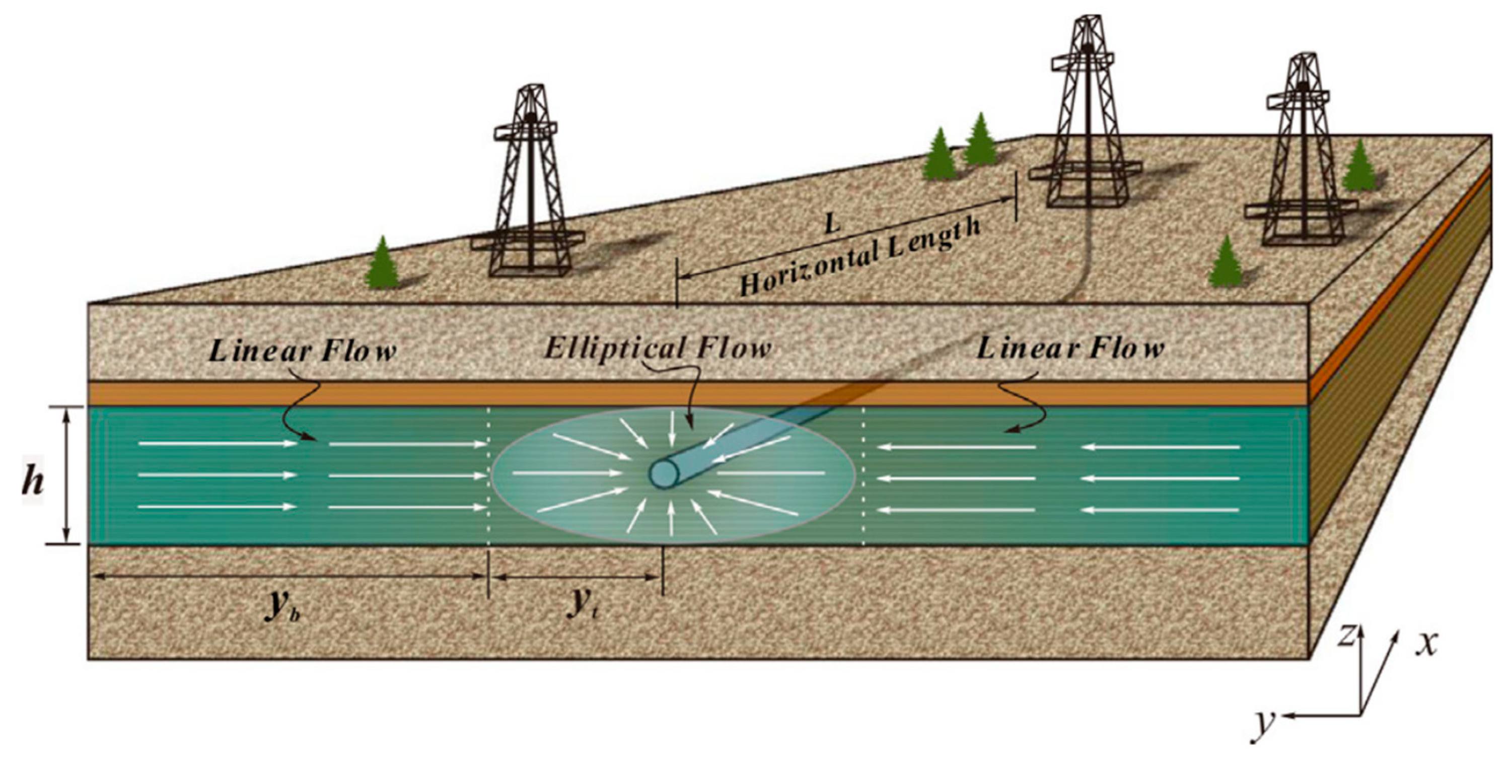
Figure 1. Horizontal well schematic.
Applsci 11 03741 g001
Figure 2. CT scanning device schematic.
Applsci 11 03741 g002
Figure 3. Digital core scanning and modeling images. (a) Plunger core, (b) cross-sectional view by CT, and (c) core numerical model.
Applsci 11 03741 g003
Figure 4. Pore network model. (a) Skeleton model, (b) skeleton and pore, and (c) sectional view of the pore.
Applsci 11 03741 g004
Figure 5. Dense matrix pore network model. (a) Matrix block generated by the algorithm, and (b) pore network inside the matrix block.
Applsci 11 03741 g005
Figure 6. Example of pressure field simulation in a depletion process. (a) Pressure distribution (3 days), and (b) pressure distribution (6 days).
Applsci 11 03741 g006
Figure 7. Comparison of numerical simulation and physical experiment under different upstream pressures.
Applsci 11 03741 g007
Figure 8. Micro-crack state under different pressures. (a) Low pressure, and (b) high pressure.
Applsci 11 03741 g008
Table 1. Symbol convention.
SymbolMeaningSymbolMeaning
vSeepage velocity (cm/d)Cl-Fluid compression factor (MPa−1)
ρDensity of oil (underground) (g/cm3)kMatrix permeability (10−3 μm2)
ρ aDensity of oil (g/cm3)PwDownstream crack pressure (MPa)
LCore length (m)PiOriginal formation pressure (MPa)
CtComprehensive compression factor (MPa−1) u o Crude oil viscosity (mPa · s)
Cf-Rock compression factor (MPa−1) η Pressure coefficient
φ Formation porosityGStarting pressure gradient (MPa/m)
Table 2. Example parameters and values.
ParameterValueParameterValue
Core length (cm)6.77Matrix pressure (Mpa)43
Downstream pressure (Mpa)0–30Matrix permeability (mD)0.075
Crude oil viscosity (mPa·s)1.8Comprehensive compression
factor (MPa−1)
3.6 × 10⁻⁴
Liquid compression factor
(MPa−1)
3 × 10⁻³Starting pressure gradient
(MPa/cm)
3.15 × 10⁻²
Table 3. Influencing factors and level selection table.
FactorPressure (MPa)Viscosity (mPa·s)Permeability (mD)Length (m)Time (h)
Lwvel
1100.60.0753.252.5
2201.20.156.55
3301.80.2259.757.5
4402.40.31310
Table 4. Orthogonal test calculation results.
FactorPressure
(MPa)
Viscosity
(mPa·s)
Permeability
(mD)
Length
(cm)
Time
(h)
Recovery
(%)
Order
1100.60.0753.252.53.27
2101.20.156.553.29
3101.80.2259.757.53.13
4102.40.313102.87
5200.60.159.75106.06
6201.20.075137.53.79
7201.80.33.25515.54
8202.40.2256.52.55.39
9300.60.2251359.96
10301.20.39.752.59.96
11301.80.0756.5109.03
12302.40.153.257.515.51
13400.60.36.57.513.16
14401.20.2253.251012.99
15401.80.15132.59.29
16402.40.0759.7558.64
Table 5. Results of the range method analysis.
FactorPressure (MPa)Viscosity (mPa·s)Permeability (mD)Length (cm)Time (h)
Level
13.148.11256.182511.82756.9775
27.6957.50758.53757.71759.3575
311.1159.24757.86756.94758.8975
411.028.102510.38256.47757.7375
Difference7.9751.1354.25.352.38
Publisher’s Note: MDPI stays neutral with regard to jurisdictional claims in published maps and institutional affiliations.