Article

Unsupervised Cell Segmentation and Labelling in Neural Tissue Images

by
Sara Iglesias-Rey
1,2,*,
Felipe Antunes-Santos
1,2,3,
Cathleen Hagemann
4,5,
David Gómez-Cabrero
2,6,
Humberto Bustince
1,2,
Rickie Patani
4,7,
Andrea Serio
4,5,
Bernard De Baets
3 and
Carlos Lopez-Molina
1,2,3
1
Department of Estadistica, Informatica y Matematicas, Universidad Publica de Navarra, 31006 Pamplona, Spain
2
NavarraBiomed, Complejo Hospitalario de Navarra, 31008 Pamplona, Spain
3
KERMIT, Department of Data Analysis and Mathematical Modelling, Ghent University, 9000 Ghent, Belgium
4
The Francis Crick Institute, 1 Midland Road, London NW1 1AT, UK
5
Centre for Craniofacial & Regenerative Biology, King’s College London, London WC2R 2LS, UK
6
Biological and Environmental Sciences and Engineering Division, King Abdullah University of Science and Technology (KAUST), Thuwal 23955, Saudi Arabia
7
Department of Neuromuscular Diseases, UCL Queen Square Institute of Neurology, Queen Square, London WC1N 3BG, UK
*
Author to whom correspondence should be addressed.
Appl. Sci. 2021, 11(9), 3733; https://doi.org/10.3390/app11093733
Submission received: 14 March 2021 / Revised: 12 April 2021 / Accepted: 18 April 2021 / Published: 21 April 2021
(This article belongs to the Special Issue Medical Artificial Intelligence)

Abstract

:
Neurodegenerative diseases are a group of largely incurable disorders characterised by the progressive loss of neurons and for which often the molecular mechanisms are poorly understood. To bridge this gap, researchers employ a range of techniques. A very prominent and useful technique adopted across many different fields is imaging and the analysis of histopathological and fluorescent label tissue samples. Although image acquisition has been efficiently automated recently, automated analysis still presents a bottleneck. Although various methods have been developed to automate this task, they tend to make use of single-purpose machine learning models that require extensive training, imposing a significant workload on the experts and introducing variability in the analysis. Moreover, these methods are impractical to audit and adapt, as their internal parameters are difficult to interpret and change. Here, we present a novel unsupervised automated schema for object segmentation of images, exemplified on a dataset of tissue images. Our schema does not require training data, can be fully audited and is based on a series of understandable biological decisions. In order to evaluate and validate our schema, we compared it with a state-of-the-art automated segmentation method for post-mortem tissues of ALS patients.

1. Introduction

Neurodegeneration is a broad concept that generally refers to any pathology that features the loss of neuronal populations [1]. Although different Neurodegenerative Diseases (NDs) are caused by various molecular events and present distinct clinical features, they often share a significant number of pathological hallmarks. Therefore, research strategies and tools used to study NDs are often similar. Relevant examples of NDs are Alzheimer’s disease [2], Amyotrophic Lateral Sclerosis (ALS) [3] or Parkinson’s disease [4], where different neuronal populations are selectively affected, but present shared molecular features that can be investigated using the same tools. Over the past few years, with the increase in life expectancy, the relevance of NDs has increased significantly [5], boosted by the fact that the vast majority of these pathologies are incurable and with limited therapeutic options.
Research on NDs involves different strategies and disciplines, and as a result, it has evolved into a broad interdisciplinary field focused on efforts to understand, prevent and alleviate the molecular effects of neurodegeneration. Therefore, a significant part of this effort is devoted to understanding the molecular mechanisms of neurodegeneration at the single-cell level, both in the form of observational experiments to identify specific molecular phenotypes (e.g., imaging studies on affected vs. unaffected neurons to assess mislocalisation of key proteins) and by follow-up interventional hypothesis-testing studies (e.g., treatment with potential therapeutic molecules to alter the observed disease phenotype). The vast majority of these studies are based on microscopy observation of the neuronal population affected, either in vitro within cell culture models or from ex vivo or post-mortem samples.
As microscopy technology advances, widespread adoptions of high-content screening [6,7] and imaging with automated microscopy [8] have revolutionised the way of using imaging-based analysis, especially for neurodegeneration molecular phenotyping either in vitro [9,10] or ex vivo [11,12]. As a result, researchers have increased throughput and analytical power in their studies, as the imaging systems can automatically acquire thousands of images. Additionally, the possibility of increasing the availability and size of imaging datasets has been instrumental also for molecular pathology laboratories dealing directly with biopsies from patients or post-mortem samples. However, as an associated outcome, the bottleneck has been shifted towards analysing these large datasets where information needs to be gathered, potentially at a single-cell level, benefiting the in-depth analysis of heterogeneous samples.
In many laboratories, the analysis of these datasets has as its main prerequisite the necessity of correctly identifying the neurons (or other cell types). Furthermore, it is often relevant to further segment the cells into their constituent parts (e.g., nucleus, axons, cell bodies, etc.) to perform more detailed molecular analyses, like protein localisation [11]. Moreover, other experiments might require the extraction of more precise data from the images at a population level (for example, the neural network) or even viability or mitosis rates over a certain period of time [13].
In the data extraction context, identifying target cells and the segmentation of morphological features are some of the most crucial phases and are often performed either manually or in a semi-supervised way, leading to an increase in human workload. Moreover, this phase can be seen as both a goal itself or as a pre-processing step in image-associated molecular studies. The literature contains a vast number of methods that are fully or partially aimed at object segmentation in ND-related imaging [14,15,16]. The development of reliable intelligent image processing techniques for neuronal analysis is far from trivial and is, often, heavily dependent on the image characteristics, which can be altered by factors including the biological configuration of the populations or the physical setup in which the images are acquired. However, the main problem in designing these techniques lies in the modelling of the understanding of human operators, as it is critical to replicate their reasoning into performant algorithms. A straightforward solution to overcome this problem is the use of training-based algorithms, which themselves learn human behaviour by analysing the output such humans produce. In addition, gathering training data is sometimes relatively complex and definitely time consuming, since it often involves human experts hand labelling a set of images [17]. Another notable problem is that the majority of the currently implemented systems are at best semi-supervised, needing an initial operator input, which introduces potential bias and variability among laboratories and among experimental datasets.
Moreover, as of today, many of the training-based image processing methods rely on deep learning methods, such as convolutional networks [18], or other high-complexity schemes, as ensemble-based random forests [19]. Although deep learning methods might achieve good performance, the barriers in understanding how the methods work, or why errors are committed, significantly hamper both their usability and the confidence of the experts in the field [20]. Even if the experts have control over the selection of the method or the training data provided, the impossibility of auditing the result of training/learning makes the process completely opaque. That is, it remains often unclear for experts why decisions were made or how specific quantifications were computed.
One solution to these issues, which would allow adaptation to different scenarios, is transfer learning. Transfer learning allows storing some learned knowledge from a specific task or data and then applying it to new scenarios [21]. However, even in such cases, the transfer’s success is entirely dependent on the validity of the training data in scenarios other than the one at which it was initially aimed.
In order to avoid the disadvantages of machine learning-based methods, this work proposes a novel schema that is based on three pillars: (a) removing the need for training data, therefore reducing the workload of experts; (b) increasing the ability to audit the schema, in order to provide experts with interpretable information on how decisions were made; (c) and increasing the ability to reproduce the experiments, so as to avoid problems in its transference to different scenarios.
Furthermore, the state-of-the-art dataset and analysis pipeline recently developed by Hagemann et al. [11] were used as a starting point due to their quality and high precision in both cellular and morphological feature identification. By using the same image dataset, it was possible to compare our schema to a current-generation state-of-the-art system that employs widely available machine learning tools for biological image analysis. Specifically, we designed a fully unsupervised, multi-phase schema; this approach vows to produce a more interpretable output at each step of the process, allowing experts to audit the entire process and all decisions being made. Furthermore, this schema provides the experts with an easy, interpretable configuration of the parameters that will allow applying our schema to different scenarios with little effort. Finally, our proposal is also faster than most supervised machine learning algorithms, since it does not require the labelling of training data, reducing the workload of experts significantly.
The remainder of this paper is organised as follows. Section 2 unfolds the proposed schema. Section 3 presents a confocal microscopy ALS dataset in order to test our schema, whereas Section 4 outlines an experiment to compare our schema with human performance and machine learning software. Finally, Section 5 presents the conclusions of the paper.

2. Methods

2.1. Goals of the Proposed Schema

Due to the current limitations of the segmentation methods in ND-related imaging, in this work, we present a proposal for transparent, unsupervised and auditable object segmentation and identification. This proposal should perform well, but at the same time be flexible enough to adapt to specific scenarios and clear enough to provide information on the quantification process.
To come up with a more general and intuitive approach, we propose a schema based on a series of semantic, human-like decisions. These decisions involve visual, morphological and biological cues that can be adapted to different scenarios, yet preserving the general structure of the approach and the interpretability of the process. Our schema led to an understandable workflow, enabling the experts to impose their specific conditions and restrictions to reach the desirable output. Furthermore, the ability to audit and comprehend the impact of the individual decisions towards the final segmentation was greatly improved, given the modular nature, open-source code and input-oriented architecture. Our proposal is called the Unsupervised Segmentation Refinement and Labelling (USRL) schema and consists of three consecutive phases: object segmentation, refinement and labelling. Object segmentation represents the delineation of objects that are of relevance to the problem. Refinement refers to the sub-selection of such objects on the basis of their morphological characteristics. Finally, labelling consists of combining biological knowledge with visual evidence in the images to make final identifications and labelling on the visible objects.
Figure 1 displays the results of each phase of our schema on a toy example. Figure 1a represents an image in which we intended to detect large geometrical objects, which should be identified according to the polygon they represent. Initially, all objects are separated from the background in the object segmentation phase (Figure 1b); Then, the refinement phase is in charge of applying morphological criteria to discard the smaller objects (Figure 1c). In the labelling phase, geometrical information is relied on to assign each of the refined objects to the proper class. These individual phases are further explained and explored in Section 2.2, Section 2.3 and Section 2.4.

2.2. Object Segmentation Phase

In this work, an image I is represented as a function I : { 1 , , M } × { 1 , , N } R n , where M , N N represent the number of rows and columns in the image. The specific pixel-wise information represented by an element in R n is far from standardised in the context of medical imaging; different imaging techniques might capture different biological facts or simply represent them in diverse manners. We denote the set of images whose pixels take values in a given set A as I A ; for instance, I { 0 , 1 } refers to the set of binary images, while I R n stands for the set of images with vectorial, real-valued information.
The Object Segmentation (OS) phase is a mapping s : I R n I { 0 , 1 } n whose goal is to discriminate the items of potential interest to the application from the background. This discrimination must be done on the basis of the visual information in the image, e.g., colour, colour transitions in RGB images or intensity in grayscale images.
Although many different techniques can be fit into the description of the OS phase, thresholding techniques are most commonly used. Straightforward options are Otsu’s method [22] (for bimodal histograms) or Rosin’s method [23] (for unimodal ones). There exist a wide variety of other methods that might serve similar purposes, e.g., binarization techniques [24,25]. Depending on the unwanted factors (blurring, noise, etc.), the OS phase might also involve a denoising or sharpening procedure. Bilateral filtering [26], anisotropic diffusion [27] and related techniques [28] are sensible alternatives in this regard, since they perform adaptive smoothing with a sharpening effect. While these techniques can improve the results of the OS phase, they can also incur a significant burden in parameterization [29]. Another recurrent problem in cell screening is the presence of colliding or overlapping cells, which are not trivially discriminated by automatic methods. A primary alternative in these cases is the use of object detection methods designed for blob-like structures [30]. A secondary alternative, not based on filtering, is the use of superpixel maps [31] as the initial oversegmentation. Superpixels are normally able to provide an initial discrimination between nearby objects according to their shape and tone, hence avoiding the joint segmentation of very close objects.
The key to determining the best procedures for the OS phase is understanding the need for the auditability of the process. The procedures at this phase should not, in principle, use information other than visual (tonal) information. Furthermore, decisions should be made in a local (pixel) or semi-local (neighbouring region) scope. Finally, in order to maintain the auditability of the multi-phase process, this should involve a minimal number of parameters, especially if such parameters have a non-evident interpretation.

2.3. Refinement Phase

The output of the OS phase might include noisy or unwanted objects. It is at the Refinement (REF) phase that those objects need to be eliminated, in order not to produce false positive detections or misleading labelling at further steps along the process. The REF phase can be seen as a mapping r : I { 0 , 1 } n I { 0 , 1 } n , with n the number of channels in the image. This mapping should analyse the morphological characteristics of the objects present in the output of the OS phase. These characteristics are, generally, size and shape, although also aspects of contour regularity, or other morphological descriptors, might be included. While the former are relatively easy to compute, the latter often relies on non-evident transformations (such as the Hugh transform [32]), fine-grained filtering [33] or pattern/silhouette matching strategies [34,35].
Any biological object has a range of viable sizes it may have. For instance, an organelle within a cell can neither be bigger than the cell nor smaller than an amino acid. Considering the viable object sizes, the REF phase is likely to remove most of the noise and unwanted objects. Beyond size, biological objects might have specific forms that can be enforced at the REF phase, e.g., circular appearance, as in nuclei, or thread-like elongations, as in neuron axons. While defining specific admissible shapes for different types of objects is far from trivial, it is not so complex to define object-discarding criteria (elongation ratios, proportions, etc.) for each type of cell or specific biological problem.
Apart from morphological properties, it is quite common to correct imperfections or to regularize the contours of the objects according to their biological properties. For example, solid objects shall not be represented with gaps or wholes in their surface. A straightforward tool for enforcing this kind of prior is mathematical morphology, which offers a range of operators from basic shape regularization [36] to fine-grained filtering [37].

2.4. Labelling Phase

The Labelling (LBL) phase is responsible for the interpretation of the information produced by the REF phase and incorporates the biological knowledge to make final decisions on the category (label) of each object. Hence, it is modelled as a mapping l : I R n × I { 0 , 1 } n I L , with L the set of labels to be applied in the problem and n the number of channels in the image. The mapping l takes two input arguments: the original visual information and the refined objects. Note that, in the LBL phase, the information at all channels is combined into labels. The LBL phase enforces the biological constraints stemming from the specific context of application. Biological constraints are normally related to the expected co-occurrence of certain objects. For example, nuclei should not be labelled unless framed within a proper cell (potentially including other organelles), or neural axons cannot be detected unless connected to proper neurons.
The LBL phase is, by far, the most context-dependent phase in the schema. The cues used for the labelling of the objects can vary with the problem at hand. Morphological or visual cues can be taken from the original images in the workflow, either directly (the tonal values themselves) or indirectly (using textural [38] or differential [39] descriptors).
In order to minimise the complexity of the procedures in the phase and to maximise its auditability, tones shall be used as primary labelling cues. Tones in the image (either representing colour or not [40]) are a recurrent source of information in this phase. The tonal analysis can be used to identify objects that are bright, dark or present within a specific tonal spectrum. Note that tonal analysis is not restricted to the direct use of tonal values or distributions, but it can also involve secondary features derived from the tonal distribution over certain areas of the image. Such features can involve textural descriptors [38], as well as homogeneity or contrast indices [41,42].

2.5. General View of the Multi-Phase Schema

The USRL schema is designed and presented in a functional, modular manner. For a given image A I R n , the output of the USRL schema is an image B I L , with L representing the set of labels in the specific context considered. Obviously, this output can be comprehensively written as:
B = l ( A , r ( s ( A ) ) ) ,
where l, r and s represent the phases described in the preceding sections. In other words, the overall USRL schema is a mapping u : I R n I L , expressed as a proper composition of the individual phase-embodying mappings. The USRL schema is visually represented in Figure 2.

3. Context of Application

In order to evaluate the performance of the USRL schema in Section 4, here we present an instantiation of the schema in an application context. Specifically, the images used were taken from the fluorescence confocal imaging dataset published in [11], containing images from post-mortem spinal cord sections of both healthy individuals and sporadic ALS patients. For further information on the methods, ethical approval and experimental details on the acquisition of the images, the mentioned publication should be consulted. This section presents both the dataset (Section 3.1) and the instantiation of the USRL schema for the segmentation and the identification of the relevant objects in these images (Section 3.2).

3.1. Testing Dataset

The dataset was collected in the context of a study focused on assessing the localisation of different ALS-related proteins within the spinal Motor Neurons (MNs) of healthy individuals and ALS patients. Protein mislocalisation is one of the hallmarks of many neurodegenerative disorders and other diseases [43], and protein transfer from the nucleus to the cytoplasm is essential for molecular pathology. This dataset was previously used to determine the co-mislocalisation of different RNA-binding proteins associated with ALS [12] in a manual way and subsequently used to develop an automated analysis pipeline.
This dataset presents several challenges in the identification of MNs and their segmentation: (i) MNs are large cells with a ramified morphology, which is not always conserved during tissue sectioning; (ii) even though the dataset has specific MN-exclusive molecular markers, there is sometimes an overlap between the MNs of interest and other cell types stained for the same markers; for example, when analysing the DNA staining to segment nuclei and cell bodies; (iii) tissue sections present a variable level of fluorescent background, which makes it sometimes difficult to distinguish MNs from the surrounding tissue; (iv) MNs sometimes present corpora amylacea (i.e., inclusions), which are age-related, insoluble accumulations detectable in post-mortem tissues that tend to present non-specific immunolabeling across all channels, and therefore need to be identified and excluded from the analysis. Regarding the dataset’s content and acquisition method, spinal cord post-mortem samples were collected and processed as described in Tyzack et al. [12]. Specifically, the samples were immunostained for a nuclear marker (DAPI), a motor neuron specific cytoplasmic marker (ChAT) and two ALS-related proteins, Fused in Sarcoma (FUS) and Splicing Factor Proline and Glutamine Rich (SFPQ), generating four channels per image. In total, five-hundred fifty-nine images were taken with a confocal microscope using z-stacks to capture the cell’s volume, and maximum intensity projections were generated. As for the analysis pipeline in Hagemann et al. [11], ImageJ was used for contrast enhancement and background subtraction; ilastik [14] was used for segmentation of DAPI-positive cells; and CellProfiler [16] was used for the final image processing, identification of nuclei using DAPI and object analysis.
An example of the information contained in the four channels of the ALS image dataset is presented in Figure 3 for one of the images (Image 1TG1B1). Images are referenced using the internal code presented in Hagemann et al. [11] for the sake of maintaining the same notation.
The semi-supervised image analysis pipeline developed by Hagemann et al. [11] represents a huge improvement on standard practice, but it still requires a human operator to develop the training for the ilastik machine learning tool [14], which incurs an element of variability and still requires a significant time investment. Therefore, in order to make the segmentation and identification of cells of interest completely unsupervised, an instantiation of the USRL schema was developed.
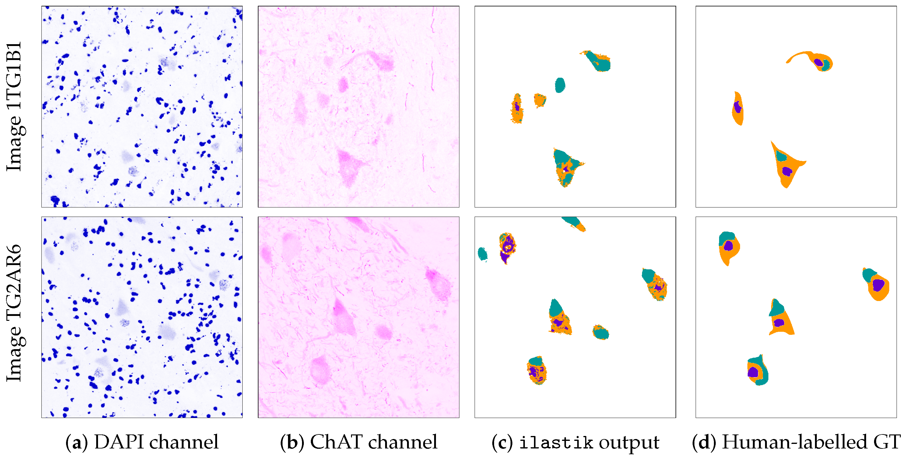
Since hand labelling in multi-class segmentation requires a huge amount of time, for the present work, we selected a subset of 90 representative images from the original ALS dataset. Each of these images was hand labelled by an expert, so as to generate hand-made, multi-class segmentations. These segmentations were used as the ground truth in the evaluation of the performance of ilastik and the USRL schema. In the remainder of this work, we refer to this dataset as the ALS-GT dataset, including the 90 tissue images and their hand-made segmentations. Figure 4 shows the channels DAPI and ChAT, respectively coloured in blue and magenta, for two images in the ALS-GT dataset, together with the segmentations produced by a human expert and ilastik. Ilastik was used as in the automated pipeline presented in Hagemann et al. [11].

3.2. Context-Specific Configuration of the USRL Schema

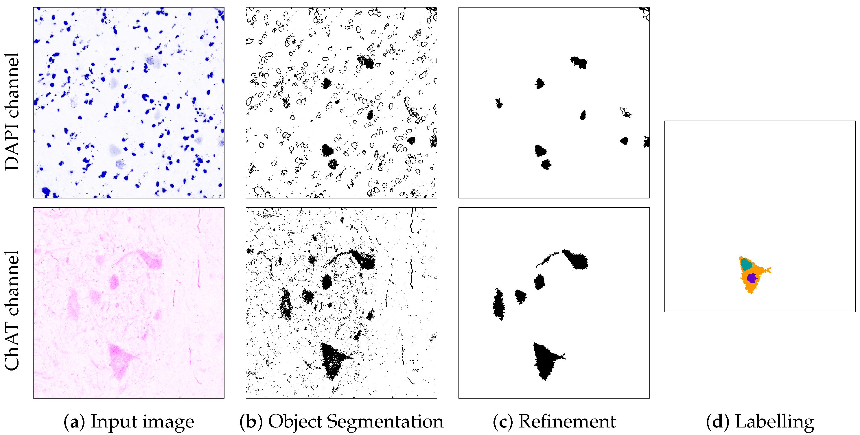
In Hagemann et al. [11], the authors analysed the images in the ALS dataset using the information contained in the DAPI and ChAT channels only. Following the same approach, only those two channels were considered in the instantiation of the USRL schema, MagNoLia (named after Motor Neuron Labeller); The software tool is available for download from https://github.com/giaracvi/MagNoLia (accessed on 24 April 2020) under the Apache 2.0 License. For a better visualisation of the process, the representation of the output of each phase is presented and explored in Figure 5.
The specific workflow of MagNoLia is set as follows:
(i)
Object Segmentation (OS) phase: OS is performed separately in the DAPI and in the ChAT channel. Regarding the DAPI channel, the aim is to segment the nuclei and inclusions of MNs. To that end, OS is performed with two techniques: thresholding and tone-based clustering. First, thresholding is used to alleviate the negative impact of very bright non-MN nuclei on the subsequent clustering; to that end, a tonal intensity threshold of 0.8 was imposed, considering only just the objects below that value. Next, tone-based clustering is based on the homogeneity of the inclusions and the MN nuclei, using k-means; the tones were separated into four different groups, and the two with medium intensities were selected.
Regarding the ChAT channel, the aim is to segment the MNs. With that intent, the OS is performed by self-adapting thresholding. Specifically, we used the Rosin method, as the unimodal tonal distribution in the image matched the thresholding priors of the method [23].
(ii)
Refinement phase: REF is performed separately in each of the channels. For the DAPI channel, we discarded those objects smaller than 0.05% of the area of the image. For the ChAT channel, REF is carried out similarly, just adapting the parameters (valid size range) to MN areas. In this case, the valid size was set to 0.12–10% of the area of the image, discarding any other object.
(iii)
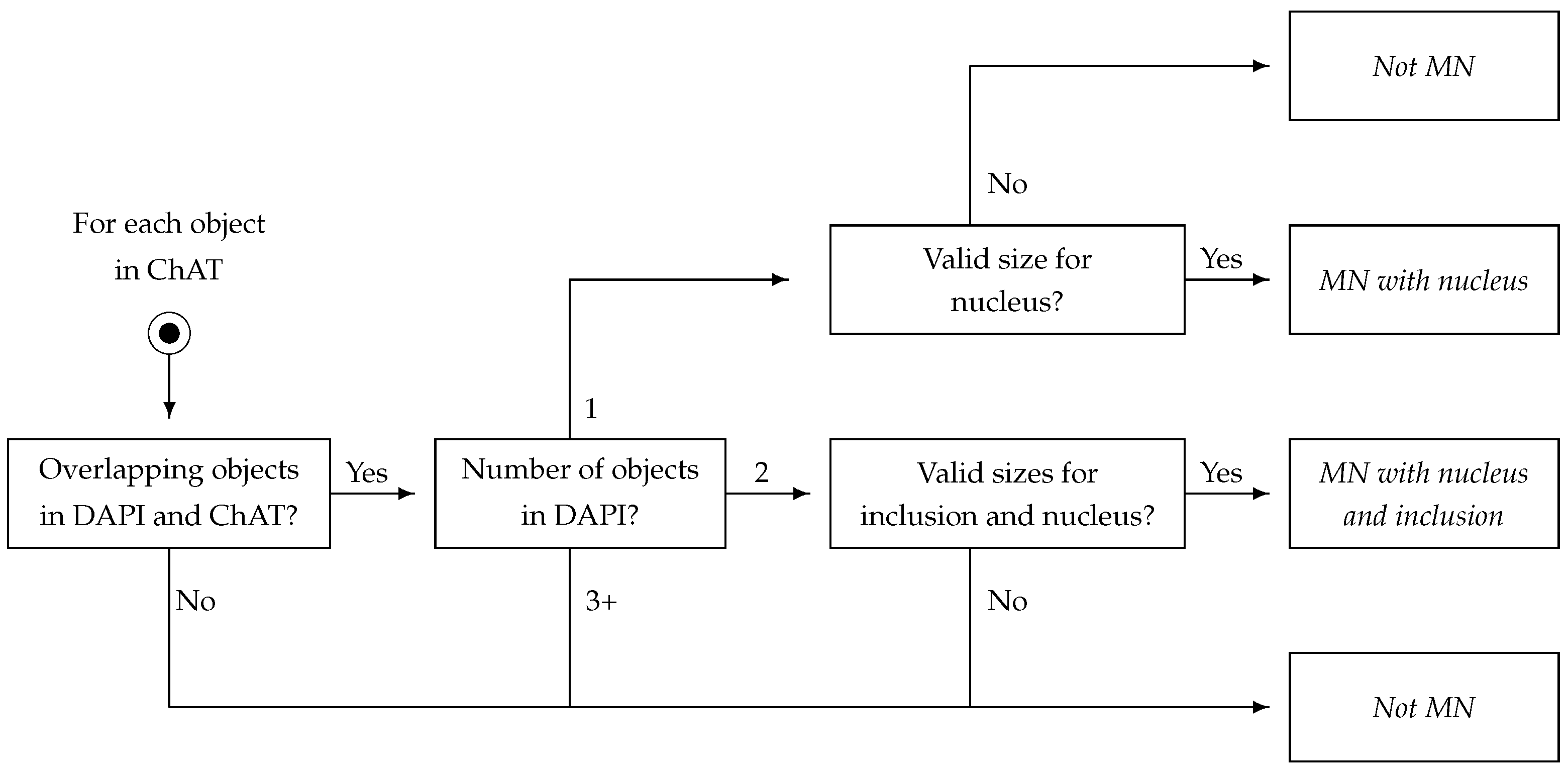
Labelling phase: The LBL phase combines the refined objects in DAPI and ChAT channels into a single representation. The process is depicted in Figure 6. For each object detected in ChAT, a series of questions are made. First, an object in ChAT is only considered as a candidate if it overlaps objects in DAPI; this corresponds to the idea that each MN must contain a nucleus, and might also contain an inclusion. An object in ChAT is considered valid if (a) it overlaps with an object in DAPI and (b) at least 90% of the area of such an object in DAPI is coincident with the object in ChAT. Applying this condition, the candidate objects are first categorised as an MN candidate with a nucleus (just one object in DAPI within an object in ChAT) or as an MN candidate with a nucleus and inclusion (two objects in DAPI within an object in ChAT). This decision was not based exclusively on the number of objects. The size was used as the second cascading decision, as no nucleus or inclusion can take up more than half of the area of a cell; specifically, DAPI objects must be greater than 5% and smaller than 50% of the ChAT object it overlaps. Note that, if the cell is finally recognised as an MN, each of its parts is individually labelled according to the appearance of its organelles in each of the channels.
The proposed schema of MagNoLia can not only be used for quantitative measures of the presence of cells, but also for the computation of topological (size, shape), biological (brightness) and, if a time series is available, even behavioural (speed, death) data.

4. Experiments

As explained in Section 3, MagNoLia is presented as an alternative for ilastik. In order to experimentally test its validity, both approaches were applied on the ALS-GT dataset, and the results were compared to the hand-labelled ground truth images. Section 4.1 elaborates on the comparison measures used, while Section 4.2 presents the actual comparison.

4.1. Quantitative Comparison Measures

Quality quantification in image processing tasks is relatively complex and usually requires a number of decisions on the type of data considered, as well as on the semantics and goals of the quantification itself. In this experiment, we intended to measure the visual proximity between the results generated by computer-based methods (MagNoLia and ilastik) and those by a human (the ground truth). Since these images were multi-class labelled, the problem would resemble a classical segmentation schema. The most popular alternatives for the comparison of multi-class images are based on multi-class confusion matrices, from which different scalar indices can be computed (see, e.g., the NPR by Unnikrishnan et al. [44]). One of the recurrent problems of multi-class confusion matrices relates to the quantitative weight (relevance) of each of the classes or of each of the potential misclassifications. It is, for example, unclear, whether all misclassifications are equally important or whether some mistakes are preferred over others.
In order to avoid excessive parameterization of the evaluation process, possibly hindering its interpretation, we designed a fourfold evaluation of the results in our experiments. First, we compared the quality of the results considering the whole MN, so as to represent the ability of the methods to detect the neurons. In this case, the multi-class labelled images were considered as binary images, where 1 s represent the MNs and 0s represent the background. Hence, the results are then compared as binary images. The same process was replicated for each of the three subregions of the MNs: nucleus, inclusion and cytoplasm. For each of such subregions, the results were converted into binary images, then compared. In this manner, we could compare the performance of each of the contending methods for (a) general MN detection and (b) the accurate detection of each of its components.
While the setup outlined is simpler than multi-class image comparison, it still requires a robust process of binary image comparison. Binary images are frequently used as a representation for intermediate or final outputs in image processing tasks. That is why binary images can be found in a broad range of applications, such as edge and saliency detection [45,46] and object segmentation and tracking [47,48]. The proliferation of the use of binary images in the image processing literature goes along with a rich variety of comparison measures to quantify their visual proximity; these measures provide a quantification of the similarity between two or more binary images (which can represent boundary maps, segmentations, etc.). The comparison of binary images can take different mathematical or morphological inspirations. Some have a metrical interpretation at the origin, a well-known example being the Hausdorff metric [49], which has subsequently evolved into Baddeley’s delta metric [50,51]. Other authors opt for a more geometrical interpretation of images [52] or translate the problem into an image matching task [53,54].
Popular comparison measures are based on the use of a confusion matrix [55,56,57], which allows considering both the coincident and the divergent information between two binary images, providing a very natural way to compare the prediction with the ground truth. In order to do so, the True Positives (TP), True Negatives (TN), False Positives (FP) and False Negatives (FN) were counted. Combining these values, different performance measures can be constructed, such as Rec and Prec:
Rec = TP TP + FN Prec = TP TP + FP ,
which are often combined into their harmonic mean, given by: F:
F = 2 · Rec · Prec Rec + Prec .
Note that Prec and Rec are preferred over other measures (as accuracy) because they avoid the use of TN. In the current dataset, as well as in most image processing tasks, most of the images contained no valid information, and so TN tended to be significantly larger than any other quantity in the confusion matrices. In order to avoid the distortion of the results by TN, we opted for Prec, Rec and F [54,58].

4.2. Results and Discussion

MagNoLia was applied to the ALS-GT image dataset presented in Section 3, an illustration of which was already shown in Figure 5. The biological restrictions imposed in the LBL phase were schematically represented in Figure 6, showing that the objects were either labelled as “MN with nucleus” or as “MN with nucleus and inclusion”. Figure 7 displays four images from the ALS-GT dataset, together with the segmentation by ilastik, MagNoLia and a human labeller. Note that, for a better visualisation of the original images, the DAPI and ChAT channels are combined here in different colour palettes, instead of being displayed separately.
Figure 7 points out some interesting facts. Overall, we can observe that MagNoLia labels a smaller number of objects than ilastik does. Furthermore, it is evident that ilastik does not enforce the cells to be biologically viable. Otherwise said, while the detection in MagNoLia forces the selected areas to represent viable MNs, the results by ilastik impose no such restriction. For example, ilastik labels some independent objects not contained in any MN as inclusions or nuclei. These cases are not labelled by MagNoLia, since they are biologically non-viable, due to the first condition in the LBL phase (“Overlapping objects in DAPI and ChAT?”). From a qualitative point of view, ilastik is likely to detect more MNs, at the cost of losing precision and confidence in the results. Even when comparing cases where both approaches failed, MagNoLia seemed to show a higher precision than ilastik.
Note that, in medical imaging, as experts deal with sensitive data, there is a preference to preserve only the most trustworthy information in image segmentation and classification processes, i.e., to preserve only what one is most confident about, even if that entails a loss of information in the process. This implies that restrictive methods are preferred over more permissive ones, since the latter, in order to account for more TP (obtaining a higher Rec), might also allow for more FP (entailing a lower Prec). Measures derived from a confusion matrix are well tailored for such an analysis and, consequently, were applied as performance measures to compare the results obtained by MagNoLia and ilastik with the hand-labelled ground truth.
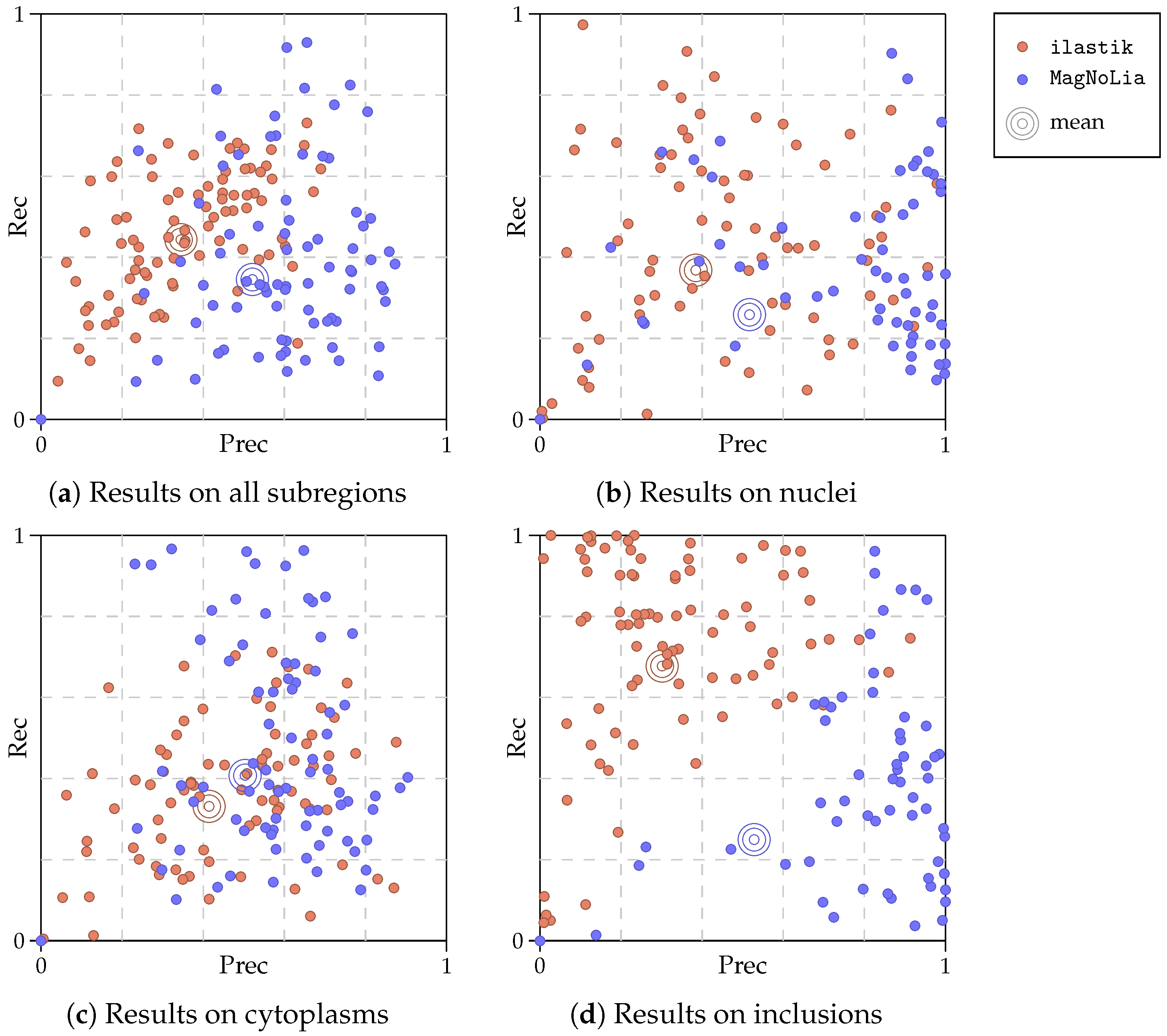
The quantitative comparison of the results is summarized in Table 1 and Table 2. In Table 1, we display the average Prec, Rec, and F for the global detection of MNs in the dataset, while Table 2 contains the results considering each individual subregion of the MNs. In this manner, Table 1 represents the global detection of MNs, and Table 2 illustrates the performance in finely detecting the components within them. Additionally, Figure 8 displays a more detailed view of the results in Table 1 and Table 2. Specifically, this figure displays the individual results (in terms of Prec and Rec) of each method and each image, as well as the mean for both ilastik and MagNoLia.
Regarding the global results in Table 1, we observed that MagNoLia had a higher Prec than ilastik. We can, hence, assert that MagNoLia meets the objective of providing a more trustworthy segmentation, which can be quantified in a 50% increment in Prec compared to ilastik. While less important than Prec, Rec is also a representative performance measure. As seen in Table 1, ilastik obtained a higher Rec, which means that it is in fact able to recognise and retrieve more objects than MagNoLia does. The trade-off between Rec and Prec can be visually seen on image 1TG1B1 in Figure 7a. In this image, while MagNoLia detects a single MN (and its contents), ilastik detects them all, at the cost of poor discrimination of spurious objects.
The results considering each of the individual parts of the cell were also favourable to MagNoLia. In fact, MagNoLia obtained a higher Prec for all possible subregions of the MNs. In fact, the improvement w.r.t. ilastik was significant, especially in the case of the inclusions. As was the case for the results in Table 1, ilastik is generally better than MagNoLia in terms of Rec, while both are comparable in terms of F.
A detailed view into the results is given in Figure 8. In this figure, we observe the distribution of the results that lead to the averaged quantities in Table 1 and Table 2. Overall, it was clear that MagNoLia tended to produce a greater precision than ilastik, at the cost of a lower recall. This can be clearly seen in Figure 8a, but also in the results for individual cell regions, especially in Figure 8c. A more detailed analysis brought forward facts that could not be seen in Table 1 and Table 2. Interestingly, ilastik tended to produce results grouped around the mean, while MagNoLia did not. While in Figure 8a,c, the mean result by MagNoLia is influenced by similar results for individual images, this is not the case in Figure 8b,d, where Prec tends to have extreme values for individual images.
Observing the results in Figure 8, the validity of the mean as the global evaluation of the results by each method might be questioned in favour of other alternatives (such as the median). However, the mean does embody the idea of measuring the amount of information obtained across the dataset. Discarding outliers, or using the median, might hinder the understanding of the amount of information retrieved by each of the methods across the dataset. It is, however, very relevant to know that the mean Prec obtained by MagNoLia was, occasionally, produced by a combination of very high and low results, not necessarily grouped around the mean (especially for the inclusions, as can be seen in Figure 8d).
As a general conclusion, we can state that MagNoLia provided better results than ilastik, given that Prec is preferred over Rec in the context of neural tissue analysis. In quantitative terms, MagNoLia succeeded in ensuring a higher precision than ilastik. Moreover, from a qualitative perspective, MagNoLia was also able to produce results that were better aligned with the biological requirements.

5. Conclusions

In this work, we presented a fully automated and unsupervised cell segmentation and identification schema for microscopy fluorescent images. Specifically, we outlined an unsupervised multi-phase schema (called the USRL schema), avoiding the necessity of labelling training data, thus reducing the experts’ workload. As a proof-of-principle, we applied an instantiation of this schema (called MagNoLia) to a dataset of ALS molecular pathology confocal images. However, MagNoLia can not only be applied to other immunostaining and tissue samples, as the USRL schema can also be instantiated for a large variety of other datasets and fields, from cancer pathology to basic cell biology analysis. In our proof-of-principle on the ALS dataset, we performed a comparison with a state-of-the-art machine learning segmentation tool called ilastik [14], summarised as Rec, Prec and F. As a conclusion, we can affirm that MagNoLia allows for an easy and intuitive incorporation of biological knowledge into the segmentation process, while providing more control to the experts. MagNoLia also yielded a higher Prec, yielding more trustworthy segmentations than ilastik did.

Author Contributions

Conceptualisation, D.G.-C., A.S. and C.L.-M.; methodology, D.G.-C., A.S., B.D.B. and C.L.-M.; software, S.I.-R. and F.A.-S.; validation, S.I.-R.; formal analysis, S.I.-R., H.B., B.D.B. and C.L.-M.; investigation, S.I.-R., F.A.-S. and C.L.-M.; resources, C.H., R.P. and A.S.; data curation, C.H., and R.P.; writing—original draft preparation, S.I.-R. and F.A.-S.; writing—review and editing, D.G.-C., A.S., B.D.B. and C.L.-M.; visualisation, C.H., S.I.-R. and F.A.-S.; supervision, D.G.-C., A.S., B.D.B. and C.L.-M.; project administration, D.G.-C., H.B., A.S. and C.L.-M.; funding acquisition, D.G.-C., H.B., A.S. and C.L.-M. All authors read and agreed to the published version of the manuscript.

Funding

This research received no external funding.

Institutional Review Board Statement

Not applicable.

Informed Consent Statement

Not applicable.

Data Availability Statement

Not applicable.

Acknowledgments

The authors gratefully acknowledge the financial support of the Spanish Ministry of Science (Project PID2019-108392GB-I00 AEI/FEDER, UE), the funding from the European Union’s H2020 research and innovation programme under Marie Sklodowska-Curie Grant Agreement Number 801586, as well as that of Navarra de Servicios y Tecnologías, S.A. (NASERTIC). A.S. and C.H. wish to acknowledge the support of King’s College London (Studentship “LAMBDA: long axons for motor neurons in a bioengineered model of ALS” from FoDOCS) and the Wellcome Trust (213949/Z/18/Z). On behalf of A.S., C.H. and R.P., this research was funded in whole, or in part, by the Wellcome Trust (213949/Z/18/Z). For the purposes of open access, the authorhas applied a CC BY public copyright licence to any author-accepted manuscript version arising from this submission.

Conflicts of Interest

The authors declare no conflict of interest.

Abbreviations

The following abbreviations are used in this manuscript:
NDsNeurodegenerative Diseases
USRLUnsupervised Segmentation Refinement Labelling
OSObject Segmentation
REFRefinement
LBLLabelling
MNMotor Neuron

References

  1. Przedborski, S.; Vila, M.; Jackson-Lewis, V. Series Introduction: Neurodegeneration: What is it and where are we? J. Clin. Investig. 2003, 111, 3–10. [Google Scholar] [CrossRef] [Green Version]
  2. Masters, C.; Bateman, R.; Blennow, K.; Rowe, C.; Sperling, R.; Cummings, J. Alzheimer’s disease. Nat. Rev. Dis. Prim. 2015, 1, 15056. [Google Scholar] [CrossRef]
  3. Hardiman, O.; Al-Chalabi, A.; Chió, A.; Corr, E.; Logroscino, G.; Robberecht, W.; Shaw, P.; Simmons, Z.; Berg, L. Amyotrophic lateral sclerosis. Nat. Rev. Dis. Prim. 2017, 3, 17085. [Google Scholar] [CrossRef]
  4. Poewe, W.; Seppi, K.; Tanner, C.; Halliday, G.; Brundin, P.; Volkmann, J.; Schrag, A.E.; Lang, A. Parkinson disease. Nat. Rev. Dis. Prim. 2017, 3, 17013. [Google Scholar] [CrossRef]
  5. Hou, Y.; Dan, X.; Babbar, M.; Wei, Y.; Hasselbalch, S.; Croteau, D.; Bohr, V. Ageing as a risk factor for neurodegenerative disease. Nat. Rev. Neurol. 2019, 15, 565–581. [Google Scholar] [CrossRef] [PubMed]
  6. Abraham, V.C.; Taylor, D.L.; Haskins, J.R. High content screening applied to large-scale cell biology. Trends Biotechnol. 2004, 22, 15–22. [Google Scholar] [CrossRef] [PubMed]
  7. Boutros, M.; Heigwer, F.; Laufer, C. Microscopy-based high-content screening. Cell 2015, 163, 1314–1325. [Google Scholar] [CrossRef] [Green Version]
  8. Arrasate, M.; Finkbeiner, S. Automated microscope system for determining factors that predict neuronal fate. Proc. Natl. Acad. Sci. USA 2005, 102, 3840–3845. [Google Scholar] [CrossRef] [Green Version]
  9. Serio, A.; Bilican, B.; Barmada, S.J.; Ando, D.M.; Zhao, C.; Siller, R.; Burr, K.; Haghi, G.; Story, D.; Nishimura, A.L.; et al. Astrocyte pathology and the absence of non-cell autonomy in an induced pluripotent stem cell model of TDP-43 proteinopathy. Proc. Natl. Acad. Sci. USA 2013, 110, 4697–4702. [Google Scholar] [CrossRef] [Green Version]
  10. Hall, C.E.; Yao, Z.; Choi, M.; Tyzack, G.E.; Serio, A.; Luisier, R.; Harley, J.; Preza, E.; Arber, C.; Crisp, S.J.; et al. Progressive motor neuron pathology and the role of astrocytes in a human stem cell model of VCP-related ALS. Cell Rep. 2017, 19, 1739–1749. [Google Scholar] [CrossRef] [Green Version]
  11. Hagemann, C.; Tyzack, G.E.; Taha, D.M.; Devine, H.; Greensmith, L.; Newcombe, J.; Patani, R.; Serio, A.; Luisier, R. Automated and unbiased discrimination of ALS from control tissue at single cell resolution. Brain Pathol. 2021, e12937. [Google Scholar] [CrossRef]
  12. Tyzack, G.E.; Luisier, R.; Taha, D.M.; Neeves, J.; Modic, M.; Mitchell, J.S.; Meyer, I.; Greensmith, L.; Newcombe, J.; Ule, J.; et al. Widespread FUS mislocalization is a molecular hallmark of ALS. Brain 2019, 142, 2572–2580. [Google Scholar] [CrossRef] [PubMed] [Green Version]
  13. Íñigo Marco, I.; Valencia, M.; Larrea, L.; Bugallo, R.; Martínez-Goikoetxea, M.; Zuriguel, I.; Arrasate, M. E46K α-synuclein pathological mutation causes cell-autonomous toxicity without altering protein turnover or aggregation. Proc. Natl. Acad. Sci. USA 2017, 39, E8274–E8283. [Google Scholar] [CrossRef] [Green Version]
  14. Berg, S.; Kutra, D.; Kroeger, T.; Straehle, C.; Kausler, B.; Haubold, C.; Schiegg, M.; Ales, J.; Beier, T.; Rudy, M.; et al. Ilastik: Interactive machine learning for (bio)image analysis. Nat. Methods 2019, 16, 1226–1232. [Google Scholar] [CrossRef] [PubMed]
  15. Friebel, A.; Neitsch, J.; Johann, T.; Hammad, S.; Hengstler, J.G.; Drasdo, D.; Hoehme, S. TiQuant: Software for tissue analysis, quantification and surface reconstruction. Bioinformatics 2015, 31, 3234–3236. [Google Scholar] [CrossRef] [Green Version]
  16. Carpenter, A.; Jones, T.; Lamprecht, M.; Clarke, C.; Kang, I.; Friman, O.; Guertin, D.; Chang, J.; Lindquist, R.; Moffat, J.; et al. CellProfiler: Image analysis software for identifying and quantifying cell phenotypes. Genome Biol. 2006, 7, R100. [Google Scholar] [CrossRef] [Green Version]
  17. Myszczynska, M.A.; Ojamies, P.N.; Lacoste, A.M.; Neil, D.; Saffari, A.; Mead, R.; Hautbergue, G.M.; Holbrook, J.D.; Ferraiuolo, L. Applications of machine learning to diagnosis and treatment of neurodegenerative diseases. Nat. Rev. Neurol. 2020, 16, 440–456. [Google Scholar] [CrossRef]
  18. Krizhevsky, A.; Sutskever, I.; Hinton, G.E. Imagenet classification with deep convolutional neural networks. Adv. Neural Inf. Process. Syst. 2012, 25, 1097–1105. [Google Scholar] [CrossRef]
  19. Breiman, L. Random forests. Mach. Learn. 2001, 45, 5–32. [Google Scholar] [CrossRef] [Green Version]
  20. Rudin, C. Stop explaining black box machine learning models for high stakes decisions and use interpretable models instead. Nat. Mach. Intell. 2019, 1, 206–215. [Google Scholar] [CrossRef] [Green Version]
  21. Weiss, K.; Khoshgoftaar, T.; Wang, D. A survey of transfer learning. J. Big Data 2016, 3, 1345–1359. [Google Scholar] [CrossRef] [Green Version]
  22. Otsu, N. Threshold selection method for gray-level histograms. IEEE Trans. Syst. Man Cybern. 1979, 9, 62–66. [Google Scholar] [CrossRef] [Green Version]
  23. Rosin, P.L. Unimodal thresholding. Pattern Recognit. 2001, 34, 2083–2096. [Google Scholar] [CrossRef]
  24. Ramírez-Ortegón, M.A.; Tapia, E.; Rojas, R.; Cuevas, E. Transition thresholds and transition operators for binarization and edge detection. Pattern Recognit. 2010, 43, 3243–3254. [Google Scholar] [CrossRef]
  25. Su, B.; Lu, S.; Tan, C.L. Robust document image binarization technique for degraded document images. IEEE Trans. Image Process. 2012, 22, 1408–1417. [Google Scholar]
  26. Tomasi, C.; Manduchi, R. Bilateral filtering for gray and color images. In Proceedings of the IEEE International Conference on Computer Vision, Bombay, India, 7 January 1998; pp. 838–846. [Google Scholar]
  27. Weickert, J. Anisotropic Diffusion in Image Processing; ECMI Series; Teubner-Verlag: Stuttgart, Germany, 1998. [Google Scholar]
  28. Barash, D. A Fundamental Relationship between Bilateral Filtering, Adaptive Smoothing, and the Nonlinear Diffusion Equation. IEEE Trans. Pattern Anal. Mach. Intell. 2002, 24, 844–847. [Google Scholar] [CrossRef] [Green Version]
  29. Lopez-Molina, C.; Galar, M.; Bustince, H.; De Baets, B. On the impact of anisotropic diffusion on edge detection. Pattern Recognit. 2014, 47, 270–281. [Google Scholar] [CrossRef]
  30. Wang, G.; Lopez-Molina, C.; De Baets, B. Automated blob detection using iterative Laplacian of Gaussian filtering and unilateral second-order Gaussian kernels. Digit. Signal Process. 2020, 96, 102592. [Google Scholar] [CrossRef]
  31. Achanta, R.; Shaji, A.; Smith, K.; Lucchi, A.; Fua, P.; Süsstrunk, S. SLIC superpixels compared to state-of-the-art superpixel methods. IEEE Trans. Pattern Anal. Mach. Intell. 2012, 34, 2274–2282. [Google Scholar] [CrossRef] [Green Version]
  32. Duda, R.O.; Hart, P.E. Use of the Hough transformation to detect lines and curves in pictures. Commun. ACM 1972, 15, 11–15. [Google Scholar] [CrossRef]
  33. Wang, G.; Lopez-Molina, C.; De Baets, B. High-ISO Long-Exposure Image Denoising Based on Quantitative Blob Characterization. IEEE Trans. Image Process. 2020, 29, 5993–6005. [Google Scholar] [CrossRef]
  34. Belongie, S.; Malik, J.; Puzicha, J. Shape matching and object recognition using shape contexts. IEEE Trans. Pattern Anal. Mach. Intell. 2002, 24, 509–522. [Google Scholar] [CrossRef] [Green Version]
  35. Mokhtarian, F.; Mackworth, A.K. A theory of multiscale, curvature-based shape representation for planar curves. IEEE Trans. Pattern Anal. Mach. Intell. 1992, 14, 789–805. [Google Scholar] [CrossRef]
  36. Haralick, R.M.; Sternberg, S.R.; Zhuang, X. Image Analysis Using Mathematical Morphology. IEEE Trans. Pattern Anal. Mach. Intell. 1987, 9, 532–550. [Google Scholar] [CrossRef] [PubMed]
  37. Bibiloni, P.; González-Hidalgo, M.; Massanet, S. A real-time fuzzy morphological algorithm for retinal vessel segmentation. J. Real Time Image Process. 2019, 16, 2337–2350. [Google Scholar] [CrossRef]
  38. Haralick, R.M.; Shanmugam, K.; Dinstein, I.H. Textural features for image classification. IEEE Trans. Syst. Man Cybern. 1973, 3, 610–621. [Google Scholar] [CrossRef] [Green Version]
  39. Canny, J. A computational approach to edge detection. IEEE Trans. Pattern Anal. Mach. Intell. 1986, 8, 679–698. [Google Scholar] [CrossRef] [PubMed]
  40. Schneider, A.F.L.; Hackenberger, C.P.R. Fluorescent labelling in living cells. Curr. Opin. Biotechnol. 2017, 48, 61–68. [Google Scholar] [CrossRef]
  41. Cheng, H.D.; Chen, C.; Chiu, H.; Xu, H. Fuzzy homogeneity approach to multilevel thresholding. IEEE Trans. Image Process. 1998, 7, 1084–1086. [Google Scholar] [CrossRef]
  42. Tang, J.; Peli, E.; Acton, S. Image enhancement using a contrast measure in the compressed domain. IEEE Signal Process Lett. 2003, 10, 289–292. [Google Scholar] [CrossRef]
  43. Hung, M.C.; Link, W. Protein localization in disease and therapy. J. Cell Sci. 2011, 124, 3381–3392. [Google Scholar] [CrossRef] [Green Version]
  44. Unnikrishnan, R.; Pantofaru, C.; Hebert, M. Toward objective evaluation of image segmentation algorithms. IEEE Trans. Pattern Anal. Mach. Intell. 2007, 29, 929–944. [Google Scholar] [CrossRef] [PubMed] [Green Version]
  45. Sun, G.; Liu, Q.; Liu, Q.; Ji, C.; Li, X. A novel approach for edge detection based on the theory of universal gravity. Pattern Recognit. 2007, 40, 2766–2775. [Google Scholar] [CrossRef]
  46. Goferman, S.; Zelnik-Manor, L.; Tal, A. Context-aware saliency detection. IEEE Trans. Pattern Anal. Mach. Intell. 2012, 34, 1915–1926. [Google Scholar] [CrossRef] [PubMed] [Green Version]
  47. Arbelaez, P.; Maire, M.; Fowlkes, C.; Malik, J. Contour Detection and Hierarchical Image Segmentation. IEEE Trans. Pattern Anal. Mach. Intell. 2011, 33, 898–916. [Google Scholar] [CrossRef] [Green Version]
  48. Yokoyama, M.; Poggio, T. A contour-based moving object detection and tracking. In Proceedings of the International Workshop on Visual Surveillance and Performance Evaluation of Tracking and Surveillance, Beijing, China, 15–16 October 2005; pp. 271–276. [Google Scholar]
  49. Sim, D.G.; Kwon, O.K.; Park, R.H. Object matching algorithms using robust Hausdorff distance measures. IEEE Trans. Image Process. 1999, 8, 425–429. [Google Scholar] [PubMed]
  50. Baddeley, A.J. An error metric for binary images. In Robust Computer Vision: Quality of Vision Algorithms; Wichmann Verlag: Karlsruhe, Germany, 1992. [Google Scholar]
  51. Brunet, D.; Sills, D. A Generalized Distance Transform: Theory and Applications to Weather Analysis and Forecasting. IEEE Trans. Geosci. Remote Sens. 2017, 55, 1752–1764. [Google Scholar] [CrossRef]
  52. Gimenez, J.; Martinez, J.; Flesia, A.G. Unsupervised edge map scoring: A statistical complexity approach. Comput. Vis. Image Underst. 2014, 122, 131–142. [Google Scholar] [CrossRef] [Green Version]
  53. Estrada, F.J.; Jepson, A.D. Quantitative evaluation of a novel image segmentation algorithm. In Proceedings of the IEEE Conference on Computer Vision and Pattern Recognition, San Diego, CA, USA, 20–26 June 2005; Volume 2, pp. 1132–1139. [Google Scholar]
  54. Martin, D.; Fowlkes, C.; Malik, J. Learning to detect natural image boundaries using local brightness, color, and texture cues. IEEE Trans. Pattern Anal. Mach. Intell. 2004, 26, 530–549. [Google Scholar] [CrossRef]
  55. Warfield, S.K.; Zou, K.H.; Wells, W.M. Simultaneous truth and performance level estimation (STAPLE): An algorithm for the validation of image segmentation. IEEE Trans. Med. Imaging 2004, 23, 903–921. [Google Scholar] [CrossRef] [Green Version]
  56. Asman, A.; Landman, B. Robust Statistical Label Fusion through Consensus Level, Labeler Accuracy and Truth Estimation (COLLATE). IEEE Trans. Med. Imaging 2011, 30, 1779–1794. [Google Scholar] [CrossRef] [PubMed] [Green Version]
  57. Lopez-Molina, C.; De Baets, B.; Bustince, H. Quantitative error measures for edge detection. Pattern Recognit. 2013, 46, 1125–1139. [Google Scholar] [CrossRef]
  58. Lopez-Molina, C.; Marco-Detchart, C.; Bustince, H.; De Baets, B. A survey on matching strategies for boundary image comparison and evaluation. Pattern Recognit. 2021, 115, 107883. [Google Scholar] [CrossRef]
Figure 1. Visual representation of the USRL schema workflow: (a) the original USRL schema input image; (b) the output resulting from the object segmentation phase; (c) the refinement output of (b), eliminating unwanted objects and noise; (d) the final labelled image, where each class comes with an associated colour.
Applsci 11 03733 g001
Figure 2. Schematic representation of the USRL schema. Each phase is depicted by a rectangle, with the information flow being represented by arrows.
Applsci 11 03733 g002
Figure 3. Original images from the ALS dataset, all from the same tissue observation, where: (a) is the image from Channel 1 (DAPI); (b) is the Channel 2 (SFPQ) image; (c) contains the Channel 3 (ChAT) image; and (d) shows the Channel 4 (FUS) image.
Applsci 11 03733 g003
Figure 4. Two examples of MN segmentation and labelling using ilastik. Each example takes up one row. For each example, the columns display (a,b) channels DAPI (coloured in blue) and ChAT (coloured in magenta) in the original image, (c) the result of the segmentation using ilastik and (d) the Ground Truth (GT) generated by an expert for that same image. In Columns (c,d), teal pixels represent inclusions, orange ones represent cytoplasms and purple ones represent nuclei.
Applsci 11 03733 g004
Figure 5. Visualisation of the output of each of the phases of MagNoLia for Image 1TG1B1. The segmentation is restricted to two channels, the DAPI and ChAT. Column (a) represents the original DAPI (coloured in blue) and ChAT (coloured in magenta) inputs; Columns (bd) display the output of the object segmentation, refinement and labelling phases, respectively.
Applsci 11 03733 g005
Figure 6. Schematic representation of the Labelling (LBL) phase for each object in MagNoLia. Boxes with slanted text represent final states, while all remaining boxes are decision nodes.
Applsci 11 03733 g006
Figure 7. Visual representation of the output by ilastik, MagNoLia and human experts for four different images in the dataset. Each row contains the results for a single image. Column (a) displays an overlap of the DAPI (coloured in blue) and ChAT (coloured in magenta) channels; Columns (bd) display the output by ilastik, MagNoLia and the human labeller, respectively. In Columns (bd), teal pixels represent inclusions, orange ones represent cytoplasms and purple ones represent nuclei.
Applsci 11 03733 g007
Figure 8. Distribution of results for ilastik and MagNoLia according to the type of subregion. Plot (a) represents the Prec and Rec for all subregions, while Plots (bd) represent the precision and recall of each subregion of an MN. The concentric circles represent, for each plot, the mean (centre of mass) of the point clouds.
Applsci 11 03733 g008
Table 1. Average quantitative results obtained by ilastik and MagNoLia on the images in the ALS-GT dataset for the segmentation of MNs. Each row corresponds to a different performance measure, and the best results for each performance measure are put in boldface for better visualisation.
ilastikmagnolia
Prec0.3460.537
Rec0.4670.324
F0.3980.404
Table 2. Average quantitative results obtained by ilastik and MagNoLia on the images in the ALS-GT dataset for the segmentation of each subregion of an MN. Each row corresponds to a different performance measure, and the best results for each type of subregion and performance measure are put in boldface for better visualisation.
NucleiCytoplasmsInclusions
ilastikMagNoLiailastikMagNoLiailastikMagNoLia
Prec0.3480.4380.4390.5130.2860.689
Rec0.3900.2380.3640.3750.6970.269
F0.3670.3080.3980.4330.4060.387
Publisher’s Note: MDPI stays neutral with regard to jurisdictional claims in published maps and institutional affiliations.