New Protocol and Architecture for a Wastewater Treatment System Intended for Irrigation

Abstract

Water quality may be affected by aspects such as pollution from industries, agricultural fertilizers and pesticides, and waste produced by humans. This contamination can affect the produce of the fields irrigated by untreated water. Therefore, it is necessary to add a treatment process in irrigation systems. In this paper, an architecture, communication protocol, and a data analysis algorithm for a wastewater treatment system intended for irrigation are presented. Our system includes a smart group-based wireless sensor network that is able to detect high salinity levels and pollution stains, such as oil spills. When contamination is detected, the water is led into auxiliary canals that perform the biosorption process to treat the water and dump it back into the main canal. Simulations were performed to assess the amount of data stored on the secure digital (SD) card, the consumed bandwidth, and the energy consumption of our proposal. The results show the system has a low bandwidth consumption with a maximum of 2.58 kbps for the setting of two daily data transmissions of the node in the last auxiliary canal. Furthermore, it can sustain the energy consumption in adverse conditions, where the node with the highest energy consumption reaches the lowest energy value of 12,320 mW/h.

1. Introduction

As a great part of agricultural produce is intended for human consumption, the quality of the water utilized for irrigation is essential. However, water quality may be affected by many aspects such as pollution from industries, agricultural fertilizers and pesticides, and waste produced by humans. UNESCO estimates the amount of contaminated water on the planet as 12,000 km³ [1]. Poorer regions of the planet are the most affected by contaminated water. Contaminated water is able to cause numerous health problems in the population. The WHO estimates the number of deaths caused by contaminated water consumption to be 842,000 [2]. Furthermore, it is estimated that there are 200,000 deaths per year due to pesticide consumption, with nearly 3 million people poisoned per year [3]. In India, 29% of the pesticide consumption is used on rice and 9% is used on vegetables. Thus, it is imperative to assure irrigation water is treated correctly so as to reduce water pollution as much as possible.

Considering the repercussions of water contamination on people, it is necessary to add a treatment process in irrigation systems. Even though irrigation water may have been treated prior to distribution, the characteristics of the distribution canals may not avoid the incursion of water pollutants during water transport. There are a variety of water treatment processes, including advanced oxidation processes (AOPs) [4], and adsorption, both organic and inorganic, among other water treatment processes [5]. Biosorption is a physical wastewater treatment that employs biomass to adsorb chemicals, metals, and other pollutants [6]. This process may employ different types of biomass such as marine algae, bacteria, fungi, peat moss, bark, and yeast and each type may present better results with different types of pollutants [7]. Agricultural waste materials are also being considered as an economic and ecologic biomass source. Agricultural waste biomass is abundant, reduces the waste generated from agriculture, and it has a low cost and high efficiency as an absorbent. Some of the already tested agricultural waste biomass absorbents are sawdust, coconut shells, rice bran, wheat bran, sugarcane bagasse, sugar beet pulp, maize corn cob, orange peels, waste tea leaves, and hazelnut shells, among other agricultural waste from different produce types [8]. The remnant of the wastewater biosorption process is treated with anaerobic digestion, dewatering, incineration, thermal drying, or pyrolysis [9].

In order to include water treatment in irrigation systems, an evaluation of the quality of the water that reaches the irrigation system must be performed before irrigation. Water quality monitoring can be performed with chemical or physical sensors. Physical sensors allow monitoring water quality in real time and do not require continuous supervision and manipulation. Thus, physical water quality monitoring sensors are suitable for remote water quality monitoring in smart irrigation systems. Physical sensors use the electromagnetic field, optical properties, and resistance variations in order to assess changes in the characteristics of the monitored environment [10]. Therefore, optical sensors can be utilized to monitor turbidity or the presence of an oil layer. Coils can be employed to determine the conductivity of the water. Moreover, image processing performed on the images obtained from cameras can be utilized to detect the presence of objects or animals. Furthermore, currently available low-cost sensors can be used to monitor water quality, with results comparable to those obtained from more expensive commercialized probes for water quality assessment.

The amount of information generated from these types of sensors and smart systems applied to precision agriculture can be significantly large. Thus, data processing algorithms are necessary to analyze the data and determine the actions that the actuators must perform. These algorithms may also consider reducing the amount of forwarded data in order to reduce energy consumption and the amount of generated traffic. Fault tolerance is another aspect that is usually considered by the algorithms employed in wireless sensor networks (WSNs) and Internet of Things (IoT) solutions. Moreover, some solutions consider soil moisture and other factors such as weather predictions to determine whether the irrigation system must start or stop [11].

In this paper, a communication protocol and a data analysis algorithm for a wastewater treatment system intended for irrigation are presented. Our system includes a smart group-based wireless sensor network that is able to detect, locate, monitor, and track high salinity levels and pollution stains, such as oil spills. Moreover, a new kind of water treatment plant is proposed to depollute the water before the irrigation. The system will use artificial intelligence techniques and data fusion methodologies in order to quantify the amount of pollution in the source and to detect and predict its movement and form. These techniques will allow the system to be conscious of what is happening in the water environment and send alarms through the warning system. This information will be used to define one treatment or other before using the water for smart irrigation.

The rest of the paper is organized as follows. The description of our proposal is given in Section 2. The results are presented in Section 3. Section 4 discusses the related work. Finally, the conclusion and future work are presented in Section 5.

2. Materials and Methods

In this section, the different nodes, sensors, and actuators proposed to collect data from the field and carry out the corresponding actions that allow treating the water are described. Furthermore, the architecture, the proposed communication protocol, and a data analysis algorithm for a wastewater treatment system intended for irrigation are presented.

2.1. Node Description

In this subsection, the description of the characteristics of the node, the sensors, and the actuators are performed.

In our proposed system, the nodes are deployed throughout the expanse of the canals, both for urban areas and farming areas. The quantity of nodes depends on the number of canals and their specific needs. The employed nodes are Arduino Mega 2560 [12]. The node has 16 analog input pins and 54 digital input/output pins, allowing for connecting many sensors to one single node. Moreover, it provides a universal serial bus (USB) connection, 4 universal asynchronous receiver-transmitter (UART) serial ports, a power jack, a 16 MHz crystal oscillator, an in-circuit serial programming (ICSP) header, and a reset button. However, as the node does not provide an integrated wireless interface, it is necessary to incorporate wireless modules. The nodes can be provided with long-range wide area network (LoRaWAN) connectivity by employing the module F8L10D-N [13] which transmits in the 868 Mhz band.

The sensor used to monitor water quality will be used to monitor turbidity and conductivity. For the detection of turbidity, optical sensors are used, while for conductivity monitoring, inductive sensors are used. The turbidity sensor is based on that presented in [14]. It is made with two light emitting diodes (LED) that emit at different wavelengths and two light detectors. One of the LEDs has a maximum wavelength of 612–625 nm and the other of 850 nm. The light detectors are a light-dependent resistor (LDR) that responds to the visible light of the first LED and a photodiode that responds to the infrared (IR) light of the second LED. The turbidity sensor is placed before and after the application of the filters to treat the water. The LEDs are powered at 3.3 V using the 3.3 V output voltage.

The conductivity sensor is based on the prototype described in [10]. It is composed of two copper coils. The first coil is powered with a sine wave and the second coil is induced. The induced voltage depends on the conductivity of the water. The powered coil is powered with the Arduino using an analog output (PWM) pin. The generated voltage in the induced coil is measured. Both the turbidity sensor and the conductivity sensor are connected to the same node. They are placed before and after the filters and will monitor the correct operation of the wastewater treatment filters by registering the changes in water quality. Additionally, we use a sensor to detect the presence of hydrocarbon in the water. The sensor is based on the photoluminescence effect linked to the hydrocarbons. In the design of the sensor, different light colors are used to excite the molecules of a hydrocarbon. The light source is an LED and a photodetector is used as a receptor of the emitted light.

In order to execute the actions determined by the system, some nodes need to include an actuator. As an actuator connected to an Arduino node, a linear actuator can be utilized. The linear actuator is a device that converts the rotational motion of a low-voltage direct current (DC) motor into linear motion. This device can be utilized to open and close the gate for controlling the water in the canal.

2.2. Architecture

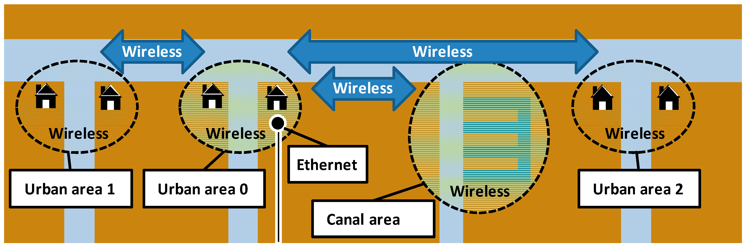
In this subsection, the proposed architecture is presented. The example of the area where the nodes are to be deployed is presented in Figure 1. As it can be seen in the image, there are several urban areas. These areas are zones with a population that may discharge wastewater into the canals that transport the water to the fields and is therefore subject to spill control. Furthermore, these areas have access to the electricity grid and the telecommunications infrastructure. The other area is the canal area. This area is located in an irrigation canal that leads to the fields. As it can be seen, in the canal areas, there is a comb-shaped structure that is formed by auxiliary canals that are connected with one another and have several gates that connect to the main canal. These auxiliary canals are prepared to implement the biosorption process that treats the water and removes contamination.

The sensor nodes deployed within the different zones communicate through wireless connections. Moreover, the communication between each of the zones is established wirelessly as well. In one of the urban areas, which in Figure 2 is called Urban Area 0, the gateway will establish a wired connection to transmit the data to the data center for storage and data analysis. The data that are received with information from the different nodes will be treated with artificial intelligence (AI), to respond with appropriate measures in our system. Lastly, the adopted measures will be forwarded to the actuator nodes to let the contaminated water go through the biosorption process.

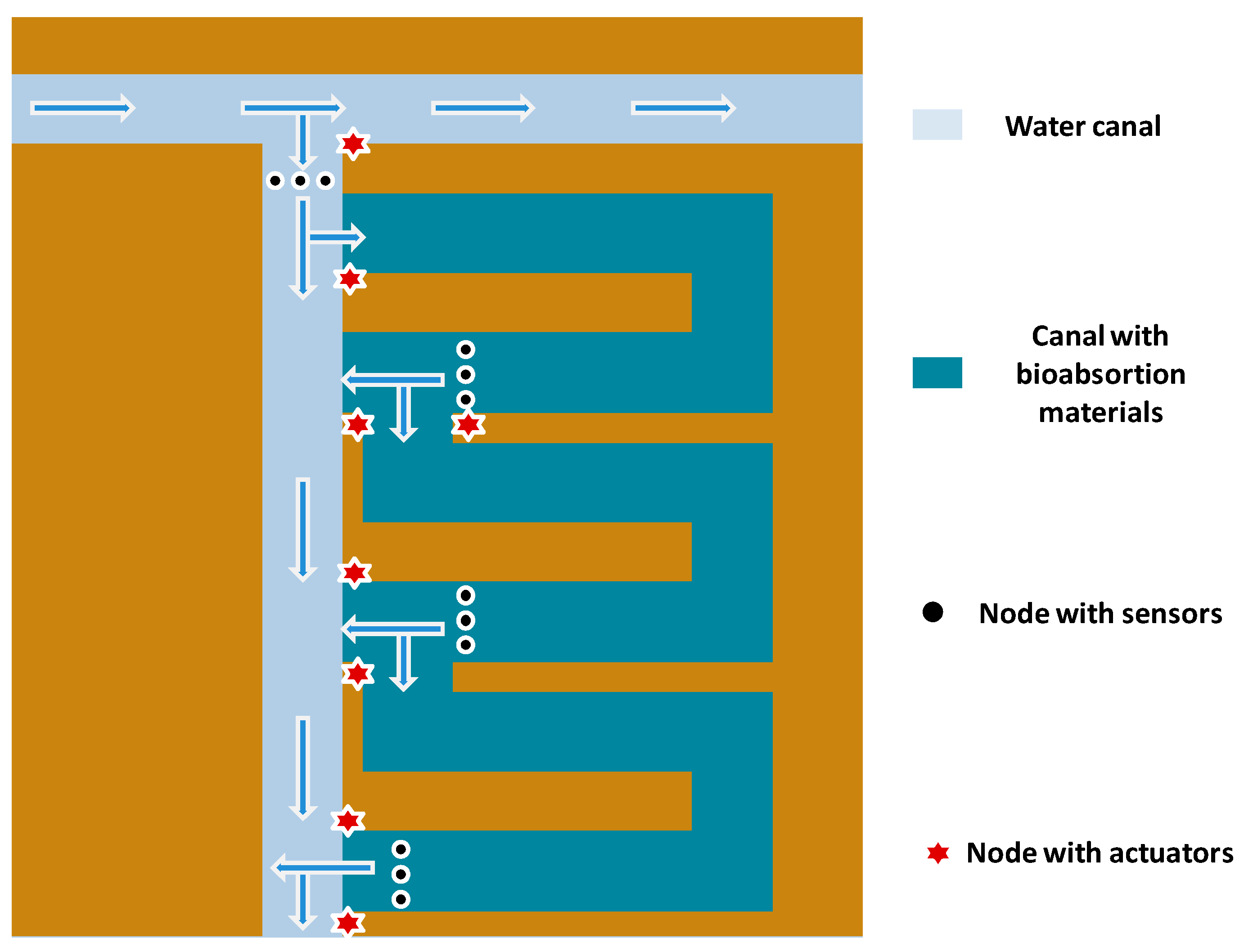
Figure 2 allows for visualizing in greater detail the location of the nodes in one of the canal zones. As can be seen, there are nodes to which different types of sensors and actuators are connected. Several auxiliary canals are found as well. These are comb-shaped canals where the biomass is located. The biomass is responsible for the decontamination of the water. As seen in the image, the biomass canals are replicated and connected, so the water can go through one or several decontamination phases, depending on the results of the samples obtained by the sensors, which are located at the end of each biomass canal. The actuator nodes are connected to lock-gates that allow for regulating the passage of the water flow.

The proposed architecture, formed by three layers, being Nodes Sensors & Actuators, Storage & Activation, and Artificial Intelligence, is shown in Figure 3. In the Nodes, Sensors & Actuators layer, all the nodes of the network are located. The different sensors that take measures of the water quality are connected to the nodes. Then, the data are periodically forwarded to the data center situated in the upper layer, where the data are stored. Furthermore, the actuators are connected to the nodes that are located at the gates of the canals so that the appropriate actions that have been decided in the higher layers are performed.

On the other hand, the Storage & Activation layer hosts the devices where the information received from all the sensors is stored. Furthermore, this layer also hosts the system that allows for sending orders to the actuators so as to carry out the actions established by the decision-making process that is performed in the upper layer.

Lastly, the systems that allow for processing the data that were stored in the lower layer are located in the Artificial Intelligence layer. This layer oversees the decision-making process whose result will be sent to the action functionality in the lower layer.

The protocol stack is presented in Figure 4. As it can be seen, the Network Interface layer uses an ethernet protocol in the wired network, and a LoRaWAN protocol to perform wireless transmissions. The wired network is based on the stack defined by the transmission control protocol/internet protocol (TCP/IP) reference model. IPv4 and IPv6 protocols are used in the Network layer. The protocols TCP and user datagram protocol (UDP) are used in the Transport layer. Finally, the Application layer can use any protocol of this layer to implement the proposed system. On the other hand, for the wireless network, the physical layer utilizes the LoRa modulation. Then, the Medium Access Control layer utilizes LoRaWAN. Lastly, the Application layer employs the proposed protocol.

2.3. Proposed Algorithm

In this subsection, the performance algorithm of the elements of the proposed system is presented. The proposed algorithm has been divided into two parts. The first part shows the algorithm used by the sensor nodes to obtain the data and transmit them to a central node. This node is called Central Node and it is located in Urban Area 0, from which the data and alarms are sent to the AI and storage systems. The second part presents the manner in which the data are stored in the Storage Server and treated in the AI computers so as to later send the response action to the actuator nodes.

The algorithm presented in Figure 5 shows the operation process of a group of nodes. As can be seen in Figure 2, a sensor node is not deployed on its own but in a group of three nodes that measure at the same point. This group is formed by one sensor node named Central Node, and two more sensor nodes. All sensor nodes are capable of detecting different parameters related to water pollution. All the sensors connected to the nodes take measurements every minute. If there are variations with respect to the reference values, the data are sent to the Central Node of the group, and at the same time the data are stored in the SD card. In addition to performing the usual functions of any other sensor node, distributed Central Nodes are responsible for sending data and alarms with information from any node in their group. These alarms and information are forwarded to the Central Node located in Urban Area 0, via wireless communication. This grouping of nodes allows for guaranteeing fault tolerance. If only one node detects pollution, the node sends an update to the Central Node of their group, and this Central Node checks if itself or the other sensor of the group has also detected pollution. If pollution is not detected by more than one node, it is considered a false positive.

All the groups of nodes located in the different areas, urban or canal, can send updates to their Central Nodes via wireless communication. The Central Nodes send the information, via wireless communication as well, to the Central Node of Urban Area 0. The Central Node of Urban Area 0 is responsible for sending all information and alarms collected in all areas to the data center through a wired/wireless transmission medium. The data center is primarily responsible for storing the data, which can be consulted at any time, and generating analytical and machine learning models. In addition, it is also responsible for generating the actions that the actuator nodes must take. Generally, the action resulting from the detection of an alarm is associated with the start-up of one actuator node at least in one area. When the Central Node of Urban Area 0 receives an alarm, if it is known and has been previously treated, this node decides an action and makes an order to the actuator nodes so that the corresponding action is carried out. Moreover, the Central Node of Urban Area 0 sends the alarm to the storage and AI data analysis system.

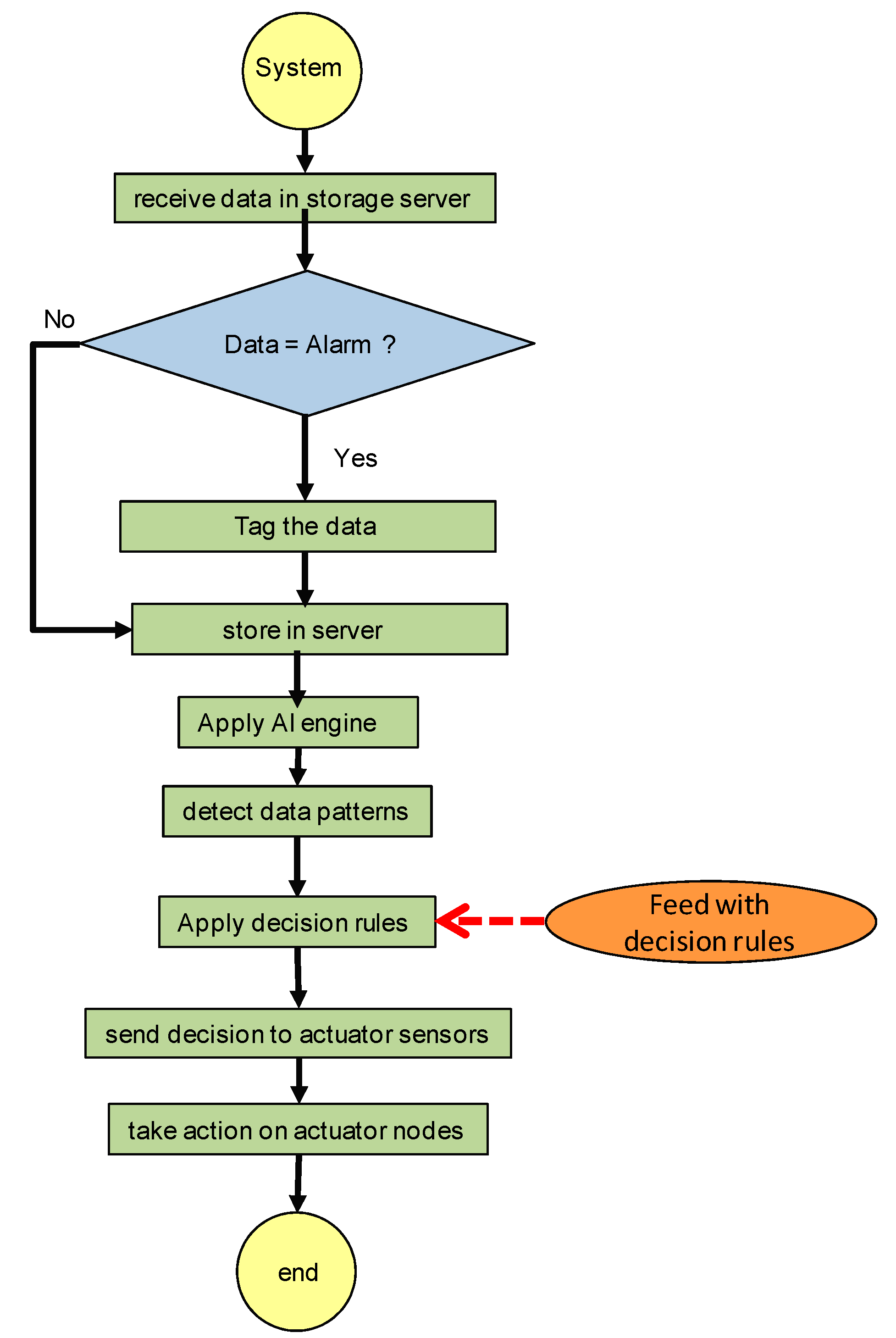
The second algorithm that we propose so as to store the data and alarms that are generated in the sensor nodes is provided in Figure 6. Once saved, they are processed by AI and then the decisions that are made are forwarded to the actuator nodes.

Initially, when the data are received in the Storage Server, the system must differentiate if it is an alarm or if it is the data that have been obtained during an observation period. In case of an alarm, the received data will be tagged before being stored. If it is not an alarm, the data are stored directly. Then, they go to the computer where they are treated by AI. In this way, patterns of behavior can be detected. Depending on the problems that can be detected and the place where actions should be applied, several decision rules have been created. Those rules are applied based on the detected patterns. Finally, the decisions that have been made based on the rules are sent to the actuator nodes so that they are put into action in an appropriate manner.

2.4. Protocol Description

In this subsection, the protocol utilized to make the proposed system work is presented.

Our proposed protocol, as can be seen in Figure 7, is divided into four fundamental phases, which are: Discovering Neighbors, Send Data, Storage and Data Processing, and Action. As its name suggests, in the Discovering Neighbors phase, the different sensor nodes send wireless signals to discover the nodes that are part of the group. Then, the sensor nodes determine the Central Node, and the Central Node identifies the gateway which is the Central Node in Urban Area 0. Therefore, a LoRa multi-hop network is established as in [15,16].

Once the nodes are activated and their connection is established, they go into the Send Data phase. The different sensors that are connected to each node begin to measure their respective parameters. The data collection period has been set to take place every minute. If the observed data differ by an amount greater than a previously established threshold, the measurement is sent to the Central Sensor Node of the group, and this node will store the data and compare them to check if they exceed the alarm threshold. It also checks if the alarm has been detected by more than one of the sensors of the group in order to provide fault tolerance capabilities. In case of exceeding the alarm threshold, the data are forwarded to the Central Sensor Node of Urban Area 0. Then, it is forwarded to the central storage system in the data center. In case of not exceeding the alarm threshold, the data are stored in the Central Sensor Node of the group until all the data are sent every 24 h period. Every day, the Central Sensor Node of Urban Area 0 will send all data to the Storage Server through the wired network.

The next phase is responsible for making the decisions to correct anomalies. It is the Data Processing phase. In this phase, the data are sent from the Storage Server to the AI system. This system will be responsible for making the pertinent decisions that will be sent to the actuators.

Finally, during the Action phase, the operation that the AI system considers adequate to solve the problem detected by the sensors will be sent to the Actuator Nodes.

2.5. Simulation Description

In this section, the considerations under which the simulation was conducted are detailed.

2.5.1. Water Details

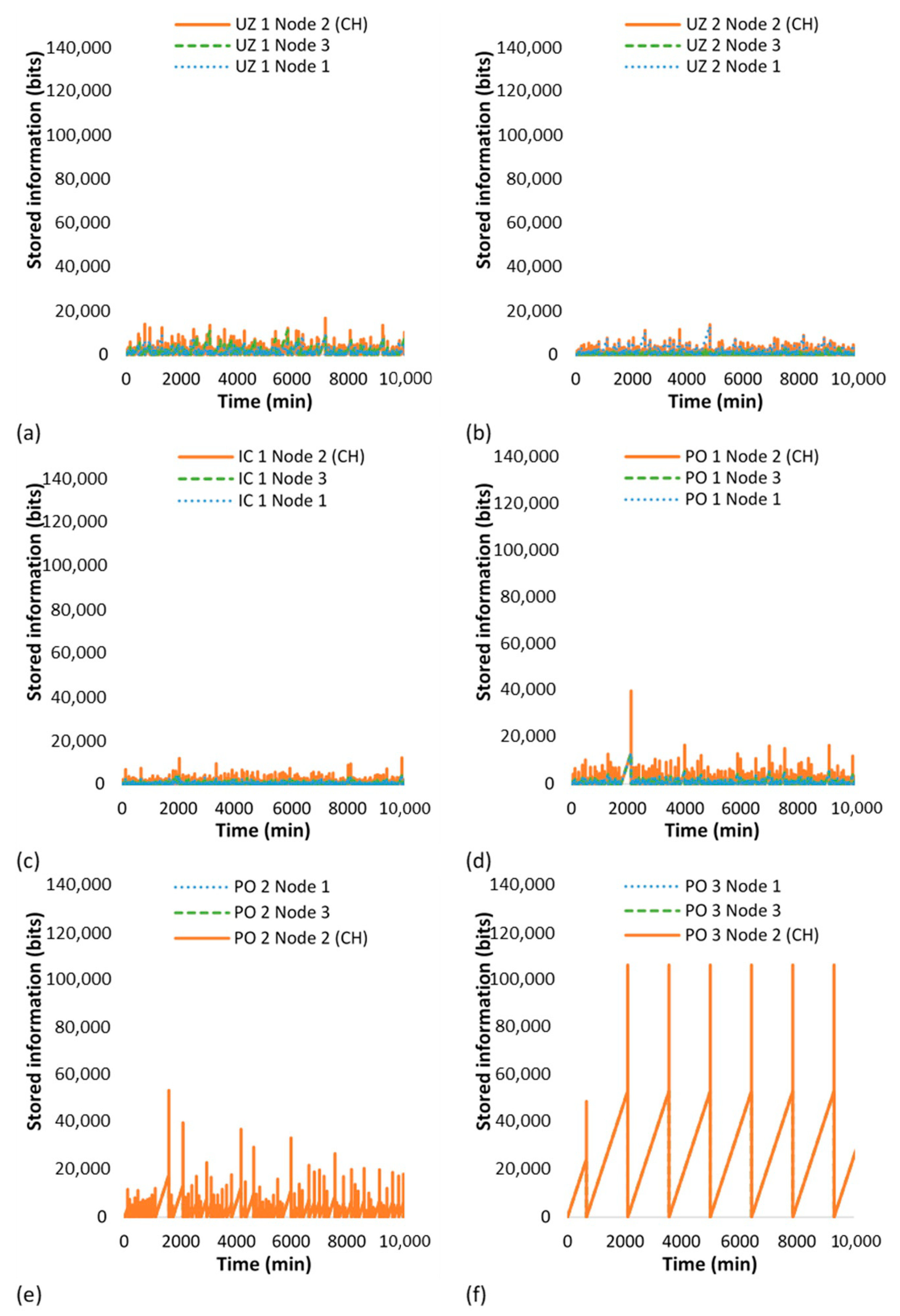
For the simulation, we have considered a region that entails two urban areas (UAs) with their channel to collect the water, the main channel, and one irrigation channel (IC) with the small pools (POs) in which water is treated. A total of 6 locations are considered in this simulation: 2 urban areas (UA1 and UA 2), the irrigation channel (IC 1), and the 3 pools (PO 1, PO 2, and PO 3.). In each one of these areas, a total of three nodes (a cluster) is located. The cluster comprises three nodes with LoRa interfaces. The six locations are close enough to ensure good coverage with a single LoRa gateway.

Since we are going to simulate our results using the algorithms described above, we need to generate different values of pollution in the monitored areas. To generate these values, we have included in our simulations the movement of water from point to point and some pollution inputs generated by random numbers at different intervals. The generated pollution coming from UAs and the pollution from the IC is diluted into the channel and flows to the next station. The pollution levels are maintained along with the IC. They only decrease in the pools where biosorption material is cleaning the water. Each pool has the capacity to reduce 50% of the pollution present in the water.

The following consideration is the probability of a false positive or a false negative due to an abnormal monitored value of one of the sensors. We have defined the chance of giving a false positive as 5% and 1% for a false negative.

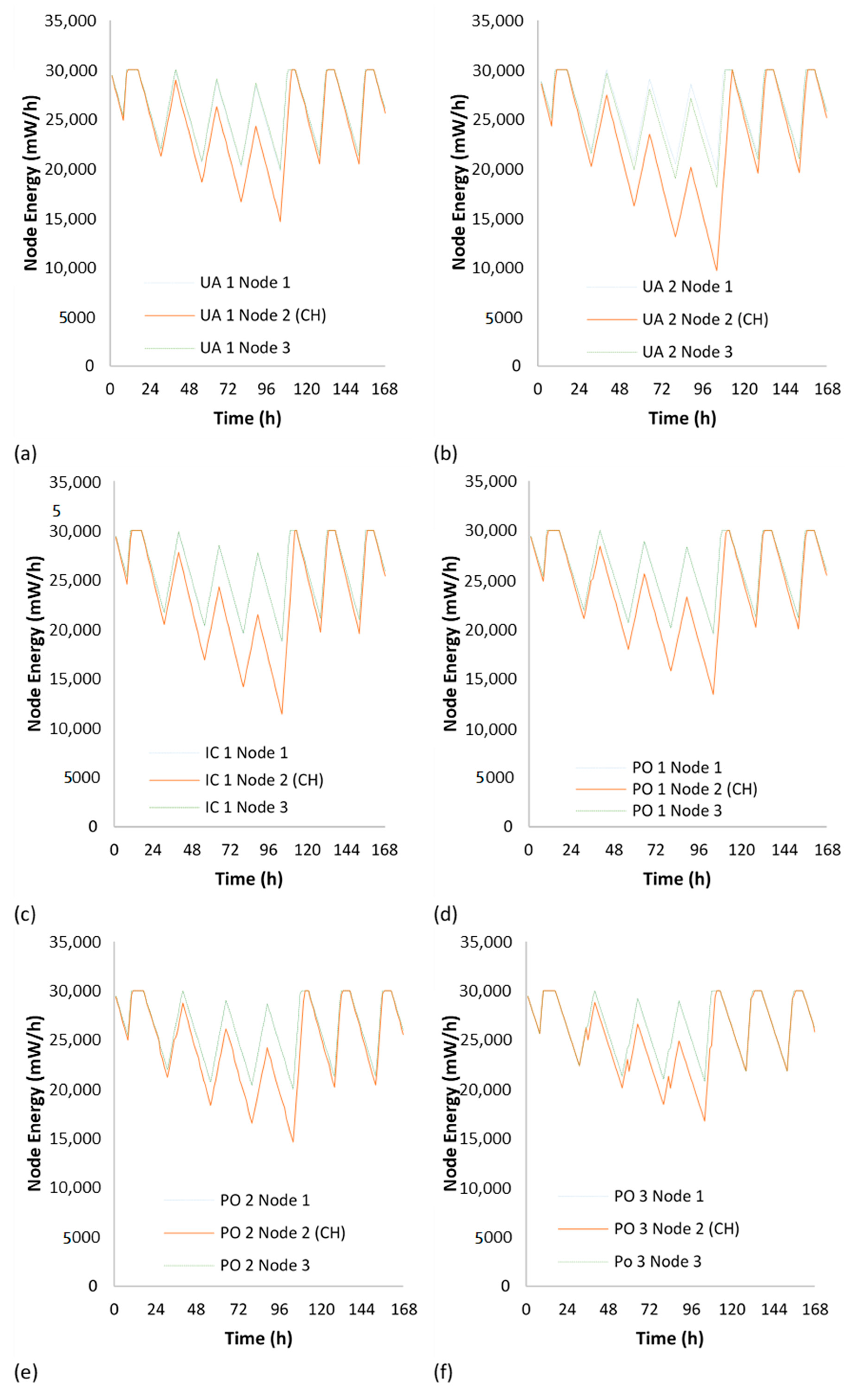
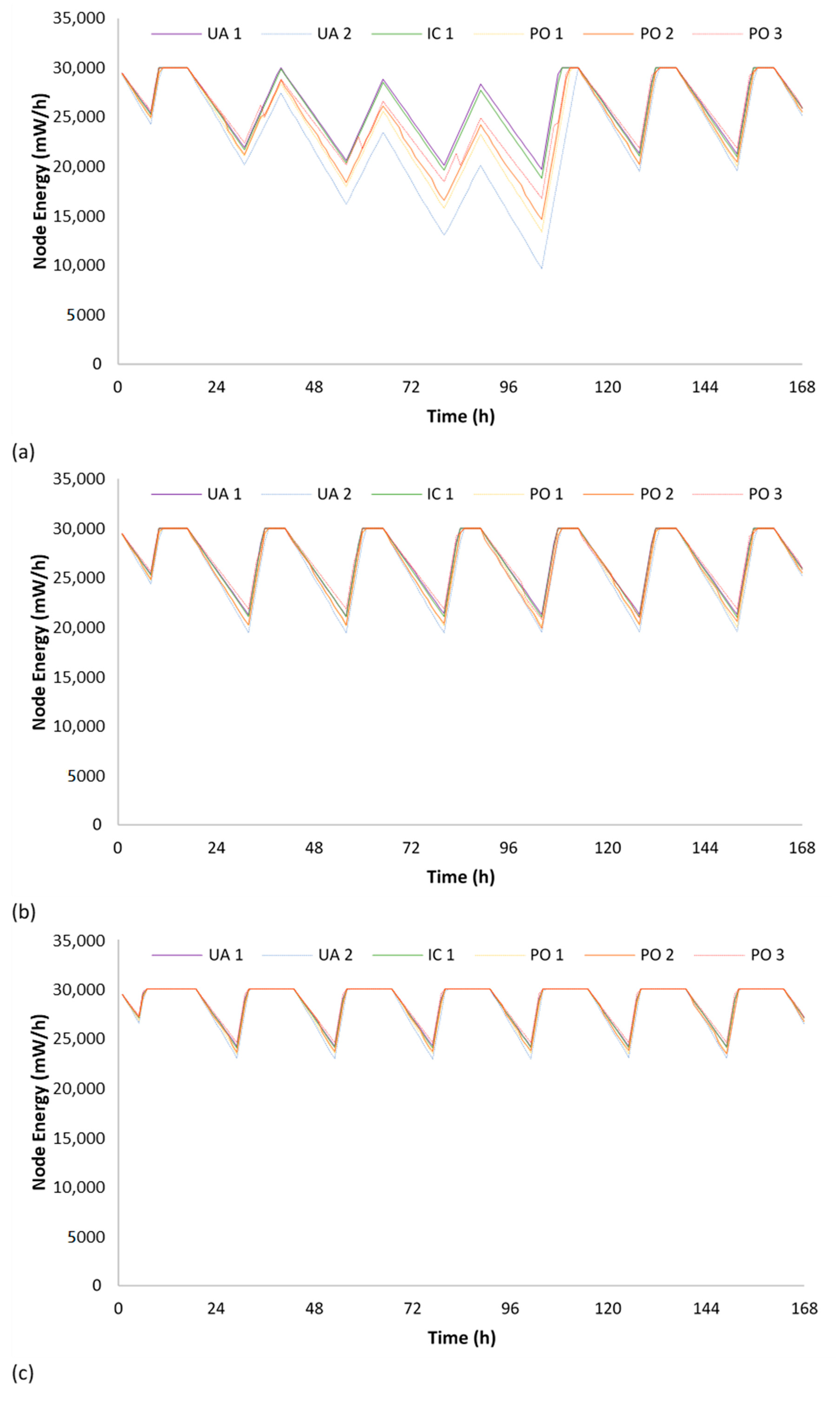
The simulation has a duration of one week in which each sensor measures the water quality once per minute. This timing is required since the arrival of pollution to the fields can transfer the problem of pollution from the water to the soil, and in this medium, the recovery is more complex. The simulation is carried out in two different periods of the year, in summer and in winter. This will affect only the energetic-related parameters.

2.5.2. Network Details

Regarding the packets sent through the network, we consider that the sensed data have a length of 37 bits for each measurement. The headers of the packets sent through LoRa comprise a preamble of 8 bytes and a header of 13 bytes. The data packets that are forwarded over LoRa will have a minimum size of 141 bits, which corresponds to a message with one measurement. Furthermore, the maximum packet size is 4176 bits, which is the maximum size allowed by LoRa. Lastly, the LoRa acknowledgements (ACK) have a size of 21 bytes which corresponds to the preamble and the header.

The simulation for the energy consumption of the LoRaWAN nodes is performed according to the energy consumption model presented in [17]. The total energy consumption of the node is presented in Equation (1).

E_Total = E_{Microcontroller} + E_Sensors + E_tx + E_rx

(1)

where E_{Microcontroller} is the energy consumed by the microcontroller, E_Sensors is the energy consumed to activate the sensors and gather the data, E_tx is the energy consumed to transmit the data, and E_rx is the energy consumed to receive the ACK from the gateway, which according to [17] is 0.27 mJ.

Equation (2) is utilized to determine the energy consumption per bit at the transmission.

E_bit = (Power Consumption x ToA)/(8 x (Preamble + Header + Payload))

(2)

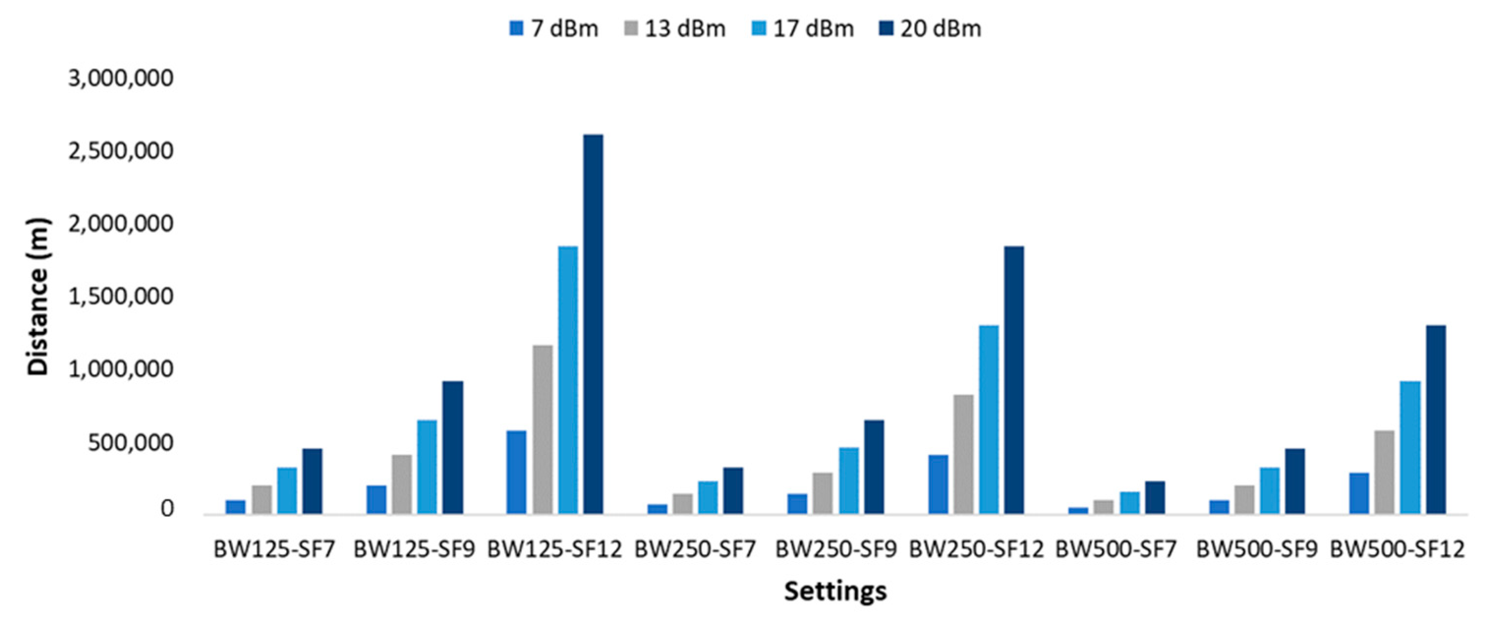
As for the LoRaWAN parameters, considering that our system requires a minimum range of 2 km, all possible settings would meet the requirement in the scenario of free space for a frequency of 868 MHz (See Figure 8). However, as there are vegetation and trees in the area, we consider a scenario with few obstacles, as presented in Figure 9. Therefore, for a transmission power of 7 dBm, the settings of BW250-SF7 and BW500-SF7 would not meet the requirement. For the case of 433 MHz, the required maximum theoretical distance is reached with all settings.

Considering the results of the theoretical distances for each LoRa setting, the settings selected for our system are the EU 863–870 frequency band, BW 125 kHz, and SF 8. Therefore, for the selected settings and a selected transmission power of 13 dBm with its power consumption of 92.4 mW/h, the energy consumed per bit for each sensor is 45.55 μJ.

3. Results

In this section, we present the results of our simulation. First of all, the storing and sending procedure of each node is represented as the SD status. Then, the bandwidth of the full network is depicted. Finally, the issues related to the remaining energy in the node are evaluated.

3.1. Status of the SDs

Considering the protocol described in Figure 7, one of the main aspects of this protocol is storing data, instead of sending it, waiting until the moment in which the water quality changes to send all stored data. We have to consider that the nodes which are not a Cluster Head (CH) store the data before sending them to the CH once the node detects a change. This procedure implies that the CH node stores large amounts of data just before sending them. Figure 10 and Figure 11 show the stored information in the SD of each one of the included nodes in our topology. While Figure 10 focuses on the first 60 min of the simulation, allowing for seeing some of the processes in detail, Figure 11 summarizes the whole simulated period.

In Figure 10, we can identify the stored information in the SDs of the clusters of six included locations: (a) UA1, (b) UA2, (c) IC1, (d) PO1, (e) PO2, and (f) PO 3. Focusing on Figure 10a, we can identify that the three nodes store information until minute 35. In minute 35, Node 3 and Node 2 detect a change in water quality. Node 1 has a false negative. Node 3 sends data to Node 2 and erases the data. Then, Node 2 checks that both nodes registered a change and sends all the data stored in the SD to the gateway. We can identify that Node 3 continues storing information during the rest of the period. In UA2, in Figure 10b, we can see the same case in minute 5, in this case, Node 3. Then, we identify a case in which the three sensors detect a water pollution change, see minute 52. In that case, the two nodes (Node 1 and Node 3) send the CH node data. Thus, the stored information is incremented three times. At that moment, the SD of the CH node stored 5550 bits of information. Similar cases can be seen in Figure 10c in minutes 41, 47, 51, and 59, and in Figure 10d in minutes 51 and 57. This delay of 10 min between IC1 and PO1 is the simulated time that the water remains in each pool. Finally, Figure 10e,f show the normal data storage process in the SDs. Since water is treated twice and three times, there are fewer water quality changes.

On the other hand, Figure 11 shows the SD usage for each node along the simulated period of one week. We can identify that locations UA1, UA2, and IC1 have a similar trend. All these areas, in Figure 11a–c, have low volumes of data stored in the SDs due to the constant exchange of information with the gateway caused by changes in water quality. Meanwhile, PO1, PO2, and PO3 are clusters characterized by larger amounts of data stored in the SDs, particularly during the second day of our simulation. In general terms, we can see that areas characterized by a lot of change follow the patterns seen in Figure 10. We can have false positives, false negatives, or true positives related to the water quality, which induce the sending event of stored data. In addition, we can see a secondary pattern here, mainly in the areas characterized by a lower degree of change. In these cases, when no changes are detected, Node 1 and Node 3 send all the information to the CH at midday to free their SDs, and as a method of control, as explained in Figure 5. This behavior can be particularly identified in the node of PO3, in which the unique movements of data in the SDs are related to the process. Thus, we identify a pattern of storing information until midday when all the data are sent to Node 2, and then Node 2 sends data to the gateway to free its SD. The maximum amount of stored information is 106,486 bits (13.3 Kbytes).

3.2. Consumed Energy

Figure 12 and Figure 13 show the node energy. The nodes have an energy harvesting system that has been dimensioned to ensure that it can cover the node’s energy requirements. In comparison, Figure 12 shows the remaining energy along with the simulation in each location in the worst scenario (winter with three consecutive days with a reduced energy harvesting). We can see the different locations in Figure 12a–f. In all four locations, we identify a similar trend. Node 2 is the node that consumes more energy since it receives the information of Nodes 1 and 3 and sends all the information to the gateway. Nodes 1 and 3 of each location have the same tendency in their energy levels in general terms. No significant differences can be seen among the energy levels of Nodes 1 and 3, along with the locations. Nonetheless, the energy of CHs differs from one location to another.

The CHs of locations with greater changes in water quality (Figure 12a–c) send more packets which are translated into more energy consumption. The CH with higher energy consumption is the CH of UA2 (Figure 12b). This node reaches a minimum energy of 12,320 mW/h just before the sunrise of the fifth day. The rest of the CHs, located in areas with fewer or no changes in water quality (Figure 12d–f) have higher energy levels. Another interesting trend can be identified in PO3 (Figure 12f). We can see a sharp decrease in energy levels at midday due to the large amounts of data sent at that moment. The absence of water quality conditions causes this during the rest of the day. Since the other CHs send data when the nodes detect a change, this decrement of energy level is distributed throughout the day.

Finally, Figure 13 shows the energy level of CHs in three different simulations for which we have modified the energy harvesting conditions. Figure 13a represents the worst conditions, the winter period with just 9 h of energy harvesting and three consecutive days with a reduction of 50% in the energy harvesting. These results summarize the data shown in Figure 12. Figure 13b shows a period of winter but without attenuated energy harvesting. We can identify that the CH of UA2 still has lower levels of energy than the others. Nevertheless, the difference is lower than in the previous scenario. On the other hand, Figure 13c shows a period of summer without attenuated energy harvesting. In this case, we have 14 h of energy production. We can see that the energy levels of CHs are similar to those in previous cases. During summer, nodes have their batteries full for most of the day.

3.3. Consumed Bandwidth

Figure 14 portrays the entire network’s consumed bandwidth, including the communication inside each cluster and the communication between the CHs and the gateway. A detail of the consumed bandwidth of a short period can be seen in Figure 14a. It represents the first 720 min of the simulated network, the first half of the day. We can see that in a considerable amount of time, the network does not generate any packet exchange due to the application of the algorithm described in Figure 5. In this simulation, during the first 720 min, we can identify that in 612 min, there is no exchange of information in our network. Minute 661 is the moment when all the information is sent to the gateway. At this moment, we reach the maximum bandwidth usage, 177,187 bits/min (2.95 kbps).

Considering Figure 14b, we can identify the consumed bandwidth during the whole simulated period. We can find seven peaks in the consumed bandwidth, which correspond to the seven middays. The maximum peak in this period is found on the second day. At that moment, a consumed bandwidth of 381,357 bits/min (6.35 kbps) can be identified. It is important to note that among the 40 performed simulations, we have represented the one with the highest maximum bandwidth. Figure 14c shows the box and whiskers diagram of the maximum bandwidth of all the 40 simulations. The average maximum bandwidth is 306,411 bits/min (5.1 kbps). With the selected LoRa settings, the maximum data rate is 3125 bps [18]. Therefore, we conclude that the data of the third cluster should be forwarded in two periods to avoid peaks of bandwidth consumption above 3125 bps.

A second simulation was performed to verify that changing the data forwarding settings of cluster three to two data forwarding times, being 9 h and 21 h, allows the bandwidth to remain below the maximum 3125 bps. The consumed bandwidth in the second simulation is presented in Figure 15. Figure 15a shows the results for a short period of time. In this case, the first 1400 min are shown as the system spends more than 1100 min with low bandwidth consumption. Then, there is a peak of 155,011 bits/min (2.58 kbps). The results for the complete simulated period are shown in Figure 15b. The peak with the highest bandwidth consumption is the same as the one displayed in Figure 15a. The second highest bandwidth consumption peak reached 142,764 bits/min (2.37 kbps).

Another 40 simulations were performed to obtain the box and whiskers diagram of the maximum bandwidth for this simulation scenario (See Figure 15c). The average maximum bandwidth was 128,204 bits/min (2.13 kbps). Furthermore, the change produced in the simulation does not have relevant repercussions on the global energy consumption of the proposed system.

4. Discussion

In this section, a discussion is given on the previous related works on protocols designed to be applied to WSNs that are employed in agricultural monitoring systems or to reduce the consumed energy for their functioning. Furthermore, the positioning of the water quality sensors and previous works on this topic are discussed as well.

WSNs have specific requirements and several protocols were developed specifically for these types of networks. Many systems for agricultural monitoring employ these protocols to forward the data obtained from the sensors. U. B. Nagesh et al. presented in [19] the usage of a message queuing telemetry transport (MQTT) protocol applied to precision farming and weather monitoring. The proposed system monitored humidity, temperature, and power and utilized a Raspberry Pi as the controller. The Eclipse Paho MQTT client was utilized to implement the subscriber and an open-source MQTT broker was utilized to access the data. A system for controlling and monitoring a smart greenhouse employing IoT and the MQTT protocol was presented by Dipen J. Vyas et al. in [20]. The system comprised an ESP8266 Wi-Fi module and an Atmega328 board with temperature, humidity, and soil moisture sensors. For the MQTT broker, the authors utilized Mosquitto. Ravi Kisore Kodali et al. introduced in [21] a low-cost smart irrigation system that employed MQTT as the communication protocol. The system comprised the ESP8266 NodeMCU-12E, a soil moisture sensor, a temperature and humidity sensor, and a relay. Junsung Park et al. presented in [22] a greenhouse monitoring and control system. Communication among the nodes was performed over ZigBee employing the UDP-based CoAP communication protocol. Nodes sent the gathered information from the sensors to the gateway which converted the CoAP message into an HTTP one so as to forward the data to the server. Finally, A. Paventhan et al. performed in [23] a comparison of two different protocols for WSNs in agricultural environments. The authors compared a simple network management protocol (SNMP) and a constrained application protocol (CoAP) in its message format, security, and resource management, and the user interface. They concluded that the CoAP presented better integration with the web and was expected to grow in usage for WSN applications.

Other protocols were created so as to address specific requirements of precision agriculture. Awais Ahmed et al. presented in [24] a routing protocol for WSNs to improve energy efficiency in environmental monitoring deployments. The energy-efficient sensor network routing (EESNR) protocol reduced the overhead of control messages. All the nodes were able to become the cluster head as long as the constraint on energy life and the established criteria was met. The authors performed simulations in NS3, comparing the proposed protocol to other existing protocols for WSNs like LEACH and its variations. The results showed an improvement of 27.8% of the lifespan of the sensors compared to the other protocols. A routing protocol for sensor networks intended for agriculture monitoring based on the efficient zone was developed by Lutful Karim et al. in [25]. An energy-efficient zone-based routing protocol (EEZRP) assigned different zones to the nodes depending on their distance to the base station and considering that nodes closest to the base station consume more energy. The proposed protocol considered the sensing range. The number of active nodes was fewer than in other protocols, but it might perform more processing and control operations. Simulations were performed to compare the energy consumption of the nodes to other protocols intended for WSNs like LEACH and DSC. The results showed a significant reduction of the consumed energy compared to other protocols. S. Bhagyashree et al. proposed, in [26], Apteen, a protocol intended for expanding the lifetime of the nodes in WSNs for precision agriculture. It is a cluster-based hierarchical routing protocol that groups the nodes into clusters comprising a cluster head and member nodes. The sensed parameters, thresholds, time division multiple access (TDMA) schedules, and the count time were broadcast from the cluster head. The messages were forwarded utilizing ZigBee in order to send the data to a database. Karim Fathallah et al. presented, in [27], partition aware RPL (PA-RPL), a routing protocol for IoT in precision agriculture. It was a version of the routing protocol for LLN (RPL) protocol that considered the partitions in farmlands to perform the routing topology. The protocol only considered one sink node. Simulations were performed employing the Cooja simulator. The results showed that the protocol was able to construct the network covering all the parcels. Lastly, a MAC protocol for precision agriculture based on storage and delivery intended for air–ground collaborative wireless networks (SD-MAC) was introduced by Song-Yue Liew et al. in [28]. In their proposal, an unmanned aerial vehicle (UAV) flew over the sensors in order to collect the gathered data. This way, a reduction in the duplication of data was obtained and the cost was reduced as a single UAV was able to gather the data from a large area. The proposed protocol forwarded the packets only when the UAV was within the range of the sensor. Sensors were deployed outside of the range of other sensors so as to avoid interferences. When the UAV was not close to the sensor, the sensor stored the information until the UAV was within range. Simulations were performed, comparing the proposed protocol to ALOHA. The results showed that the proposed protocol outperformed ALOHA.

Regarding sensor networks for water quality monitoring and wastewater treatment, the contamination of the wastewater may not only affect the quality of the water but also the treatment plants or the sewer systems. Therefore, it is important to deploy a monitoring network to detect contamination and contain the affected areas. In their study, Mariacrocetta Sambito et al. [29] compared different sensor positioning techniques intended for nonconservative immanent pollutants. The results showed that the optimal solution could be reached with less computational effort by implementing pre-screening and gray information techniques. Stefania Piazza et al. utilized an optimization approach by using the NSGA-II algorithm to compare the positioning of the sensor probes to the results obtained from experimental tests [30]. The results showed that the sensors positioned at the center of the network minimize the redundancy and maximize the detection likelihood.

Our work has presented a new algorithm and protocol for the detection and treatment of waters that other authors have not previously defined. We have utilized LoRaWAN, a low-power wide area network (LPWAN) protocol that supports low-cost, mobile, and secure bi-directional communication for the Internet of Things (IoT), which allowed a high level of energy saving and transmission over distances of several kilometers. Therefore, the proposed system allows its implementation in areas where it is difficult to get electric power to keep the devices active. Our devices, due to their low consumption, can be powered by batteries that are recharged through solar panels.

5. Conclusions

Produce can be affected by the quality of the irrigation water and, therefore, affect the people that consume it. Therefore, monitoring water quality is important to ensure food safety. In this paper, we have proposed an architecture and communication protocol for an irrigation water quality monitoring system for precision agriculture. It is based on groups of sensor nodes that monitor the water quality of the main canal and of biosorption auxiliary canals to determine if the water needs to be treated. Simulations were performed to determine the amount of data stored on the SD card of the nodes, the consumed bandwidth, and the energy consumption of the system. The results show that the proposed system is able to transmit the necessary information and alerts with a low bandwidth generation. However, the scheduled data forwarding of the central node of the last auxiliary canal had to be modified to two transmissions instead of one to ensure the fair access policy of LoRa. Lastly, the system is able to sustain energy consumption even on winter days with fewer hours of light and adverse weather conditions. Therefore, when considering data transmissions for wireless networks using LoRa communications, the addition of data pre-processing techniques would be beneficial to reduce energy consumption and ensure that the fair access policy is not violated.

For future work, the proposed protocol will be adapted to include the monitoring of the field area and tests will be performed on different vegetated environments. Furthermore, data pre-processing techniques will be implemented to improve the performance of the system.