Abstract
Modern power systems are subject to waveform distortions that include spectral components (supraharmonics) in the range of 2–150 kHz. Due to the lack of regulation in this range and since supraharmonics may follow time-varying patterns, the operators can take advantage of the statistical characterization of supraharmonics, e.g., for determining convenient power quality limits or to analyze the residual capacity of networks toward further installations of power electronic converters. This paper studies the statistical characterization of supraharmonics in low-voltage distribution networks, considering both the overall supraharmonic distortion (through the characterization of the total supraharmonic distortion index) and individual supraharmonic components. Several probability distributions are proposed and compared, also considering multimodal distributions that can fit more general scenarios in which the supraharmonic emissions follow regime patterns. The outcome of numerical experiments based on publicly available data collected at actual low-voltage distribution networks suggests that multimodal distributions are useful in characterizing supraharmonics in most cases, with acceptable goodness of fitting even in the presence of stair-shaped empirical distributions. This paper can serve as a starting point for the development of probabilistic power system analysis tools accounting for supraharmonic emissions and for the convergence toward standardization in the 2–150 kHz range.
1. Introduction
Power systems are undergoing a smart transition toward more sustainability and efficiency. This process passes through the widespread installation of distributed generation (e.g., renewables and small-scale generators), energy storage systems (fixed installations or mobile installations, such as electric vehicles), and high-efficiency loads [1,2,3]. These devices are typically interfaced to low-voltage distribution networks through electronic converters that introduce disturbances into voltage and current waveforms. The recent development of high-performance control systems determines emissions of spectral components that are beyond the classical 2 kHz milestone that individuates the low-frequency components, as they can reach up to 150 kHz for the common switching frequencies of the converters. The components in the range 2–150 kHz, typically labeled as supraharmonics in the relevant literature, have been studied much less than their low-frequency counterparts [4,5].
This topic remains challenging since supraharmonics, especially in the context of modern smart grids [6] and modern household devices [7], may be responsible for severe malfunctioning and loss of efficiency [8]. They may: (i) bring disturbances affecting the performance of control systems or the measurements taken by smart meters, (ii) interfere with communication networks, (iii) add thermal stress to devices and equipment, reducing their useful life [9,10]. Importantly, supraharmonics are not fully regulated yet [4,11,12], although in the very next years, they are expected to undergo specific regulations that will fix limits on the quality of the power supplied to the customers, as it is already common in the low-frequency range. Fixing these limits is still an ongoing process under discussion among regulators.
Considering that supraharmonics are typically time-varying, the efficacy of steady-state analysis to evaluate their impact on distribution networks is very limited. To cope with the time variation, the IEC 61000-4-30 standard [12] suggests considering the minimum, average, and peak values of the rms voltage during each aggregation interval in order to determine, e.g., typical emissions (through the average values) or worst-case emissions (through the peak values). However, relying on point minimum, average and maximum values is far from being exhaustive [11] since a complete characterization of the supraharmonic emissions is preferable.
Probabilistic harmonic analysis in the range 2–150 kHz may help in creating and studying scenarios to enable, e.g., taking precise actions for the most impactful components, determining the remaining available capacity of the network in terms of sustainable supraharmonic emissions (e.g., due to photovoltaics [13]), or compensation (e.g., through summing effect [14,15]). In addition, since supraharmonics are detected from source as primary or secondary emissions [16], the statistical characterization may be helpful to individuate and characterize these two hidden regimes. The statistical characterization of supraharmonics is handy in any of these frameworks, but it is still unexplored (it is worth noting that the statistical characterization of the low-frequency harmonics has been extensively treated instead [17,18,19]).
Related research on the statistical analysis of supraharmonics is in [11,20,21]. In [11,20], the empirical distributions of the supraharmonic emissions in low-voltage distribution networks are evaluated, although without including characterization aspects. The correlation between voltage and currents grouped components is evaluated using a time series approach in [21].
This paper contributes to the state-of-the-art statistical characterization of supraharmonics in low-voltage distribution networks. The topic is tackled at a global level (i.e., characterizing the overall emissions in the entire supraharmonic range) and at an individual-component level (i.e., characterizing the magnitude of individual supraharmonic components). Several probabilistic distributions are considered for the characterization, and they are compared in order to determine their performance in terms of goodness of fitting (GOF). Data collected at actual low-voltage distribution networks and publicly available at the PQube Live World Map database [22] are considered in the numerical experiments to foster the reproducibility of the results and future contributions to this topic.
In summary, the major contributions of this paper to the knowledge are:
- -
- This is one of the very few contributions on the statistical characterization of supraharmonics, setting a starting point for the development of probabilistic power system analysis tools accounting for supraharmonic emissions and for the convergence toward standardization in the 2–150 kHz range;
- -
- Several distributions are selected and compared to characterize both the overall supraharmonic emissions and the individual supraharmonic components;
- -
- The presentation of numerical experiments based on publicly available datasets that include supraharmonic data collected at multiple actual low-voltage distribution networks.
This paper is organized as follows. The methods for the statistical characterizations of supraharmonics are shown in Section 2; these include the techniques for the evaluation of the components from the measured waveforms, the definition of the power quality index that accounts for the global overall supraharmonic emissions, the distributions considered to characterize the supraharmonics and the GOF tests. Section 3 presents the results of the extensive numerical experiments based on actual public data. A discussion of the results and the conclusions are in Section 4.
2. Materials and Methods
The statistical characterization of supraharmonics performed in this paper aims at investigating the probability distributions that can effectively model the level of emissions in the range 2–150 kHz within an actual low-voltage distribution network. The statistical characterization can be useful for regulation purposes (e.g., to define thresholds as acceptable limits) and to predict the impact of the further installation of power electronic converters within a studied network by simulating scenarios. In addition, since supraharmonics are detected from source as primary or secondary emissions [16], the statistical characterization may be helpful to individuate and characterize the two hidden regimes.
This section discusses two approaches for the statistical characterization of the supraharmonics that are either based on the overall emissions within the entire 2–150 kHz range or on the single components at a given frequency band. A brief recall of the supraharmonic evaluation methods considered in the IEC 61000-4-30 standard [12] is presented as it is used to assess the individual components, and the total supraharmonic distortion (TSHD) index is introduced to provide the overall evaluation of the emissions within the entire 2–150 kHz range. Then, the probability distributions selected for the two approaches, the corresponding parameter estimation problems, and the methods to evaluate the GOF are described.
2.1. Supraharmonic Evaluation
The IEC 61000-4-30 standard [12] suggests three methods for the supraharmonic evaluation: (i) the CISPR 16-1-2 method [23], which is typically difficult to be applied by in-situ measurement systems; (ii) the extension of the grouping methodology, presented in the IEC 61000-4-7 for the frequency range 2–9 kHz, to the entire 2–150 kHz supraharmonic range; (iii) a method specifically presented in the standard [12], which considers measurements taken through cascaded high-pass and low-pass filters processed by a Discrete Fourier Transform (DFT).
The third method is recalled hereinafter, as it is the method considered by the in-situ measurement systems that provide the data for the numerical experiments [24].
The signal passes through cascaded high-pass and low-pass filters having proper poles to damp low-frequency components. A sliding window with an assigned width (multiple of the fundamental period, typically 10 cycles in 50-Hz power systems and 12 cycles in 60-Hz power systems) is applied to the filtered signal to obtain equally-spaced measurement sets, determining the analysis intervals. Each measurement set consists of discrete points that are processed through the DFT as:
where is the th sample of the signal, , and with as the sampling time. With proper settings, this is sufficient to estimate supraharmonic emissions and also to obtain some statistics upon them. For example, if and s, the DFT spectrum has a frequency resolution kHz, and 256 frequency bins can be evaluated; the first seventy-five of these bins include the entirety of the supraharmonic range. Since analysis intervals are considered, spectra can be estimated. The minimum, average, and peak values of the spectral components across the spectra can be calculated and recorded for statistical assessment purposes.
2.2. TSHD Index
The supraharmonic components evaluated through the methodology presented above can be characterized individually (i.e., considering the emissions related to a given band of frequency) or globally (i.e., considering an index that overall evaluates the emissions within the entire supraharmonic range 2–150 kHz). In this paper, the TSHD is the index that provides an overall evaluation of the emissions in the supraharmonic range.
The TSHD is defined as an extension of the total harmonic distortion (THD) for the supraharmonic range. Given the set of components in the supraharmonic range, the TSHD is defined as [11,25]:
where is the rated (fundamental) frequency of the power system.
2.3. Probability Distributions for the Statistical Characterization of Supraharmonics
The supraharmonics are assessed in this paper through two approaches. The first approach is a comprehensive one in which the TSHD is characterized through a considered probability distribution. The second approach is instead developed to characterize a single component within the supraharmonic range in order to suit the needs of the operator that focus on a specific frequency band for filtering, compensation, or capacity assessment purposes. In both approaches, the random variable object of the characterization is indicated with , which may stand for the TSHD (first approach) or for the th component (second approach).
The probability distributions considered for the characterization are briefly recalled below, with details on the maximum likelihood estimation (MLE) procedure used to estimate their parameters [26]. MLE makes statistical inference on a given dataset of observed samples in order to determine the estimates of the parameters of a distribution that maximize the probability of the observed data. Assuming that the generic distribution has probability distribution function (PDF) , where is the parameter vector, the likelihood function is defined for a given dataset of observed samples as the product of probabilities for the sample data :
The likelihood function depends only on the parameters of the distribution and, under the MLE approach, it is maximized to find the estimates of parameters . The generic optimization problem to be solved is:
Most of the distributions considered in this paper are unimodal, but due to the particularity of the supraharmonics (which can be time-varying and can have different source regimes), also a multimodal distribution, i.e., the mixture of normal distributions, is analyzed in this paper.
2.3.1. Normal Distribution
The normal (Norm) distribution is introduced as a benchmark for the statistical characterization due to its interpretability and since it assumes a regular and symmetric behavior of the random variable. The PDF is:
where , is the mean (i.e., a location parameter) and is the standard deviation (i.e., a scale parameter). The MLE of the parameters on a dataset of observed samples is:
2.3.2. Lognormal Distribution
For the analyzed phenomena, either the TSHD or individual supraharmonics can be zero or positive values; then, it is appropriate to include distributions having positive-real-valued support. The lognormal (LogN) distribution is among them, and it assumes that the logarithm of the random variable is normally distributed. The PDF is:
where is the mean of the logarithm of the random variable (i.e., a location parameter) and is the standard deviation of the random variable (i.e., a scale parameter). The MLE of the parameters on a dataset of observed samples is:
2.3.3. Weibull Distribution
The PDF of the Weibull (Weib) distribution is:
where , is a scale parameter and is a shape parameter. The MLE of the parameters on a dataset of observed samples has no explicit formulation, thus the implicit optimization problem (to be solved numerically) is reported:
2.3.4. Burr Distribution
The Burr distribution includes multiple distribution subfamily types and can fit a wider range of sampled data. It has three parameters, and its PDF is:
where , is a scale parameter and are shape parameters. The MLE of the parameters on a dataset of observed samples has no explicit formulation; thus, the implicit optimization problem (to be solved numerically) is reported:
2.3.5. Mixture of Normal Distributions
The mixture of normal distributions (MixN) is considered in this paper for the statistical characterization of supraharmonics due to its ability to model a multimodal behavior of the random variable. This may occur at low-voltage nodes that are subject to primary and secondary emission and/or to different operation regimes.
The -component MixN PDF is:
where , are the mean of the mixture components, are the standard deviations of the mixture components, and are the weights assigned to each component that satisfy:
The MLE of the parameters on a dataset of observed samples has no explicit formulation; thus, the implicit optimization problem (to be solved numerically) is reported:
Note that the MLE of the MixN parameters is complicated by the fact that the transition to the log-likelihood has no positive impact since the PDF is a weighted sum of exponentials in . Therefore, in this paper, we apply the expectation-maximization algorithm [27,28] to obtain the estimations of the parameters. Note eventually that is a hyper-parameter of the distribution; for the supraharmonic data considered in this paper, good characterization performance is achieved by picking between and .
2.4. GOF Evaluation: Adjusted Determination Coefficient and Q-Q Plots
The adjusted determination coefficient (ADC) is calculated to quantitatively assess the GOF of each distribution [28,29,30], and it is the metric used to select the most appropriate distribution for each data sample.
The ADC is defined from the determination coefficient (DC); if the domain of the random variable is divided in bins for GOF assessment purposes, the DC is:
where is the theoretical cumulative probability (calculated from the estimated distribution) of the random variable to belong to the th bin , is the number of data samples that are observed and lie in the th bin , and:
The ADC is introduced to calibrate the DC by the number of parameters involved in the estimated distributions, as more parameters typically tend to better capture the shape of the empirical data in characterization purposes but may be less useful out-of-sample as they tend to overfit the data. The ADC is defined as:
where is the number of parameters of the distribution.
The DC and ADC maximum value is 1; the closer they are to 1, the better is the fit. In this paper, the ADC is considered for GOF purposes in order to discern also by the number of parameters involved in the distribution.
The quantile-quantile (Q-Q) plots are further used for a graphical interpretation of the GOF. Q-Q plots illustrate the empirical data quantiles versus the theoretical quantiles determined by the estimated distribution. Q-Q plots that resemble a straight line (i.e., the bisector of the first quadrant) are more prone to identify an acceptable GOF.
3. Results
The statistical characterization of supraharmonics in low-voltage networks is performed considering actual data available from the PQube Live World Map of Power Quality [22]. The overall supraharmonic emission (through the TSHD) and individual supraharmonic components are characterized at several local locations across the world and through several weeks. Many case studies and scenarios have been developed; several of them are presented in this section.
3.1. Data Description: PQube Live World Map of Power Quality
The PQube Live World Map of Power Quality [22] is a publicly available database that includes data and variables of many PQ events across the world. The database is maintained by a manufacturer of PQ measurement systems, with the support and availability of facilities and academic institutions that host the measurement systems and distribute the data on the cloud platform.
For the purpose of this paper, the voltage data coming from PQube3 measurement systems are picked; these systems are indeed the ones able to monitor supraharmonics according to the IEC 61000-4-30 standard in the considered PQube database; therefore, the analysis reported below considers only locations at which a PQube3 measurement system is installed. To provide diversity, four locations—Austin (TX), Delray Beach (FL), Murphys (CA), Alameda (CA)—are selected from the USA, and four locations—Wohlen (Switzerland), Rochford (UK), Amsterdam (The Netherlands), Skelleftea (Sweden)—are selected from Europe.
The supraharmonic data is collected at each location for 14 days at a 1-minute time resolution. The data is directly provided by the form of voltage supraharmonic components grouped at 2 kHz; thus, 75 individual components are available. For each voltage supraharmonic component, the average (avg) and the peak value are provided for each minute, according to the specifications of the IEC 61000-4-30 standard. The case studies presented below will include both the avg and the peak data, either through the TSHDavg and TSHDpeak or the individual avg and peak components. Note that for the Austin and the Delray Beach dataset, only the avg components are provided.
3.2. TSHD Characterization
The TSHDavg and TSHDpeak evaluated at the eight locations are characterized through the Norm, LogN, Weib, Burr, and MixN distributions.
As an example of the obtained results, the estimated cumulative distribution functions (CDFs) of the TSHDavg and TSHDpeak for two locations (Alameda and Wohlen) are illustrated in Figure 1. The empirical CDF shapes of the TSHD data at Alameda clearly demonstrate the presence of regimes, which can be adequately modeled only through the multimodal MixN distribution. Particularly, the TSHDavg is captured only through a MixN with components. This behavior, however, is not generalizable, as, for example, the TSHDpeak at Wohlen has a cleaner behavior which can also be captured by the unimodal distributions.
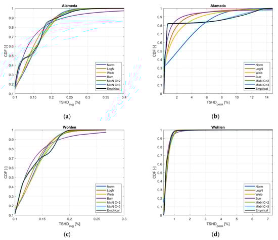
Figure 1.
Estimated and empirical CDFs of the: (a) TSHDavg at Alameda (CA); (b) TSHDpeak at Alameda (CA); (c) TSHDavg at Wohlen (Swizterland); (d) TSHDpeak at Wohlen (Swizterland).
The quantitative assessment of the GOF is reported in Table 1 through the ADC. Bold values indicate the best fit. The MixN distribution with components is always the best pick as it returns the greatest ADC in all the considered locations and scenarios.

Table 1.
Adjusted determination coefficient of the TSHD distributions. Bold values indicate the best fit.
In four case studies, the MixN with components has equal performance, denoting that a bimodal distribution is, however, effective when two regimes can be individuated. Restricting the analysis to the unimodal distributions, only the Burr distribution has overall the best characterization skill; in two case studies, i.e., TSHDpeak at Murphys and Wohlen, the Burr performs also better than the MixN with components. It is worth noting that the most common distributions, such as the Norm and the Weib, perform very poorly, especially in characterizing the TSHDpeak.
The Q-Q plot of the TSHDavg and TSHDpeak for Alameda and Wohlen is illustrated in Figure 2; for the sake of clarity, only the Burr distribution and the MixN distribution with components are considered in the Q-Q plots. The Q-Q plots of the MixN distribution with components are closer to resemble the bisector line, compared to the Q-Q plots of the Burr distribution, which cannot even be assimilated to a straight line. Only in the Alameda TSHDpeak case study, which is challenging as it is characterized by a pruned right tail of upper quantiles at high TSHD value, the Q-Q plot of the MixN distribution with components is less close to the ideal bisector line.
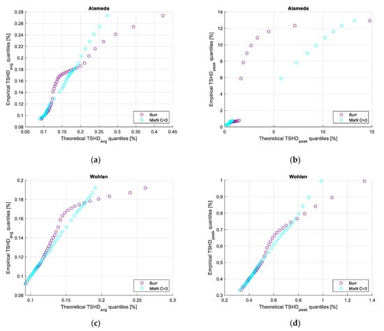
Figure 2.
Q-Q plots of the: (a) TSHDavg at Alameda (CA); (b) TSHDpeak at Alameda (CA); (c) TSHDavg at Wohlen (Swizterland); (d) TSHDpeak at Wohlen (Swizterland).
3.3. Individual Supraharmonic Component Characterization
The individual components evaluated at the eight locations are characterized through the Norm, LogN, Weib, Burr, and MixN distributions. Only for the sake of conciseness, the results presented below refer to four individual components (6, 26, 50, and 120 kHz) at Alameda; similar considerations arise from the analysis performed at the other locations. The 6-, 26-, 50-, and 120-kHz components are investigated as they are representative of the ranges 2–9, 9–30, 30–90, and 90–150 kHz, which are typically the object of interest in supraharmonic analysis [11]. Both the avg and the peak values are considered in the experiments.
The estimated CDFs of the four avg individual components and of the four peak individual components are illustrated in Figure 3 and Figure 4, respectively. The empirical CDF shapes of the avg individual components strongly differ from the empirical CDF shapes of the peak individual components: at a higher frequency, the CDFs of the avg components appear to follow a stepwise pattern, denoting regions of quasi-continuous avg supraharmonic emissions, whereas CDFs of the peak components appear to follow a continuous, slightly oscillating pattern, with distributed regions of peak supraharmonic emissions. The regimes identified for the peak individual components can be adequately modeled only through the multimodal MixN distribution. It appears instead that the benefit of applying the multimodal MixN distribution is reduced while considering the avg individual components at a higher frequency.
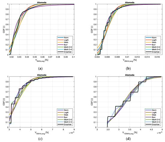
Figure 3.
Estimated and empirical CDFs of the: (a) 6-kHz; (b) 26-kHz; (c) 50-kHz; (d) 120-kHz avg voltage component at Alameda (CA).
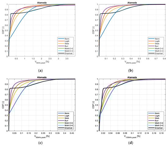
Figure 4.
Estimated and empirical CDFs of the: (a) 6-kHz; (b) 26-kHz; (c) 50-kHz; (d) 120-kHz peak voltage component at Alameda (CA).
The quantitative assessment of the GOF is reported in Table 2 through the ADC. Bold values indicate the best fit. The MixN distribution with components is the best pick in all the considered scenarios, as the ADC values are the greatest ones. As guessed by the graphical inspection, the use of a multimodal distribution has the most impact in characterizing the peak individual components as the unimodal components are particularly poor, whereas the gap between unimodal and multimodal distribution is more reduced in characterizing the avg individual components.
Table 2.
Adjusted determination coefficient of the individual component distributions at Alameda. Bold values indicate the best fit.
The Q-Q plot of the peak individual components at Alameda and Wohlen are illustrated in Figure 5; for the sake of clarity, only the Burr distribution and the MixN distribution with components are considered in the Q-Q plots. The Q-Q plots of the MixN distribution with components are closer to resemble the bisector line, compared to the Q-Q plots of the Burr distribution, which cannot even be assimilated to a straight line.
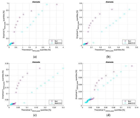
Figure 5.
Q-Q plots of the: (a) 6-kHz; (b) 26-kHz; (c) 50-kHz; (d) 120-kHz peak voltage component at Alameda (CA).
4. Discussion and Conclusions
The statistical characterization of supraharmonics is tackled in this paper to enable the generation of scenarios and to foster the probabilistic analysis of power systems accounting for emissions in the range 2–150 kHz. Several probability distribution families are considered to characterize supraharmonics within a detailed comparative scheme developed to generalize the approach and to suit different conditions and case studies. The numerical experiments performed on public data collected at actual low-voltage distribution networks confirm that the time-varying nature of supraharmonics is prone to be analyzed within a probabilistic framework; moreover, the characterization is conveniently optimized using multimodal distributions that are able to catch and model different operation regimes that determine a different entity of supraharmonic components. Among the considered distributions, the MixN shows the best fitting results in characterizing both the overall supraharmonic content (through the TSHD) and individual supraharmonic components. Notably, the estimated quantiles of the MixN maintain statistical consistency with the empirical data quantiles even at low and high nominal coverages, as confirmed by the Q-Q plot inspection at left and right tails.
Future research on this topic may follow several paths, such as the development of more appropriate probability distributions to model supraharmonics and the exploitation of the statistical characterization to generate scenarios and to implement probabilistic analysis with a specific focus on supraharmonic emissions (e.g., within probabilistic harmonic power flow studies). In perspective, this may also enable to take precise actions for the most impactful power system components, to determine the available remaining capacity of the network in terms of sustainable supraharmonic emissions, and to analyze the compensation (summing effects). The availability of wider datasets that are not burdened by the 2 kHz grouping may allow refining these procedures, accounting for a finer frequency resolution.
Author Contributions
Conceptualization, P.D.F. and P.V.; methodology, P.D.F. and P.V.; software, P.D.F. and P.V.; validation, P.D.F. and P.V.; formal analysis, P.D.F. and P.V.; investigation, P.D.F. and P.V.; data cu-ration, P.D.F. and P.V.; writing—original draft preparation, P.D.F. and P.V.; writing—review and editing, P.D.F. and P.V.; visualization, P.D.F. and P.V.; supervision, P.D.F. and P.V. All authors have read and agreed to the published version of the manuscript.
Funding
This research received no external funding.
Data Availability Statement
All the data used in the experiments reported in this paper are publicly available at the PQube World Live Map (http://map.pqube.com/).
Acknowledgments
The author is grateful to Marinica Guarino and Noemi Liguori for their contributions in gathering and pre-processing the data used in the numerical experiments.
Conflicts of Interest
The author declares no conflict of interest.
Abbreviations
| ADC | Adjusted determination coefficient |
| CDF | Cumulative distribution function |
| DC | Determination coefficient |
| DFT | Discrete fourier transform |
| GOF | Goodness of fitting |
| LogN | LogNormal distribution |
| MixN | Mixture of normal distributions |
| MLE | Maximum likelihood estimation |
| Norm | Normal distribution |
| Probability density function | |
| Q-Q | Quantile-Quantile |
| THD | Total harmonic distortion |
| TSHD | Total supraharmonic distortion |
| Weib | Weibull distribution |
| argmax | Argument of the maximum |
| avg | Average value |
References
- Sakar, S.; Rönnberg, S.; Bollen, M.H.J. Interferences in AC–DC LED Drivers Exposed to Voltage Disturbances in the Frequency Range 2–150 kHz. IEEE Trans. Power Electron. 2019, 34, 11171–11181. [Google Scholar] [CrossRef]
- Bollen, M.H.J.; Das, R.; Djokic, S.; Ciufo, P.; Meyer, J.; Rönnberg, S.K.; Zavodam, F. Power quality concerns in implementing smart distribution-grid applications. IEEE Trans. Smart Grid 2016, 8, 391–399. [Google Scholar] [CrossRef]
- Alfieri, L.; Bracale, A.; Varilone, P.; Leonowicz, Z.; Kostyla, P.; Sikorski, T.; Wasowski, M. Methods for assessment of supraharmonics in power systems. Part I: Theoretical issues. In Proceedings of the 2019 International Conference on Clean Electrical Power (ICCEP 2019), Otranto, Italy, 2–4 July 2019; pp. 110–115. [Google Scholar]
- Bollen, M.H.J.; Olofsson, M.; Larsson, A.; Rönnberg, S.; Lundmark, M. Standards for supraharmonics (2 to 150 kHz). IEEE Electromagn. Compat. Mag. 2014, 3, 114–119. [Google Scholar] [CrossRef]
- Mendes, T.M.; Duque, C.A.; Manso da Silva, L.R.; Ferreira, D.D.; Meyer, J.; Ribeiro, P.F. Comparative analysis of the measurement methods for the supraharmonic range. Int. J. Electr. Power Energy Syst. 2020, 118, 105801. [Google Scholar] [CrossRef]
- Yalcin, T.; Kostyla, P.; Leonowicz, Z. Supra-Harmonic Band Patterns in Smart Grid. In Proceedings of the 2020 IEEE International Conference on Environment and Electrical Engineering and 2020 IEEE Industrial and Commercial Power Systems Europe (EEEIC/I&CPS Europe 2020), Madrid, Spain, 9–12 June 2020; pp. 1–7. [Google Scholar]
- Espín-Delgado, A.; Busatto, T.; Ravindran, V.; Ronnberg, S.K.; Meyer, J. Evaluation of Supraharmonic Propagation in LV Networks Based on the Impedance Changes Created by Household Devices. In Proceedings of the 2020 IEEE PES Innovative Smart Grid Technologies Europe (ISGT-Europe 2020), Delft, The Netherlands, 26–28 October 2020; pp. 754–758. [Google Scholar]
- Espín-Delgado, A.; Rönnberg, S.; Letha, S.S.; Bollen, M. Diagnosis of supraharmonics-related problems based on the effects on electrical equipment. Electr. Power Syst. Res. 2021, 195, 107179. [Google Scholar] [CrossRef]
- Ronnberg, S.K.; Bollen, M.H.J.; Amaris, H.; Chang, G.W.; Gu, I.Y.H.; Kocewiak, Ł.H.; Meyer, J.; Olofsson, M.; Ribeiro, P.F.; Desmet, J. On waveform distortion in the frequency range of 2–150 kHz—Review and research challenges. Electr. Power Syst. Res. 2017, 150, 1–10. [Google Scholar] [CrossRef]
- Irish Standard Recommendation CLC/TR 50627:2015. Study Report on Electromagnetic Electromagnetic Interference between Electrical Equipment/Systems in the Frequency Range below 150 kHz. CENELEC: 2015. Available online: https://infostore.saiglobal.com/preview/98704574178.pdf?sku=879471_saig_nsai_nsai_2089711 (accessed on 15 April 2021).
- Rönnberg, S.K.; Gil-De-Castro, A.; Medina-Gracia, R. Supraharmonics in European and North American low-voltage networks. In Proceedings of the 2018 IEEE International Conference on Environment and Electrical Engineering and 2018 IEEE Industrial and Commercial Power Systems Europe (EEEIC/I&CPS Europe 2018), Palermo, Italy, 12–15 June 2018; pp. 1–6. [Google Scholar]
- IEC 61000-4-30 International Standard. Electromagnetic Compatibility (EMC)—Part 4-30: Testing and Measurement Techniques—Power Quality Measurement Methods. IEC: 2015. Available online: https://infostore.saiglobal.com/preview/is/en/2009/i.s.en61000-4-30-2009.pdf?sku=1118389 (accessed on 15 April 2021).
- Darmawardana, D.; Perera, S.; Robinson, D.; Meyer, J.; Jayatunga, U. Important Considerations in Development of PV Inverter Models for High Frequency Emission (Supraharmonic) Studies. In Proceedings of the 19th International Conference on Harmonics and Quality of Power (ICHQP 2020), Dubai, United Arab Emirates, 6–7 July 2020; pp. 1–6. [Google Scholar]
- Sultaria, J.; Delgado, A.E.; Ronnberg, S. Summation of Supraharmonics in Neutral for Three-Phase Four-Wire System. IEEE Open J Ind Appl. 2020, 1, 148–156. [Google Scholar] [CrossRef]
- Espín-Delgado, A.; Busatto, T.; Ravindran, V.; Ronnberg, S.K.; Meyer, J.; Bollen, M. Summation law for supraharmonic currents (2–150 kHz) in low-voltage installations. Electr. Power Syst. Res. 2020, 184, 106325. [Google Scholar] [CrossRef]
- Rönnberg, S.K.; Bollen, M. Measurements of primary and secondary emission in the supraharmonic frequency range, 2–150 kHz. In Proceedings of the CIRED International Conference and Exhibition on Electricity Distribution, Lyon, France, 15–18 June 2015. [Google Scholar]
- Langella, R.; Testa, A. Summation of Random Harmonic Currents. In Time-Varying Waveform Distortions in Power Systems; Wiley/IEEE: Chippenham, UK, 2009. [Google Scholar]
- Langella, R.; Testa, A. Probabilistic Modeling of Single High-Power Loads. In Time-Varying Waveform Distortions in Power Systems; Wiley/IEEE: Chippenham, UK, 2009. [Google Scholar]
- Baghzouz, Y.; Burch, R.F.; Capasso, A.; Cavallini, A.; Emanuel, A.E.; Halpin, M.; Verde, P. Time-varying harmonics. I. Characterizing measured data. IEEE Trans. Power Deliv. 1998, 13, 938–944. [Google Scholar] [CrossRef]
- Rönnberg, S.K.; Gil-De-Castro, A.; Delgado, E. Variations of supraharmonic emissions in low voltage networks. In Proceedings of the 25th CIRED International Conference on Electricity Distribution, Madrid, Spain, 3–6 June 2019; pp. 1–5. [Google Scholar]
- Novitskiy, A.; Westermann, D. Time series data analysis of measurements of supraharmonic distortion in LV and MV networks. In Proceedings of the 52nd International Universities Power Engineering Conference (UPEC 2017), Heraklion, Greece, 28–31 August 2017; pp. 1–6. [Google Scholar]
- PQube World Live Map. Available online: http://map.pqube.com/ (accessed on 21 February 2021).
- CISPR 16-1-2 International Standard. Specification for Radio Disturbance and Immunity Measuring Apparatus and Methods—Part 1-2: Radio Disturbance and Immunity Measuring Apparatus—Coupling Devices for Conducted Disturbance Measurements. CISPR: 2014. Available online: https://webstore.iec.ch/publication/31 (accessed on 1 February 2021).
- Powerside PQube 3® Application Note v.3.0. Conducted Emissions in the 2 kHz to 150 kHz Band Supra-Harmonics. Available online: https://help.powerside.com/knowledge/application-note-conducted-emissions-in-the-2khz-to-150khz-band-supra-harmonics-application-note (accessed on 21 February 2021).
- Zolett, B.; Leborgne, R.C. Propagation of Supraharmonics Generated by PMSG Wind Power Plants into Transmission Systems. In Proceedings of the 2020 IEEE PES Transmission & Distribution Conference and Exhibition—Latin America (T&D LA), Montevideo, Uruguay, 28 September–2 October 2020; pp. 1–6. [Google Scholar]
- Rossi, R.J. Mathematical Statistics: An Introduction to Likelihood Based Inference; John Wiley & Sons: New York, NY, USA, 2018. [Google Scholar]
- Bilmes, J.A. A gentle tutorial of the EM algorithm and its application to parameter estimation for Gaussian mixture and hidden Markov models. Int. Comput. Sci. Inst. 1998, 4, 126. [Google Scholar]
- Bracale, A.; Carpinelli, G.; De Falco, P. A new finite mixture distribution and its expectation-maximization procedure for extreme wind speed characterization. Renew. Energy 2017, 113, 1366–1377. [Google Scholar] [CrossRef]
- Draper, N.R.; Smith, H. Applied Regression Analysis, 1st ed.; John Wiley & Sons: New York, NY, USA, 1998. [Google Scholar]
- Carta, J.A.; Ramirez, P.; Velazquez, S. Influence of the level of fit of a density probability function to wind-speed data on the WECS mean power output estimation. Energy Convers. Manag. 2008, 49, 2647–2655. [Google Scholar] [CrossRef]
Publisher’s Note: MDPI stays neutral with regard to jurisdictional claims in published maps and institutional affiliations. |
© 2021 by the authors. Licensee MDPI, Basel, Switzerland. This article is an open access article distributed under the terms and conditions of the Creative Commons Attribution (CC BY) license (https://creativecommons.org/licenses/by/4.0/).