An All-Mach Number HLLC-Based Scheme for Multi-Phase Flow with Surface Tension

Abstract

This paper presents an all-Mach method for two-phase inviscid flow in the presence of surface tension. A modified version of the Hartens–Lax–van Leer Contact (HLLC) solver is developed and combined for the first time with a widely used volume-of-fluid (VoF) method: the compressive interface capturing scheme for arbitrary meshes (CICSAM). This novel combination yields a scheme with both HLLC shock capturing as well as accurate liquid–gas interface tracking characteristics. It is achieved by reconstructing non-conservative (primitive) variables in a consistent manner to yield both robustness and accuracy. Liquid–gas interface curvature is computed via height functions and the convolution method. We emphasize the use of VoF in the interest of interface accuracy when modelling surface tension effects. The method is validated using a range of test-cases available in the literature. The results show flow features that are in sensible agreement with previous experimental and numerical work. In particular, the use of the HLLC-VoF combination leads to a sharp volume fraction and energy field with improved accuracy.

1. Introduction

High-speed multi-phase compressible flow induced by blast or shock waves is of interest to both basic science and engineering [1,2,3,4,5,6,7,8]. For example, when a sample of a solid metal is subjected to a high-power laser beam, the large negative pressures created in the metal lead to its instant melting followed by micro-spalling [9]. In an underwater explosion, the detonation of an unconfined charge leads to the growth of a stable gas bubble [10]. In the design of liquid blast mitigants, the detonation of a confined explosive surrounded by a liquid layer leads to the jetting of finger-like structures or instabilities [11]. In these examples, the compressible effects, the liquid–gas interface motion and surface tension are key fluid physics phenomena [12,13].

Over the past three decades, efficient schemes for multi-phase compressible flow have been put forward. These may be broadly divided into three families of multi-phase modelling. First, the “two-phase” models where each phase is treated explicitly by its own set of equations. In this regard, the Baer and Nunziato [14] and Abgrall and Saurel [15] seven-equation models are popular [16,17,18]. The second approach reduces the two energy equations to a single one, which is equally valid. Examples include the reduced five-equation model of Kapila et al. [19] used in [1,20,21,22]. The third and final approach is a homogeneous flow model known as the “one-fluid” formulation, where an equilibrium is assumed to exist between the liquid and the gas phases. This one-fluid formulation has been extensively used in incompressible flow [23,24,25,26], and recently in compressible shock modelling [12,27,28] of liquid–gas systems. For this article, we shall consider the inviscid modelling of a liquid–gas flow via a homogeneous one-fluid method.

To capture the compressible characteristics in the flow, different solvers are outlined in the literature [1,12,20,27,28,29]. These comprise the popular Riemann- or Godunov-type schemes [29,30,31] and the semi-implicit projection solvers [32]. In this article, we shall employ the Hartens–Lax–van Leer Contact (HLLC) approximate Riemann solver [30] for its contact-preserving properties and its ability to maintain the positivity of variables. However, as will be demonstrated, when applied to track the liquid–gas interface, this solver results in smearing leading to the loss of liquid–gas interface resolution. Due to the latter, curvature cannot be computed accurately and hence surface tension is often not accounted for.

In recent years, different interface handling methods have been proposed to address this smearing. For instance, Daude et al. [20] extended the HLLC solver to an arbitrary Lagrangian–Eulerian (ALE) formulation to track the liquid–gas interface. However, their approach does not include any surface tension effects. Moreover, ALE methods are known to be limited by mesh distortions [33] and therefore require re-gridding procedures that are computationally expensive. Subsequent work on HLLC includes the use of a compression technique to remove numerical diffusion present at the interface. This approach was first proposed by Garrick et al. [1], where HLLC was re-formulated to allow for surface tension effects. However, their method does not take into account the liquid availability criteria [34] when advecting the interface. This is further discussed in the next paragraph.

The final class of interface-handling methods is that of the sharp interface techniques [35]. Notably, the volume-of-fluid (VoF) method is well-known [34,36,37,38] for its volume conservative properties. For example, Fuster et al. [12] successfully extended the unified semi-implicit compressible solver proposed by Xiao et al. [32] and combined their formulation with a geometric VoF method [36] to allow for the inclusion of surface tension effects. Here, the superior accuracy is due to accounting for liquid availability in mixed cells when computing phase fluxes. This ensures boundedness of the volume fraction field. However, historically, such VoF methods have been widely used for incompressible flow and have therefore mostly been used in conjunction with semi-implicit projection solvers [24,26,39,40].

Only recently has the use of VoF methods gained interest in the context of Riemann-type schemes [22,28]. For example, Shyue [27] is cited as the first to employ a geometric VoF method in conjunction with the Roe solver for a homogeneous two-phase flow without surface tension effects. Similarly, Corot et al. [28] combined a geometric VoF method with a newly derived Godunov scheme for surface tension but did not employ the HLLC solver. Jibben et al. [22] used a similar geometric VoF method with HLLC. However, in the latter cited work, conserved variables were reconstructed and the VoF method was restricted to Cartesian grids. Hence in this work, we propose the use of VoF and HLLC. As opposed to the cited work, we advocate primitive variable reconstruction in the interests of consistency and accuracy.

Extending earlier work, the Compressive Interface Capturing Scheme for Arbitrary Meshes (CICSAM) by Ubbink et al. [34] is employed to ensure conservative sharp interface tracking on arbitrary meshes. Second-order flux reconstruction of primitive variables ($\rho$, p and $\mathit{u}$) is ensured via the Monotone Upstream-centred Scheme for Conservation Laws (MUSCL) [41]. The use of this method ensures that shock waves are efficiently and accurately captured. Surface tension is accounted for via the continuum surface force (CSF) method where the interface curvature is reconstructed using the convolution method [4] on non-orthogonal meshes and height functions [2,3] on Cartesian grids. The implementation of the developed algorithm is done in the Elemental^®  [24,39,42,43] multi-physics platform. The developed solver is rigorously assessed via application to a range of benchmark test-cases from 1-D to 2-D.

2. Mathematical Formulation

2.1. Governing Equations

Inviscid immiscible compressible two-phase flow is considered where the governing equations are based on that by Abgrall and Saurel [15]. Here, a one-fluid formulation is derived from their work by defining a cell-average density $\rho$, pressure p and a uniform velocity $\mathit{u}$. In the absence of gravitational, viscous effects and heat conduction or phase change, these read in compact form as

$$\frac{\partial \mathit{U}}{\partial t}+\nabla ·\mathit{F}\left(\mathit{U}\right)=\mathit{S},$$

(1)

where $\mathit{U}={\left[\begin{array}{c}\rho ,\rho \mathit{u},\rho E,\alpha \end{array}\right]}^T$ is the set of conserved variables, $\mathit{F}$ and $\mathit{S}$ are the flve Study of Computational Mve Study of Computational M, as

$$\mathit{F}\left(\mathit{U}\right)=\left[\begin{array}{c}\rho \mathit{u}\\ \rho \mathit{u}\otimes \mathit{u}+p\mathit{I}\\ \left(\rho E+p\right)\mathit{u}\\ \alpha \mathit{u}\end{array}\right],$$

(2a)

$$\mathit{S}=\left[\begin{array}{c}0\\ \sigma \kappa \nabla \alpha \\ \sigma \kappa \nabla \alpha ·\mathit{u}\\ \alpha \nabla ·\mathit{u}\end{array}\right].$$

(2b)

In the above, $\rho , \mathit{u}$ and p are, respectively, the fluid density, velocity and pressure. Further, $\mathit{I}$ is the identity matrix, and the volume fraction, $\alpha$, is computed as a cell average of the volume occupied by the tracked phase i to the volume of the cell ($\alpha =\frac{{\mathcal{V}}_i}{{\mathcal{V}}_l}$).

The volume fraction transport equation is expressed in its semi-conservative form as per Johnsen et al. [44] and by Weymouth et al. [36]:

$$\frac{\partial \alpha }{\partial t}+\nabla · \left(\alpha \mathit{u}\right)=\alpha \nabla ·\mathit{u},$$

(3)

where the right-hand-side is referred to as the dilatation term (compression and expansion of the tracked phase). Moreover, surface tension is included as a volumetric force as per the continuum surface force (CSF) method [4] as

$${\mathit{f}}_{\sigma }=\sigma \kappa {\delta }_s\mathit{n}\approx \sigma \kappa \nabla \alpha ,$$

(4)

with ${\delta }_s$ the Dirac surface function, $\mathit{n}$ the interface-normal, $\sigma$ the surface tension coefficient, and $\kappa$ the interface curvature.

The density $\rho$ is volumetrically weighted by

$$\rho =\alpha {\rho }_1+(1-\alpha ){\rho }_2,$$

(5)

with subscripts denoting the liquid and gas, respectively.

The total energy $\rho E$ is expressed as the sum of the kinetic and internal energy $\rho e$:

$$\rho E=\frac{1}{2}\rho \mathit{u}·\mathit{u}+\rho e,$$

(6)

where $\rho e$ is given by

$$\rho e=\alpha {\rho }_1{e}_1+\left(1-\alpha \right){\rho }_2{e}_2,$$

(7)

and the internal energy is computed using the stiffened gas equation of state (EOS).

Finally, normal to the interface, this system is hyperbolic where there are three unique and real eigenvalues (see Appendix B), ${\lambda }_1=\mathit{u}·\mathit{n}-c$, ${\lambda }_2=\mathit{u}·\mathit{n}$ and ${\lambda }_3=\mathit{u}·\mathit{n}+c$ with c denoting the acoustic velocity. The next subsection details the closure (EOS) for the above system.

2.2. Equation of State (EOS)

The governing equations are closed by the caloric relationship $p=p\left(\rho ,e\right)$ established via the stiffened gas EOS. This EOS has been extensively used in multi-phase compressible flow [12,44,45] and is written in Mie–Gruniessen form as follows:

$${\rho }_i{e}_i=\frac{p_i+{\gamma }_i{p}_{{\infty }_i}}{{\gamma }_i-1},$$

(8)

where ${\gamma }_i$ denotes the adiabatic expansion coefficient and $p_{{\infty }_i}$ is the empirical pressure for the phase i. This pressure arises due to the intermolecular forces such as van der Waals forces, which occur in a real gas or liquid and reduce to the ideal gas law when $p_{\infty }=0$. The speed of sound $c_i$ for each phase is defined as

$$c_i^2={\gamma }_i\frac{p_i+p_{{\infty }_i}}{{\rho }_i},$$

(9)

where the nomenclature has previously been defined.

2.3. Mixture Rules

We note, from previous work [12,20,44,45], that a particular form of the material property, $(\frac{1}{\gamma -1}$, $\frac{\gamma p_{\infty }}{\gamma -1})$ must be employed to guarantee an oscillation-free velocity and pressure field. This follows from an analysis of the internal energy equation, notably, when considering the propagation of a free surface in a steady uniform velocity and constant pressure field. As per Shyue [45], the material properties are volumetrically weighted as

$$\frac{1}{\gamma -1}=\frac{\alpha }{{\gamma }_1-1}+\frac{1-\alpha }{{\gamma }_2-1},$$

(10)

$$\frac{\gamma p_{\infty }}{\gamma -1}=\frac{\alpha {\gamma }_1{p}_{{\infty }_1}}{{\gamma }_1-1}+\frac{\left(1-\alpha \right){\gamma }_2{p}_{{\infty }_2}}{{\gamma }_2-1},$$

(11)

where the above expressions ensure consistency between the VoF and energy equation.

Finally, the mixture acoustic velocity c is expressed as

$$c^2=\frac{p(\frac{1}{\gamma -1}+1)+\frac{\gamma p_{\infty }}{\gamma -1}}{\left(\frac{1}{\gamma -1}\right)\rho },$$

(12)

with the nomenclature as previously defined.

2.4. Thermal EOS

In most articles [18,20,45], the caloric form of the stiffened gas EOS is provided $p=p(e,\rho )$. However, little attention is given to its thermal formulation i.e., $T=T(e,\rho )$. Here, we follow the procedure outlined by physicists in [46] for the Noble–Abel stiffened gas EOS to obtain the following expression for the temperature T as (see Appendix A for derivation)

$$T=\frac{1}{\rho c_v}\left[\frac{p+p_{\infty }-A{\rho }^{\gamma }}{\gamma -1}\right],$$

(13)

where $c_v$ is the specific heat at constant volume.

In the work by Metayer et al. [46], it was noted that allowing for A to be non-zero leads to isothermal curves that are non-monotonic where the acoustic velocity may become imaginary. To ensure that physical temperatures are computed, it is recommended in [46] to impose $A=0$. Hence,

$$T=\frac{1}{\rho c_v}\left[\frac{p}{\gamma -1}+\frac{p_{\infty }}{\gamma -1}\right].$$

(14)

Finally, for a two-phase mixture, T is computed using

$$T=\frac{1}{\rho c_v}\left[p\left(\frac{1}{\gamma -1}\right)+\frac{\frac{\gamma p_{\infty }}{\gamma -1}}{\frac{1}{\frac{1}{\gamma -1}}+1}\right],$$

(15)

where $c_v=\alpha {c_v}_1+\left(1-\alpha \right){c_v}_2$. The next section details the numerical procedure used to solve the set of conservation equations.

3. Numerical Methodology

3.1. Finite Volume Dual-Cell Mesh

In this work, the chosen discretisation method is the finite volume vertex-centred median dual-cell mesh variant since it is applicable to general meshes. As illustrated in Figure 1, a computational median dual cell, ${\Omega }_l$, is constructed around node l by connecting the mid-points and centroids of the adjacent edges and elements, respectively. The cell, of volume ${\mathcal{V}}_l$, is bounded by facets of the set $\partial {\Omega }_l$ with normals ${\mathit{n}}_{{l,m}_i}$ and boundary faces of the set ${\mathcal{A}}_b$ with normals ${\mathit{n}}_{{b,f}_i}$.

In Elemental^®, in the interest of computational efficiency, the spatial discretisation is done in an edge-wise manner. For ${\Omega }_l$, the governing equations read in semi-discrete form as follows:

$$\frac{\partial {\mathit{U}}_l}{\partial t}+\frac{1}{{\mathcal{V}}_l}\sum _{f\in \partial {\Omega }_l}\left(\mathit{F}\mathit{n}\mathcal{A}\right){|}_f+\frac{1}{{\mathcal{V}}_l}\sum _{b_f\in {\mathcal{A}}_b}\left(\mathit{F}\mathit{n}\mathcal{A}\right){|}_{b_f}={\mathit{S}}_l,$$

(16)

where for an edge connecting nodes l to m, denoted ${\mathit{t}}_{l,m}$, the face coefficient is given by the sum of the product of the area and the normals of the shared face segments that straddle the edge. Mathematically, this reads for an internal edge as ${\mathcal{A}\mathit{n}|}_{\partial {\Omega }_{l,m}}={\displaystyle \sum _i}{\mathcal{A}}_{\partial {\Omega }_{{l,m}_i}}{\mathit{n}}_{{l,m}_i}$ and for a boundary face, ${\mathcal{A}\mathit{n}|}_{b_f}={\displaystyle \sum _i}{\mathcal{A}}_{b_{f_i}}{\mathit{n}}_{b_{f_i}}$.

For the purpose of computing the face-flux values, HLLC is employed. The involved left and right states are reconstructed via a second-order accurate method as detailed in the next section.

3.2. Second-Order Spatial Reconstruction

The Monotone Upstream-centred Scheme for Conservation Laws [41] (MUSCL) is implemented in this work to obtain spatial second-order accuracy on smooth fields for the left and the right state. For a variable $\varphi$, across the face of the internal edge ${\mathit{t}}_{l,m}$, the left ${\varphi }_L$ and right ${\varphi }_R$ state are computed via a limiter, which is required due to the presence of sonic shocks as

$${\varphi }_L={\varphi }_l+\frac{1}{2}\psi \left(\frac{\Delta {\varphi }_L}{\Delta \varphi }\right)\Delta \varphi ,$$

(17a)

$${\varphi }_R={\varphi }_m-\frac{1}{2}\psi \left(\frac{\Delta {\varphi }_R}{\Delta \varphi }\right)\Delta \varphi ,$$

(17b)

where

$$\Delta {\varphi }_L{=2\nabla \varphi |}_l·{\mathit{t}}_{l,m}-\Delta \varphi ,$$

(17c)

$$\Delta {\varphi }_R{=2\nabla \varphi |}_m·{\mathit{t}}_{l,m}-\Delta \varphi ,$$

(17d)

with $\Delta \varphi ={\varphi }_m-{\varphi }_l$ and where ${\mathit{t}}_{l,m}={\mathit{x}}_l-{\mathit{x}}_m$. Here, $\psi \left(r\right)$ is the flux limiter with $r=\frac{\Delta {\varphi }_k}{\Delta \varphi }$ and k denotes an arbitrary side $k\in \{L,R\}$. Finally, the van Albada [47] flux limiter is implemented in this work as follows:

$$\psi \left(r\right)=\left\{\begin{array}{cc}\frac{r\left(r+1\right)}{r^2+1},\hfill & \mathrm{if}\mathrm{r}\ge 0\hfill \\ 0,\hfill & \mathrm{otherwise}\hfill \end{array}\right.$$

(17e)

where the nomenclature has previously been defined.

3.3. Temporal Integration and Stability

In this work, the time integration scheme is the explicit second-order Runge–Kutta (mid-point) method defined as

$$\begin{array}{cc}\hfill {\mathit{U}}_l^{n+\frac{1}{2}}& ={\mathit{U}}_l^n-\frac{\Delta t}{2}\left[\nabla ·\mathit{F}\left({\mathit{U}}_l^n\right)-{\mathit{S}}_l^n\right],\hfill \end{array}$$

(18a)

$$\begin{array}{cc}\hfill {\mathit{U}}_l^{n+1}& ={\mathit{U}}_l^n-\Delta t\left[\nabla ·\mathit{F}\left({\mathit{U}}_l^{n+\frac{1}{2}}\right)-{\mathit{S}}_l^{n+\frac{1}{2}}\right].\hfill \end{array}$$

(18b)

with n the current time-step $n+\frac{1}{2}$ a Runge–Kutta sub-iteration, $n+1$ is the updated time-step and the global stable time step-size, $\Delta t$, is selected as

$$\Delta t=min\{\Delta t_c,\Delta t_{\sigma }\}.$$

(19)

For inviscid compressible flow modelling on isotropic meshes,

$$\Delta t_c=\mathrm{CFL}\underset{l\in N}{min}\frac{\Delta {\mathrm{x}}_l}{|{\mathit{u}}_l|+c_l},$$

(20)

with N denoting the total number of nodes in the domain, $c_l$ is computed as per Equation (12), $\Delta {\mathrm{x}}_l$ denotes the effective mesh spacing for l, CFL denotes the Courant–Frederichs–Lewy number where CFL $\in (0,1)$ for a stable scheme.

Finally, for surface tension effects, stability requires

$$\Delta t_{\sigma }=\underset{l\in N}{min}\sqrt{\frac{\left({\rho }_1+{\rho }_2\right)\Delta {\mathrm{x}}_l^3}{4\pi \sigma }},$$

(21)

as per Brackbill et al. [4].

3.4. HLLC Solver

In this work, the HLLC solver [30] is employed to obtain the inviscid edge flux. This solver is preferred here for two reasons. First, it ensures positivity of variables and secondly, a volumetric computed flux based on characteristic wave-speeds is readily available.

As illustrated in Figure 2, HLLC assumes that the elementary wave configuration consists of three waves viz. left, right and intermediate ($s_L$, $s_R$ and $s_{\ast }$) separating four states. These are the left ${\mathit{U}}_L$, the left intermediate ${\mathit{U}}_{{\ast }_L}$, right intermediate ${\mathit{U}}_{{\ast }_R}$ and right state ${\mathit{U}}_R$, respectively. Intrinsically, each region is defined as per the characteristic wave-speeds where the inter-cell flux, ${\mathit{F}}_f$, is derived from the Rankine–Hugoniot jump conditions as

$${\mathit{F}}_f=\left\{\begin{array}{cc}{\mathit{F}}_L,\hfill & \mathrm{if}0\le s_L,\hfill \\ {\mathit{F}}_L+s_L\left({\mathit{U}}_{\ast ,L}-{\mathit{U}}_L\right),\hfill & \mathrm{if}{s}_L\le 0\le s_{\ast },\hfill \\ {\mathit{F}}_R+s_R\left({\mathit{U}}_{\ast ,R}-{\mathit{U}}_R\right),\hfill & \mathrm{if}{s}_{\ast }\le 0\le s_R,\hfill \\ {\mathit{F}}_R,\hfill & \mathrm{if}0\ge s_R.\hfill \end{array}\right.$$

(22)

Equation (22) gives the generic form for all existing HLLC solvers in the literature. This defines the starting point for the inclusion of CICSAM and surface tension effects in the solver. In particular, the improvements that will be proposed for the computation of the intermediate flux will draw from existing work on HLLC [1] and will be further expanded on in the next sections.

Consistency Conditions

To obtain the intermediate star-state flux, consistency conditions on the velocity and pressure fields must first be set. For the face normal and tangential components of the velocity field at the contact discontinuity, the following must hold:

$$\begin{array}{ccccc}\hfill {\mathit{u}}_{\ast ,L}·\mathit{n}={\mathit{u}}_{\ast ,R}·\mathit{n}=s_{\ast }& \hfill & \hfill \mathrm{and}& \hfill & \hfill {\mathit{u}}_{\ast k}-\left({\mathit{u}}_{\ast k}·\mathit{n}\right)\mathit{n}={\mathit{u}}_k-\left({\mathit{u}}_k·\mathit{n}\right)\mathit{n}.\end{array}$$

(23)

Traditionally, in the absence of surface tension, the following pressure condition is enforced:

$$p_{\ast ,L}=p_{\ast ,R}=p_{\ast }.$$

However, to account for the pressure jump induced by surface tension, a new consistency condition is derived. Using the generalised Riemann invariants and eigenvector ${\mathit{k}}^{\left(4\right)}={\left[\begin{array}{c}0,0,0,\sigma \kappa ,1\end{array}\right]}^T$, the Young–Laplace pressure jump condition is obtained:

$$\begin{array}{cc}\hfill \Delta p_{\ast }& =\sigma \kappa \Delta \alpha ,\hfill \\ \hfill p_{\ast ,R}-p_{\ast ,L}& =\sigma \kappa \left({\alpha }_R-{\alpha }_L\right),\hfill \end{array}$$

(24)

where this consistency pressure condition was first proposed in [1].

3.5. Inviscid HLLC-CICSAM Edge Flux

3.5.1. Numerical Energy Consistency Criteria

The incorporation of CICSAM into HLLC begins by considering a key difference between the manner in which MUSCL and CICSAM operate. Notably, MUSCL is a monotone up-winding scheme that interpolates left and right states on either side of a face. These are then blended by HLLC based on characteristic wave-speeds to arrive at a discretised face-flux. In contrast, CICSAM employs a blend of up-wind differencing and down-winding to reconstruct a flux based on availability (amount of fluid available in the cell). As a result, CICSAM yields a more accurate discretisation of the $\alpha$ flux in the VoF equation. As HLLC is more desirable where compressible flow characteristics are key ($\rho ,\mathit{u},p$ etc.), a consistent blend with CICSAM is sought. To enable this, face-fluxes are discretised in terms of primitive variables ($\rho ,\mathit{u},p$) in this work. This is illustrated.

Consider the special case of an interface problem only involving constant pressure and velocity. Here, the momentum and energy equations reduce in 1-D to

$$\frac{\partial \rho }{\partial t}+\frac{\partial }{\partial x}\left(\rho u\right)=0,$$

(25a)

$$\frac{\partial }{\partial t}\left(\rho e\right)+\frac{\partial }{\partial x}\left(\rho eu\right)=0.$$

(25b)

The VoF equation is

$$\frac{\partial \alpha }{\partial t}+\frac{\partial }{\partial x}\left(\alpha u\right)=0.$$

(25c)

Since the sharp propagation of the interface is desired, the semi-discrete form of the VoF equation reads

$$\frac{\partial \alpha }{\partial t}\approx -\frac{1}{{\mathcal{V}}_l}\sum _{f\in \partial {\Omega }_l}{\alpha }_{f,C}{u}_{ff},$$

(26)

where ${\alpha }_{f,C}$ denotes the face value associated with CICSAM and $u_{ff}$ is the face-flux given by Equation (33). If the energy field is reconstructed in terms of conserved variables using the HLLC-MUSCL approach, the thermal equation is discretised as

$$\frac{\partial }{\partial t}\left(\rho e\right)\approx -\frac{1}{{\mathcal{V}}_l}\sum _{f\in \partial {\Omega }_l}{\left(\rho e\right)}_{f,H}{u}_{ff},$$

where subscript H denotes the internal energy flux obtained from HLLC associated with the MUSCL reconstruction. Introducing the gas stiffened EOS, the above expression then reads

$$\frac{\partial }{\partial t}\left(\frac{p+\gamma p_{\infty }}{\gamma -1}\right)\approx -\frac{1}{{\mathcal{V}}_l}\sum _{f\in \partial {\Omega }_l}{\left(\frac{p+\gamma p_{\infty }}{\gamma -1}\right)}_{f,H}{u}_{ff}.$$

The above equation can be split into two transport sub-equations as

$$\frac{\partial }{\partial t}\left(\frac{p}{\gamma -1}\right)\approx -\frac{1}{{\mathcal{V}}_l}\sum _{f\in \partial {\Omega }_l}{\left(\frac{p}{\gamma -1}\right)}_{f,H}{u}_{ff},$$

(27a)

$$\frac{\partial }{\partial t}\left(\frac{\gamma p_{\infty }}{\gamma -1}\right)\approx -\frac{1}{{\mathcal{V}}_l}\sum _{f\in \partial {\Omega }_l}{\left(\frac{\gamma p_{\infty }}{\gamma -1}\right)}_{f,H}{u}_{ff}.$$

(27b)

Since the pressure is constant and non-zero, Equation (27a) reduces to

$$\frac{\partial }{\partial t}\left(\frac{1}{\gamma -1}\right)\approx -\frac{1}{{\mathcal{V}}_l}\sum _{f\in \partial {\Omega }_l}{\left(\frac{1}{\gamma -1}\right)}_{f,H}{u}_{ff},$$

which can be further expanded in terms of the volume fraction field as

$$\frac{\partial }{\partial t}\left(\frac{\alpha }{{\gamma }_1-1}+\frac{1-\alpha }{{\gamma }_2-1}\right)\approx -\frac{1}{{\mathcal{V}}_l}\sum _{f\in \partial {\Omega }_l}\left(\frac{{\alpha }_{f,H}}{{\gamma }_1-1}+\frac{1-{\alpha }_{f,H}}{{\gamma }_2-1}\right)u_{ff},$$

(28)

where ${\alpha }_{f,H}$ represents the face volume fraction field that is consistent with the HLLC-MUSCL reconstruction of the energy field. Equation (28) can be summarised for a phase $i\in \{1,2\}$ as

$$\frac{\partial }{\partial t}\left(\frac{{\alpha }_i}{{\gamma }_i-1}\right)\approx -\frac{1}{{\mathcal{V}}_l}\sum _{f\in \partial {\Omega }_l}\frac{{\alpha }_{i_{f,H}}}{{\gamma }_i-1}{u}_{ff},$$

where the same conclusion can be drawn from Equation (27b). Further simplification of the above expression leads to

$$\frac{\partial {\alpha }_i}{\partial t}\approx -\frac{1}{{\mathcal{V}}_l}\sum _{f\in \partial {\Omega }_l}{\alpha }_{i_{f,H}}{u}_{ff},$$

(29)

where ${\alpha }_i\in \{\alpha ,1-\alpha \}$ for a two-phase flow. It is clear that Equation (29) is inconsistent with Equation (26) as ${\alpha }_{f,C}\ne {\alpha }_{f,H}$. This will lead to the appearance of spurious currents in the pressure as well as the velocity field.

The above demonstrates that a consistent discretisation method must be employed on both the energy and VoF flux in order to maintain an oscillation-free field. This relationship is set up by the caloric gas stiffened EOS and will be referred to as the energy consistency criteria (ECC). Hence, with the introduction of the VoF method, the ECC can only be achieved if the energy field is discretised via the EOS by applying a blend of HLLC and CICSAM as follows:

$$\begin{array}{c}\hfill \frac{\partial }{\partial t}\left(\rho e\right)\approx -\frac{1}{{\mathcal{V}}_l}\sum _{f\in \partial {\Omega }_l}{\left(\rho e\right)}_f{u}_{ff}=\sum _{f\in \partial {\Omega }_l}\left(p_{f,H}\frac{1}{\gamma -1}{|}_{f,C}+\frac{\gamma p_{\infty }}{\gamma -1}{|}_{f,C}\right)u_{ff}.\end{array}$$

Expanding the above as per Equations (27) and (28) will lead to the desired VoF discretisation, i.e., Equation (26) is recovered. This ensures consistency between the VoF CICSAM flux and the energy term computed by HLLC. Furthermore, since at the face of an edge, sharp interface properties are sought, it is proposed in this work that the EOS properties are discretised using CICSAM as follows:

$$\begin{array}{cccc}\hfill \frac{1}{\gamma -1}{|}_{f,C}& =\frac{{\alpha }_{f,C}}{{\gamma }_1-1}+\frac{1-{\alpha }_{f,C}}{{\gamma }_2-1},\hfill & \hfill \mathrm{and},\frac{\gamma p_{\infty }}{\gamma -1}{|}_{f,C}& =\frac{{\alpha }_{f,C}{\gamma }_1{p}_{{\infty }_1}}{{\gamma }_1-1}+\frac{{\alpha }_{f,C}{\gamma }_2{p}_{{\infty }_2}}{{\gamma }_2-1}.\hfill \end{array}$$

(30)

This ensures an accurate discretisation of the energy field as will be shown in Section 4.

3.5.2. Intermediate Star-State

In this sub-section, the following notation will be employed to differentiate between different scheme variants in discretising a variable $\varphi$ at a face: ${\varphi }_{k,M}$ will refer to MUSCL, ${\varphi }_{f,C}$ to CICSAM and ${\varphi }_k$ on its own will define a combination of the two aforementioned operators for an arbitrary side $k\in \{L,R\}$. The HLLC normal flux may be re-written from Equation (22) as

$${\mathit{F}}_f=\frac{1+\mathrm{sign}\left(s_{\ast }\right)}{2}\left[{\mathit{F}}_L+s^{-}\left({\mathit{U}}_{\ast ,L}-{\mathit{U}}_L\right)\right]+\frac{1-\mathrm{sign}\left(s_{\ast }\right)}{2}\left[{\mathit{F}}_R+s^{+}\left({\mathit{U}}_{\ast ,R}-{\mathit{U}}_R\right)\right],$$

(31)

where the flux for an arbitrary side k is computed via

$${\mathit{F}}_k=\left[\begin{array}{c}{\rho }_{k,M}{\mathit{u}}_{k,M}·\mathit{n}\\ {\rho }_{k,M}{\mathit{u}}_{k,M}{\mathit{u}}_{k,M}·\mathit{n}+p_{k,M}\mathit{n}\\ \left({\rho }_{k,M}{E}_k+p_{k,M}\right){\mathit{u}}_{k,M}·\mathit{n}\\ {\alpha }_{f,C}{\mathit{u}}_{k,M}·\mathit{n}\end{array}\right],$$

and the intermediate star-state is derived as shown in Appendix C as

$${\mathit{U}}_{{\ast }_k}={\chi }_k\left[\begin{array}{c}{\rho }_{k,M}\\ {\rho }_{k,M}{\mathit{u}}_{k,M}+{\rho }_{k,M}\left(s_{\ast }-{\mathit{u}}_{k,M}·\mathit{n}\right)\mathit{n}\\ {\rho }_{k,M}{E}_k+{\rho }_{k,M}\left(s_{\ast }-{\mathit{u}}_{k,M}·\mathit{n}\right)\left(s_{\ast }+{\displaystyle \frac{p_{k,M}}{{\rho }_{k,M}\left(s_k-{\mathit{u}}_{k,M}·\mathit{n}\right)}}\right)\\ {\alpha }_{f,C}\end{array}\right].$$

The sonic characteristic, ${\chi }_k$, is defined as

$${\chi }_k=\frac{s_k-{\mathit{u}}_{k,M}·\mathit{n}}{s_k-s_{\ast }},$$

where $s_{\ast }$ denotes the contact wave computed as per [1,48],

$$\begin{array}{c}\hfill s_{\ast }=\stackrel{\mathrm{Convective}\mathrm{flux}\mathrm{term}}{\overbrace{\frac{p_{L,M}-p_{R,M}+{\rho }_{R,M}{\mathit{u}}_{R,M}·\mathit{n}\left(s_R-{\mathit{u}}_{R,M}·\mathit{n}\right)-{\rho }_{L,M}{\mathit{u}}_{L,M}·\mathit{n}\left(s_L-{\mathit{u}}_{L,M}·\mathit{n}\right)}{{\rho }_{R,M}\left(s_R-{\mathit{u}}_{R,M}·\mathit{n}\right)-{\rho }_{L,M}\left(s_L-{\mathit{u}}_{L,M}·\mathit{n}\right)}}}\\ \hfill -\underset{\mathrm{Surface}\mathrm{tension}\mathrm{term}}{\underbrace{\frac{\sigma \kappa \left({\alpha }_{L,\sigma }-{\alpha }_{R,\sigma }\right)}{{\rho }_{R,M}\left(s_R-{\mathit{u}}_{R,M}·\mathit{n}\right)-{\rho }_{L,M}\left(s_L-{\mathit{u}}_{L,M}·\mathit{n}\right)}}}.\end{array}$$

(32)

The first term results from the ‘traditional’ HLLC convective wave-speeds. The second term is the result of capillary effects over the two-phase interface where ${\alpha }_{k,\sigma }$ denotes the face value of alpha that is consistent with the discretisation of the surface tension source term. This is further expanded on in Section 3.5.4.

The energy field is discretised as

$$\begin{array}{c}\hfill {\left(\rho E\right)}_k=\frac{1}{2}{\rho }_{k,M}{\mathit{u}}_{k,M}·{\mathit{u}}_{k,M}+{\left(\rho e\right)}_k,\end{array}$$

where    

$$\begin{array}{cc}\hfill {\left(\rho e\right)}_k& =p_{k,M}\frac{1}{\gamma -1}{|}_{f,C}+\frac{\gamma p_{\infty }}{\gamma -1}{|}_{f,C}.\hfill \end{array}$$

The wave-speeds are computed as

$$\begin{array}{ccccc}\hfill s^{-}=min(0,s_L)& \hfill & \hfill \mathrm{and}& \hfill & \hfill s^{+}=max(0,s_R),\end{array}$$

where $s_L$ and $s_R$ denote the characteristic left and right wave-speed, respectively. As per Einfeldt et al. [49], the wave-speeds are estimated using the Roe average eigenvalues as

$$\begin{array}{ccc}\hfill s_L=min\left(\tilde{\mathit{u}}·\mathit{n}-\tilde{c},{\mathit{u}}_{L,M}·\mathit{n}-c_L\right)& \hfill & \hfill \mathrm{and}{s}_R=max\left(\tilde{\mathit{u}}·\mathit{n}+\tilde{c},{\mathit{u}}_{R,M}·\mathit{n}+c_R\right),\end{array}$$

where

$$c_k=\sqrt{\frac{1}{\frac{1}{\gamma -1}{|}_{f,C}}\left(H_k-\frac{1}{2}{\mathit{u}}_{k,M}·{\mathit{u}}_{k,M}\right)}.$$

Further, $H_k$ is the specific stagnation enthalpy computed via

$$H_k=E_k+\frac{p_{k,M}}{{\rho }_{k,M}}.$$

Finally, $\tilde{\varphi }\in \{\tilde{u},\tilde{H}\}$ is computed using

$$\tilde{\varphi }=\frac{\sqrt{{\rho }_L}{\varphi }_L+\sqrt{{\rho }_R}{\varphi }_R}{\sqrt{{\rho }_L}+\sqrt{{\rho }_R}},$$

where the nomenclature has previously been defined.

3.5.3. Face-Flux

Given the equation for the intermediate flux (Equation (31)), a mathematical equivalent expression for the face-flux, $u_{ff}$, which is consistent with the proposed CICSAM discretisation, can be derived. Using an adaptation to the HLLC solver proposed by Johnsen et al. [44], it is assumed that $\left(\alpha u_{ff}\right)={\alpha }_{f,C}{u}_{ff}$. The expression for the alpha flux hence follows as

$$\begin{array}{c}\hfill \left(\alpha u_{ff}\right)=\frac{1+\mathrm{sign}\left(s_{\ast }\right)}{2}\left[{\alpha }_{f,C}{\mathit{u}}_L·\mathit{n}+s^{-}\left({\chi }_L{\alpha }_{f,C}-{\alpha }_{f,C}\right)\right]\\ \hfill +\frac{1-\mathrm{sign}\left(s_{\ast }\right)}{2}\left[{\alpha }_{f,C}{\mathit{u}}_R·\mathit{n}+s^{+}\left({\chi }_R{\alpha }_{f,C}-{\alpha }_{f,C}\right)\right].\end{array}$$

If $s_{\ast }>0$, it follows that

$$\begin{array}{cc}\hfill {\alpha }_{f,C}{u}_{ff}& ={\alpha }_{f,C}\left({\mathit{u}}_L·\mathit{n}+s^{-}\left({\chi }_L-1\right)\right),\hfill \\ \hfill \Rightarrow u_{ff}& ={\mathit{u}}_L·\mathit{n}+s^{-}\left({\chi }_L-1\right),\hfill \end{array}$$

and similarly, for $s_{\ast }<0$,

$$\begin{array}{cc}\hfill {\alpha }_{f,C}{u}_{ff}& ={\alpha }_{f,C}\left({\mathit{u}}_R·\mathit{n}+s^{+}\left({\chi }_R-1\right)\right),\hfill \\ \hfill \Rightarrow u_{ff}& ={\mathit{u}}_R·\mathit{n}+s^{+}\left({\chi }_R-1\right).\hfill \end{array}$$

Therefore, for the edge ${\mathit{t}}_{l,m}$, the face-flux is -2cm0cm

$$\begin{array}{c}\hfill u_{ff}=\left(\frac{1+\mathrm{sign}\left(s_{\ast }\right)}{2}[{\mathit{u}}_{L,M}·{\mathit{n}}_{l,m}{s}^{-}\left({\chi }_L-1\right)]+\frac{1-\mathrm{sign}\left(s_{\ast }\right)}{2}[{\mathit{u}}_{R,M}·{\mathit{n}}_{l,m}+s^{+}\left({\chi }_R-1\right)]\right){\mathcal{A}}_{l,m}.\end{array}$$

(33)

In particular, the above definition allows for easy implementation of the VoF and HLLC solver in a manner that guarantees the contact-preserving properties.

Finally, though the VoF CICSAM interface reconstruction is used in this work, for the purpose of comparison, the alpha face value, ${\alpha }_{f,H}$, is also discretised using HLLC-MUSCL where the different states are given as

$${\alpha }_{f,H}=\left\{\begin{array}{cc}{\alpha }_{L,M},\hfill & \mathrm{if}0\le s_L,\hfill \\ {\alpha }_{{\ast }_L}={\chi }_L{\alpha }_{L,M},\hfill & \mathrm{if}{s}_L\le 0\le s_{\ast },\hfill \\ {\alpha }_{{\ast }_R}={\chi }_R{\alpha }_{R,M}\hfill & \mathrm{if}{s}_{\ast }\le 0\le s_R,\hfill \\ {\alpha }_{R,M},\hfill & \mathrm{if}0\ge s_R,\hfill \end{array}\right.$$

(34)

and the alpha flux is then computed as per Equation (31).

3.5.4. Surface Tension Term

HLLC solvers rarely take into account surface tension effects for multi-phase compressible flow. The first mention of an HLLC-based scheme with surface tension was that of Garrick et al. [1], where a compression technique was used to remove any numerical diffusion present in the VoF field. In contrast, in this work, the conservative VoF-CICSAM method is combined with the HLLC solver to allow for curvature to be computed accurately. Similar to [1], this requires a well-balanced implementation with the surface tension source term. A well-balanced implementation implies that the surface tension source term is balanced by the computed pressure gradient in a steady flow field with zero velocity and zero gravity. This may be mathematically expressed by considering a static bubble configuration [4,12,50,51] where the Euler equation in volumetric form with a CSF surface tension discretisation reduces to

$$-\nabla p+\sigma \kappa \nabla \alpha =0.$$

The above is discretised for a node l as

$$\frac{1}{{\mathcal{V}}_l}\sum _{f\in \partial {\Omega }_l}\left(p\mathit{n}\mathcal{A}\right){|}_f+{\epsilon }_p=\frac{\sigma {\kappa }_l}{{\mathcal{V}}_l}\sum _{f\in \partial {\Omega }_l}\left(\alpha \mathit{n}\mathcal{A}\right){|}_f+{\epsilon }_{\sigma }.$$

(35)

Here, ${\epsilon }_p$ and ${\epsilon }_{\sigma }$ are the discretisation errors associated with pressure and alpha, respectively.

For the case where $s^{+}$ and $s^{-}$ are non-zero, the pressure face as per Equation (31) is given as

$$p_f=\frac{1+\mathrm{sign}\left(s_{\ast }\right)}{2}\left[p_{L,M}+{\chi }_L{s}_L{\rho }_{L,M}{s}_{\ast }\right]+\frac{1-\mathrm{sign}\left(s_{\ast }\right)}{2}\left[p_{R,M}+{\chi }_R{s}_R{\rho }_{R,M}{s}_{\ast }\right].$$

(36)

with $s_L=min(-\tilde{c},-c_L)$ and $s_R=max(\tilde{c},c_R)$. The contact wave-speed simplifies to

$$s_{\ast }=\frac{p_{L,M}-p_{R,M}-\sigma {\kappa }_f\left({\alpha }_{L,\sigma }-{\alpha }_{R,\sigma }\right)}{{\rho }_{R,M}{s}_R-{\rho }_{L,M}{s}_L}.$$

(37)

In the case of a static bubble, as the pressure field converges to the analytical solution, the consistency pressure condition (Equation (24)) is satisfied and hence the contact wave-speed tends to zero (or machine precision, $ϵ$). Equation (36) may therefore be expressed as

$$p_f=\frac{1+\mathrm{sign}\left(s_{\ast }\right)}{2}{p}_{L,M}+\frac{1-\mathrm{sign}\left(s_{\ast }\right)}{2}{p}_{R,M},$$

(38)

where $s_{\ast }\to ϵ$.

As explained by Popinet et al. [51], to recover the discrete equilibrium of Equation (35), it is required for ${\epsilon }_p$ to cancel ${\epsilon }_{\sigma }$ to zero. To achieve this, the same operator used for the pressure face must also be employed for the volume fraction field in the surface tension term. Hence, ${\alpha }_{f,\sigma }$ is interpolated for the left or right state using MUSCL and up-winded using HLLC as follows:

$${\alpha }_{f,\sigma }={\displaystyle \frac{1+\mathrm{sign}\left(s_{\ast }\right)}{2}}{\alpha }_{L,M}+\frac{1-\mathrm{sign}\left(s_{\ast }\right)}{2}{\alpha }_{R,M},$$

(39)

Similarly, the contact wave-speed now reads for the general case,

$$s_{\ast }=\frac{p_{L,M}-p_{R,M}-\sigma {\kappa }_f\left({\alpha }_{L,M}-{\alpha }_{R,M}\right)}{{\rho }_{R,M}\left(s_R-{\mathit{u}}_{R,M}·\mathit{n}\right)-{\rho }_{L,M}\left(s_L-{\mathit{u}}_{L,M}·\mathit{n}\right)},$$

(40)

where ${\kappa }_f$ is averaged as per [1], i.e., ${\kappa }_f=\frac{{\kappa }_l+{\kappa }_m}{2}$. This approach for the computation of ${\kappa }_f$ is also widely used for solving the pressure Poiseuille equation in semi-implicit projection solvers [50,51]. The approximation is valid for a sufficiently fine mesh and for cases where the curvature is uniform and constant.

Finally, the energy surface tension term is re-expressed in its conservative form and discretised as follows:

$$\begin{array}{c}\hfill \frac{\sigma \kappa }{{\mathcal{V}}_l}{\int }_{\Omega }\nabla \alpha ·\mathit{u}d\mathcal{V}\approx \frac{\sigma {\kappa }_l}{{\mathcal{V}}_l}\left(\sum _{f\in \partial {\Omega }_l}{\alpha }_{\sigma ,f}{u}_{ff}-{\alpha }_l\sum _{f\in \partial {\Omega }_l}{u}_{ff}\right).\end{array}$$

(41)

This guarantees a well-balanced method as demonstrated numerically via the static bubble test-case in Section 4.2.4.

3.6. Curvature Reconstruction

In this work, the curvature is re-constructed using two methods. Firstly, using the convolution method as proposed by Brackbill et al. [4], where the divergence of the free surface normal of a filtered (smoothed) alpha field ${\alpha }^{\ast }$ [25] is used:

$$\begin{array}{cc}\hfill {\kappa }_l& \approx -\nabla ·\widehat{\mathit{n}}\approx -\nabla ·\frac{\nabla {\alpha }^{\ast }}{|\nabla {\alpha }^{\ast }|}{|}_l\approx -\frac{1}{{\mathcal{V}}_l}\sum _{f\in \partial {\Omega }_l}\left(\frac{\nabla {\alpha }^{\ast }}{|\nabla {\alpha }^{\ast }|}·\mathit{n}\mathcal{A}\right){|}_f.\hfill \end{array}$$

(42)

The above is in the interest of applicability to arbitrary meshes. Secondly, using height functions [2,3], which are available in Elemental^® and are used to obtain second-order spatial accuracy on Cartesian meshes.

3.7. VoF Equation

Finally, the VoF equation is discretised using CICSAM as follows:

$$\frac{\partial {\alpha }_l}{\partial t}+\frac{1}{{\mathcal{V}}_l}\sum _{f\in \partial {\Omega }_l}{\alpha }_{f,C}{u}_{ff}=\frac{{\alpha }_l}{{\mathcal{V}}_l}\sum _{f\in \partial {\Omega }_l}{u}_{ff},$$

(43)

where ${\alpha }_{f,C}$ is computed as per [34] and the blending is done using a smooth filtered field as per [24,25].

3.8. Summary of Algorithm

On the first time step, ${\alpha }_{L/R}$ is reconstructed using Godunov while the primitive variables are reconstructed using MUSCL. Using this initial guess for ${\alpha }_{L/R}$, HLLC computes a face-flux $u_{ff}$ using Equation (33). This face-flux is used in CICSAM to recompute the face value for the volume fraction field. The curvature is then computed. The reconstructed variables are inputs to the HLLC solver where the conservative ${\mathit{F}}_f$ and face-flux are computed and stored. It is important to note that in the computation of $s_{\ast }$, CICSAM is used for the computation of $\{\frac{1}{\gamma -1},\frac{\gamma p_{\infty }}{\gamma -1}\}$ for both the left and right state. Hence the convective flux term is now consistent with the VoF flux (the ECC are satisfied). However, for the surface tension term appearing in the contact wave-speed (Equation (32)), MUSCL is used for the left and the right state for alpha. This ensures consistency between the pressure gradient operator and the surface tension source term (the Young–Laplace condition is satisfied). The benefits of this algorithm is that the use of CICSAM ensures that the volume fraction field is always sharp. This allows curvature to be computed accurately. The HLLC-CICSAM algorithm is summarised in Algorithm 1.

Algorithm 1: HLLC-CICSAM

4. Numerical Test Cases

The novelty in this article affects all terms in the governing equation. As such, a range of test-cases were conducted increasing in complexity from a physics perspective. Unless otherwise specified, in the interest of VoF accuracy, a CFL = 0.1 is used.

4.1. 1-D Problems

The single and two-phase compressible attributes of the proposed CICSAM-HLLC solver are evaluated in this sub-section using 1-D test-cases. For all described cases, the domain is an equispaced structured mesh where outflow conditions are prescribed at each end.

Gas–Liquid Riemann Problem

The first test-case considered is that of a 1-D two-phase Riemann problem [45]. The objective is to assess the accuracy due to CICSAM as compared to HLLC in discretising the VoF equation. The test-case consists of a gas–liquid unit domain where the following initial conditions are applied:

$$\left(\rho ,u,p,\gamma ,p_{\infty }\right)=\left\{\begin{array}{cc}\left(1.241,0.0,2.753,1.4,0.0\right),\hfill & \mathrm{if}0\le x<0.5\hfill \\ \left(0.991,0.0,3.059\times {10}^{-4},5.5,1.505\right),\hfill & \mathrm{if}0.5\le x\le 1.\hfill \end{array}\right.$$

The flow is allowed to evolve for $0.1$ s in time.

Figure 3 demonstrates an excellent agreement between the numerical and analytical solutions for both HLLC and CICSAM applied to the VoF equation. In particular, CICSAM allows for a sharp capture of the liquid–gas interface, which leads to increased accuracy in computing internal energy.

To quantify this improved accuracy, a mesh independence study was conducted using the $L_1$ norm, ${\parallel \epsilon \parallel }_1$, of the absolute error,

$${\parallel \epsilon \parallel }_1=\frac{{\displaystyle \sum _l^N}\left|{\varphi }_{nu}(x_l,t)-{\varphi }_{an}(x_l,t)\right|}{N},$$

where $\varphi (x_l,t)$ denotes the value for a variable at position $x_l$ and time t. Further, ${\varphi }_{nu}$ and ${\varphi }_{an}$ denote the numerical and analytical solutions, respectively.

From Figure 4 right, for the volume fraction field, it is seen that CICSAM achieves an $L_1$ norm of at least an order of magnitude lower than that of HLLC. Similarly, the sharper interface leads to an improvement in the accuracy of the internal energy Figure 4 left. Localised second-order spatial accuracy is also observed with the proposed CICSAM method when refining from a 400 to a 1600 node mesh.

4.2. 2-D Problems

In this sub-section, the ability of the scheme to handle multi-dimensional flow is demonstrated. Six test-cases are presented. The first is concerned with evaluating the accuracy of the VoF scheme while the second and third involve two-phase compressible flow problems (without surface tension effects). The final three test-cases are concerned with surface tension modelling accuracy. For all test-cases, VoF initialisation is done using the Arbitrary Grid Initialiser (AGI) by Jones et al. [52]. Unless otherwise stated, slip conditions are prescribed at boundaries.

4.2.1. Advecting Bubble in an Oblique Velocity Field

In this test-case, two key components of the interface capturing scheme are evaluated. First, the accuracy of the VoF method. Secondly, the compatibility of CICSAM with HLLC, i.e., its ability to maintain pressure and velocity equilibrium for uniform flow.

Here, a circular bubble of radius $R_0=0.16$ is initialised at the bottom left corner, $\mathit{x}=(0.25,0.25)$, of a unit domain. The bubble is advected in an oblique uniform and steady velocity field, $\mathit{u}=1.0{\widehat{\mathit{e}}}_x+1.0{\widehat{\mathit{e}}}_y$. The initial pressure is set to 1. The material properties are given as per Shyue et al. [27]:

$$\left(\rho ,\gamma ,p_{\infty }\right)=\left\{\begin{array}{cc}\left(1.0,1.4,0.0\right),\hfill & \mathrm{if}|\mathit{x}-{\mathit{x}}_c|\le R_0,\hfill \\ \left(0.125,4,1.0\right),\hfill & \mathrm{otherwise},\hfill \end{array}\right.$$

with ${\mathit{x}}_c$ the position of the centre of the bubble. Inflow/outflow conditions are enforced at boundaries.

A mesh convergence study is conducted by repeating the calculation of a set of increasingly finer meshes from ${64}^2$ to ${512}^2$. The VoF accuracy is assessed using the shape error. The $L_1$ norm of the shape error, ${\epsilon }_g$, is computed via

$$\begin{array}{c}\hfill \parallel {\epsilon }_g{\parallel }_1=\frac{{\displaystyle \sum _l^N}|{\alpha }_{nu}\left({\mathit{x}}_l,t\right)-{\alpha }_{an}\left({\mathit{x}}_l,t\right)|{\mathcal{V}}_l}{{\displaystyle \sum _l^N}{\mathcal{V}}_l}.\end{array}$$

Figure 5 demonstrates a better qualitative description of the volume fraction and the energy field. Further, as seen in Figure 6, the shape error with CICSAM is at least an order of magnitude below that of HLLC. CICSAM is clearly superior for advecting the liquid–gas interface.

4.2.2. Underwater Explosion

Here, we implement the popular underwater explosion test-case as described in [20,27] to test the two-phase compressible properties of the scheme. A confined charge is detonated in a rigid tank that is partially filled with water. The domain is rectangular where $(x,y)\in [-2,2]\times [-1.5,1]$ m${}^2$. The free surface separating the air and water layer is located at $y=0$. A high pressure bubble of a radius $R_0=0.12$ m is centred at ${\mathit{x}}_c=\left(0,-0.3\right)$ m defining three regions in the domain as -2cm0cm

$$\left(\rho ,p,\gamma ,p_{\infty }\right)=\left\{\begin{array}{cc}\left(1.225{\mathrm{kgm}}^{-3},1.01325\times {10}^5\mathrm{Pa},1.4,0.0\right),\hfill & \mathrm{if}y\ge 0,\hfill \\ \left(1250{\mathrm{kgm}}^{-3},{10}^9\mathrm{Pa},1.4,0.0\right),\hfill & \mathrm{if}y<0\cap |\mathit{x}-{\mathit{x}}_c|\le R_0,\hfill \\ \left(1000{\mathrm{kgm}}^{-3},1.01325\times {10}^5,4.4,6.0\times {10}^8\mathrm{Pa}\right),\hfill & \mathrm{if}y<0\cap |\mathit{x}-{\mathit{x}}_c|>R_0.\hfill \end{array}\right.$$

A rectangular structured mesh with $400\times 250$ nodes is used for this simulation. The total simulated time is 2.5 ms. The VoF-HLLC (denoted HLLC) is again compared to the proposed scheme (denoted HLLC-CICSAM).

Figure 7 depicts the Schlieren-type images of the interface (density field) at $t=0.4$ ms, 0.8 ms, $1.2$ ms and $2.5$ ms for the proposed HLLC-CICSAM method. Overall, we note that our results show flow features that are qualitatively in agreement with those obtained numerically by (Figure 10) in Shyue et al. [27]. In particular, it is seen in Figure 8 that the HLLC-CICSAM formulation allows for a qualitative improvement on the energy field (less diffuse). Further, to show comparative computed pressures, the cross-section along the line $x=0$ is plotted as shown in Figure 9. Quantitatively, an overall satisfactory agreement is seen as compared to the interface capturing method proposed by Shyue et al. [27]. A higher pressure of up to a factor of 2 is seen in certain regions with HLLC-CICSAM as compared to HLLC. These differences are attributed to a sharper interface.

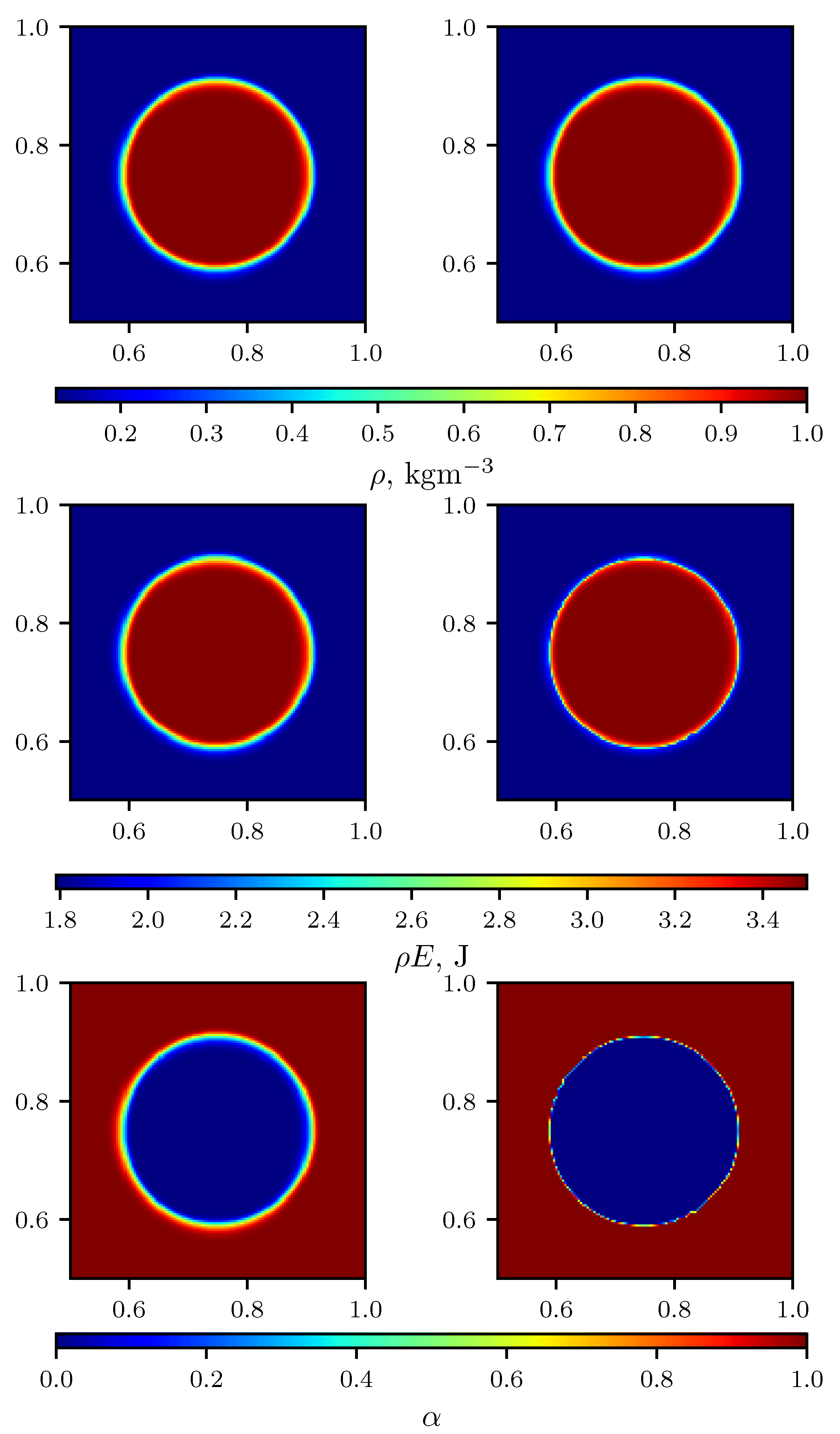
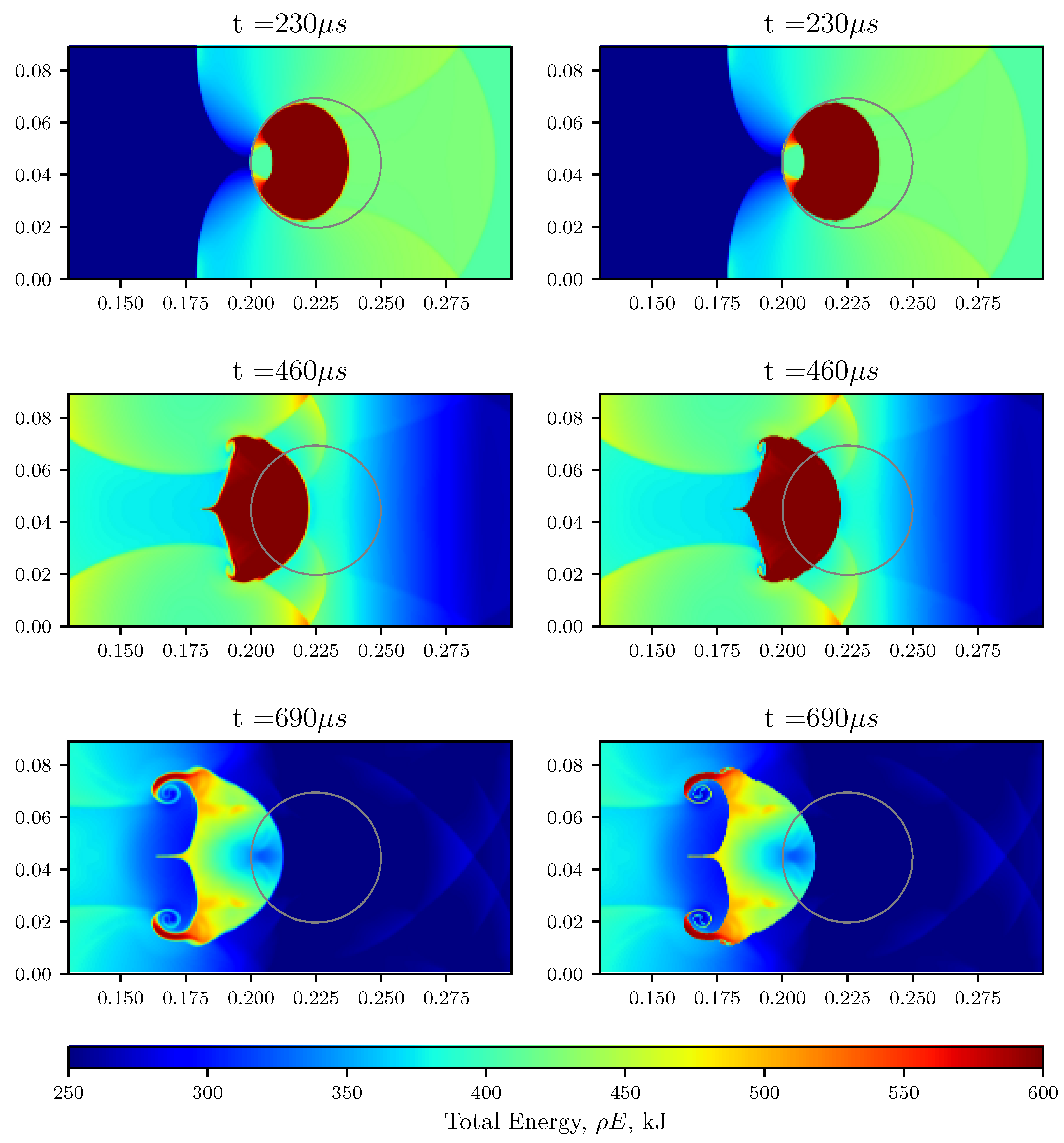
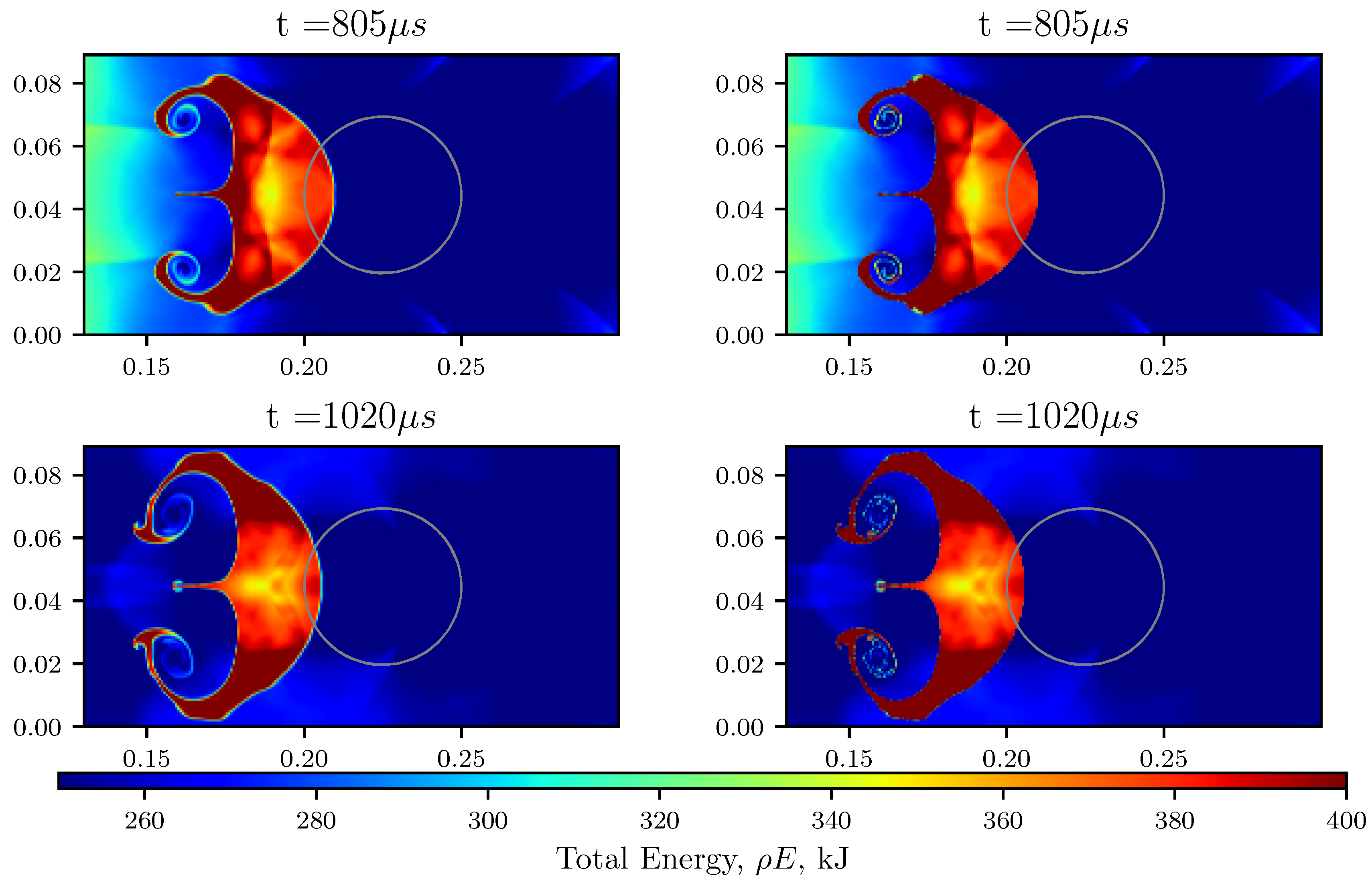
4.2.3. Shock-Bubble Interaction

Next, we consider the well-known shock-bubble interaction (see Figure 10), where a planar Mach 1.22 shock wave moving from right to left collides with an R22 bubble in air. This test-case effectively deals with the two species, R22 and air, modelled as ideal gases ($p_{\infty }=0$). Different variations of this test-case exist in the literature [20,27,44].

Here, we implement the test-case as described by Shyue et al. [27]. An R22 gas bubble with a radius of $R_0=25$ mm is centred at ${\mathit{x}}_c=\left(225,44.5\right)$ mm in a shock-tube of size $\left(x,y\right)\in [0,445]\times [0,89]$ mm${}^2$. The planar wave is located behind at $x=275$ mm, defining the pre- and post-shock regions, respectively,

$$\left(\rho ,\mathit{u},p,\gamma ,p_{\infty }\right)=\left\{\begin{array}{cc}\left(1.686{\mathrm{kgm}}^{-3},\left(-113.5,0\right){\mathrm{ms}}^{-1},1.59\times {10}^5\mathrm{Pa},1.4,0.0\right),\hfill & \mathrm{if}x\le 275mm,\hfill \\ \left(3.863{\mathrm{kgm}}^{-3},\left(0,0\right),1.01325\times {10}^5\mathrm{Pa},1.249,0.0\right),\hfill & \mathrm{if}|\mathit{x}-{\mathit{x}}_c|\le R_0,\hfill \\ \left(1.225{\mathrm{kgm}}^{-3},\left(0,0\right),1.01325\times {10}^5\mathrm{Pa},1.4,0.0\right),\hfill & \mathrm{if}x>275mm\cap |\mathit{x}-{\mathit{x}}_c| > R_0\hfill \end{array}\right.$$

The simulation is run on a 3560 × 356 node mesh at a CFL of 0.9 for a total time of 1020 µs.

Figure 11 and Figure 12 illustrate the evolution of total energy as a function of time and again HLLC is compared with CICSAM for the VoF equation. For the same adiabatic coefficient, the speed of sound inside the R22 gas bubble is slower compared to the air around. Hence, the wave generated inside the bubble is a rarefaction wave while the incoming wave is a shock wave. The interaction of these two waves produces two outgoing transmitted waves that get reflected at the boundary and free surfaces. These subsequent waves result in the denser fluid (R22) being decelerated by the lighter fluid (air). These lead to the appearance of Rayleigh–Taylor instabilities as illustrated at $t=690-1020$μs. For the purpose of comparison with experimental data, the Schlieren-type images are shown in Figure 13.

Qualitatively, the plots show flow features that are consistent with numerical results illustrated in (Figure 5) in [27] with similar improvements as previously discussed with respect to the VoF and energy field seen when using CICSAM.

4.2.4. Spurious Currents in a Static Bubble

A classic test-case [1,34,51,53] to validate surface tension schemes is that of a static bubble. It is employed here to validate the accuracy of both HLLC and CICSAM VoF methods in conjunction with height function and convolution curvature calculation. An ideal gas bubble with radius $R_0=0.4$ is initialised in a slightly compressible liquid at the centre of a unit domain. The material properties are set as per Fuster et al. [12]:

$$\left({\rho }_1,{\gamma }_1,p_{{\infty }_1}\right) = \left(1.0,1.4,0.0\right)\mathrm{and}\left({\rho }_2,{\gamma }_2,p_{{\infty }_2}\right) = \left(1.0,7.14,300\right),$$

with $\sigma =1$ and where the grid is such that $\frac{R_0}{\Delta x}=12.4$ (equispaced structured). A uniform pressure field is initialised. The simulation is run for 15 s (≈179,229 steps at $\Delta t\approx 8$e${}^{-5}$) to allow the system to reach steady state. The infinity norm of the maximum pressure jump, $\parallel {\epsilon }_{\Delta p}{\parallel }_{\infty }$, is computed using

$$\parallel {\epsilon }_{\Delta p}{\parallel }_{\infty }=\frac{|\Delta p_{nu}-\Delta p_{an}|}{\Delta p_{an}},$$

where $\Delta p$ is the difference between the maximum and minimum pressure in the domain, with $p_{nu}$ and $p_{an}$ the numerical and analytical pressure, respectively. Further, the velocity is non-dimensionalised with respect to the characteristic inviscid velocity $U_{\sigma }$, which is computed as per Popinet et al. [50]:

$$U_{\sigma }=\sqrt{{\displaystyle \frac{\sigma }{2\rho R_0}}}.$$

The quantitative results are summarized in

Table 1. Magnitude of max. dimensionless velocity and pressure jump error at $t=15$ s.

Capturing Scheme	$\mathit{\kappa }$	${|\mathit{u}|}_{\mathit{max}}/{\mathit{U}}_{\mathit{\sigma }}$	${\parallel \mathit{\epsilon }(\mathbf{\Delta }\mathit{p})\parallel }_{\mathit{\infty }}$
HLLC	Height	2.83 × 10${}^{-2}$	4.15 × 10${}^{-2}$
HLLC-CICSAM	Height	6.54 × 10${}^{-9}$	3.20 × 10${}^{-3}$
HLLC	Convolution	5.98 × 10${}^{-3}$	8.74 × 10${}^{-3}$
HLLC-CICSAM	Convolution	2.40 × 10${}^{-1}$	1.27 × 10${}^{-1}$

showing the clear superiority of CICSAM with height functions if used on a Cartesian mesh. Figure 14 illustrates the evolution of the velocity currents over time. The maximum velocity recorded with CICSAM and height functions is of the order of 10${}^{-8}$ while that with HLLC is divergent. This shows that the proposed scheme is well-balanced as well as the importance of accurate curvature calculation. The errors when using convolution to compute a pressure jump are significantly higher due to a larger error in curvature similar to [54].

4.2.5. Oscillating Bubble

A more challenging test-case [1,29,53,55,56] to validate the implementation of surface tension effects in the solver is to simulate the periodic deformation of a liquid droplet in air in the absence of gravity. The equation for the initially deformed droplet, as per Torres et al. [55], is given in polar coordinates as

$$r\left(\theta \right)=R_0+{ϵ}_{r}cos\left(n\theta \right),$$

where n is the integer mode of oscillation and $R_0$ is the initial radius. Here for $n=2$, the above equation is written in Cartesian coordinates as

$$\left(x^2+y^2\right)-{\left({ϵ}_r\left[\frac{x^2-y^2}{x^2+y^2}+R_0\right]\right)}^2=0,$$

with ${ϵ}_r=0.01$ and $R_0=0.8$.

The thermodynamic properties for the EOS are given as per Garrick et al. [1]:

$$\begin{array}{c}\hfill \left({\gamma }_1,p_{{\infty }_1}\right)=\left(1.4,0.0\right)\mathrm{and}\left({\gamma }_2,p_{{\infty }_2}\right)=\left(4.4,6000\right),\end{array}$$

where the densities of the gas and liquid are ${\rho }_1=0.01$ and ${\rho }_2=1$ with $\sigma =1$. The theoretical small-amplitude inviscid oscillation frequency is then

$${\omega }_n^2=\frac{\left(n^3-n\right)\sigma }{\left({\rho }_1+{\rho }_2\right)R_0^3}.$$

The domain is a square of size $[-2,2]$ m and the velocity field is initialised to zero everywhere. The simulation is run for a total time of two periods, using a CFL of 0.4. Figure 15 illustrates the evolution of the overall kinetic energy where the damping is due to the presence of numerical dissipation at low mesh resolution as seen in the work by Garrick et al. [1]. Here, the maximum % error, as compared to the analytical period on the coarsest mesh, is 1.1%, while on the finest, it is 0.15%. The results are comparable to those obtained by others [29,55,56]. As shown in Figure 16, second-order convergence is recovered while refining from a ${200}^2$ to ${400}^2$ mesh.

4.2.6. Rayleigh–Plesset Collapse Problem

A popular test-case [12,40,57] to evaluate the effect of non-linear terms in multi-phase compressible flow is the so called Rayleigh–Plesset bubble expansion–contraction problem [58]. Here, we consider a cylindrical bubble (2-D) in an incompressible liquid. A gas bubble of radius $R_0$ at initial pressure $p_{b,0}$ expands and contracts in an incompressible liquid due to a sudden change in the surrounding pressure. The evolution of the radius is governed by the Rayleigh–Plesset model [59]. The initial pressure field is

$$p(r,0)=p_{b,0}-\frac{\sigma }{R_0}-\frac{ln\left(\frac{r}{R_0}\right)}{ln\left(\frac{S}{R_0}\right)}\left[p_{b,0}-\frac{\sigma }{R_0}-p_{S,0}\right].$$

(44)

where R, $\dot{R}$, $\ddot{R}$ are the bubble radius, interface velocity and acceleration of the bubble, respectively. Further, $p_{S,0}$ is the initial pressure at a finite distance S.

For the purpose of simulating the problem, a bubble of radius $R_0=2$ µm is first initialised at the centre of a square domain of size $[-5,5]$ µm and a Cartesian mesh is employed. The driving pressure function at the outer boundary is expressed as

$$p_S\left(t\right)=200(1+0.1sin\left(10{\omega }_{c}t\right)),$$

(45)

where ${\omega }_c=10208967.75$ s${}^{-1}$ as per [59,60]. The material properties are as per Fuster et al. [12]:

$$\begin{array}{cc}\hfill & \left({\rho }_1,p_b,{\gamma }_1,p_{{\infty }_1}\right)=\left({10}^{-3},100,1.4,0.0\right),\hfill \\ \hfill & \left({\rho }_2,p_2,{\gamma }_2,p_{{\infty }_2}\right)=\left(1.0,200,7.14,3\times {10}^4\right),\hfill \end{array}$$

with $\sigma =0.1$. At each iteration, a Dirichlet pressure boundary condition (pulse) is set at the outer boundary as per (46). The simulation is run at a CFL number of 0.5 for 0.5 s.

Figure 17 illustrates a time lag on the numerical solution with an overshoot on rebound, which is invariant with respect to mesh refinement. This “incorrect” solution is due to the use of a finite Cartesian domain where such effects were first seen in [40]. To demonstrate this and also to show the applicability of the scheme developed in this paper to non-orthogonal grids, the calculation is repeated using a curvilinear mesh of radius 5 µm where elements are grown in size outside of the bubble. Since height functions are limited to structured grids, the convolution method is used for the curvature calculation.

Figure 18 illustrates that the numerical solution now asymptotes to the analytical, correcting the time lag and overshoot in Figure 17. In

Table 2. Rayleigh–Plesset problem (curvilinear mesh (circular domain)): error in minimum radius ($R_{min}$), time period (T) and radius of rebound ($R_r$).

$\frac{{\mathit{R}}_0}{\mathbf{\Delta }\mathit{x}}$	${\mathit{\epsilon }}_{\mathit{r}}\left({\mathit{R}}_{\mathit{min}}\right)\%$	${\mathit{\epsilon }}_{\mathit{r}}\left(\mathit{T}\right)\%$	${\mathit{\epsilon }}_{\mathit{r}}\left({\mathit{R}}_{\mathit{r}}\right)\%$
20	4.90	2.19	0.001522
40	2.43	0.91	0.001405
80	1.23	0.49	0.001375

, the relative error on the minimum radius of collapse, the time period and the amplitude of rebound are recorded. Here, a maximum error of 4.9% is noted on the minimum radius on the coarsest mesh and 1.2% on the finest mesh. Satisfactory convergence with the analytical solution is obtained on the finest mesh ($\frac{R}{\Delta x}=80$). Figure 19 illustrates the evolution of the bubble at the start, mid-way and end time of the simulation. As shown, the CICSAM algorithm allows for sharp capturing of the interface retaining the geometric integrity of the bubble. This test-case demonstrates that the scheme can accurately predict the non-linear collapse of a poly-tropic gas bubble.

5. Conclusions

In this article, we have presented an all-Mach HLLC-based scheme capable of accurately modelling a homogeneous compressible two-phase flow in the presence of surface tension. The solver for the first time combines HLLC (with primitive variable reconstruction) and the conservative VoF CICSAM method for the sharp propagation of the interface. Here, the reconstruction of primitive variables allowed for the consistent integration of the VoF and energy flux where the ECC was satisfied. The addition of CICSAM to HLLC allowed for the accurate calculation of interface curvature and therefore accurate capture of surface tension effects.

References

1. Garrick, D.P.; Owkes, M.; Regele, J.D. A finite-volume HLLC-based scheme for compressible interfacial flows with surface tension. J. Comput. Phys. 2017, 339, 46–67. [Google Scholar] [CrossRef] [Green Version]
2. Sussman, M. A second order coupled level set and volume-of-fluid method for computing growth and collapse of vapor bubbles. J. Comput. Phys. 2003, 187, 110–136. [Google Scholar] [CrossRef]
3. Cummins, S.; Francois, M.; Kothe, D. Estim. Curvature Vol. Fractions. Comput. Struct. 2005, 83, 425–434. [Google Scholar] [CrossRef]
4. Brackbill, J.; Kothe, D.; Zemach, C. A Continuum Method for Modeling Surface-Tension. J. Comput. Phys. 1992, 100, 335–354. [Google Scholar] [CrossRef]
5. Xu, Z.; Wu, F.; Yang, X.; Li, Y. Measurement of Gas-Oil Two-Phase Flow Patterns by Using CNN Algorithm Based on Dual ECT Sensors with Venturi Tube. Sensors 2020, 20, 1200. [Google Scholar] [CrossRef] [Green Version]
6. Roshani, M.; Phan, G.; Roshani, G.H.; Hanus, R.; Nazemi, B.; Corniani, E.; Nazemi, E. Combination of X-ray tube and GMDH neural network as a nondestructive and potential technique for measuring characteristics of gas-oil-water three phase flows. Measurement 2021, 168. [Google Scholar] [CrossRef]
7. Fang, L.; Zeng, Q.; Wang, F.; Faraj, Y.; Zhao, Y.; Lang, Y.; Wei, Z. Identification of two-phase flow regime using ultrasonic phased array. Flow Meas. Instrum. 2020, 72. [Google Scholar] [CrossRef]
8. Roshani, M.; Phan, G.T.T.; Ali, P.J.M.; Roshani, G.H.; Hanus, R.; Duong, T.; Corniani, E.; Nazemi, E.; Kalmoun, E.M. Evaluation of flow pattern recognition and void fraction measurement in two phase flow independent of oil pipeline’s scale layer thickness. Alex. Eng. J. 2021, 60, 1955–1966. [Google Scholar] [CrossRef]
9. Signor, L.; Dragon, A.; Roy, G.; De Resseguier, T.; Llorca, F. Dynamic fragmentation of melted metals upon intense shock wave loading. Some modelling issues applied to a tin target. Arch. Mech. 2008, 60, 323–343. [Google Scholar]
10. Milne, A.; Longbottom, A.; Frost, D.L.; Loiseau, J.; Goroshin, S.; Petel, O. Explosive fragmentation of liquids in spherical geometry. Shock Waves 2017, 27, 383–393. [Google Scholar] [CrossRef] [Green Version]
11. Milne, A.M.; Parrish, C.; Worland, I. Dynamic fragmentation of blast mitigants. Shock Waves 2010, 20, 41–51. [Google Scholar] [CrossRef]
12. Fuster, D.; Popinet, S. An all-Mach method for the simulation of bubble dynamics problems in the presence of surface tension. J. Comput. Phys. 2018, 374, 752–768. [Google Scholar] [CrossRef] [Green Version]
13. Durand, O.; Jaouen, S.; Soulard, L.; Heuze, O.; Colombet, L. Comparative simulations of microjetting using atomistic and continuous approaches in the presence of viscosity and surface tension. J. Appl. Phys. 2017, 122. [Google Scholar] [CrossRef]
14. Baer, M.R.; Nunziato, J.W. A two-phase mixture theory for the Deflagaration—to—Detonation Transition (DDT) in reactive Granular Materials. Int. J. Multiph. Flow 1986, 12, 861–889. [Google Scholar] [CrossRef]
15. Saurel, R.; Abgrall, R. A Multiphase Godunov Method for Compressible Multifluid and Multiphase Flows. J. Comput. Phys. 1999, 150, 425–467. [Google Scholar] [CrossRef]
16. Tian, B.; Toro, E.F.; Castro, C.E. A path-conservative method for a five-equation model of two-phase flow with an HLLC-type Riemann solver. Comput. Fluids 2011, 46, 122–132. [Google Scholar] [CrossRef]
17. Pelanti, M.; Shyue, K.M. A mixture-energy-consistent numerical approximation of a two-phase flow model for fluids with interfaces and cavitation. Am. Inst. Math. Sci. 2014, 839–846. [Google Scholar]
18. Furfaro, D.; Saurel, R. A simple HLLC-type Riemann solver for compressible non-equilibrium two-phase flows. Comput. Fluids 2015, 111, 159–178. [Google Scholar] [CrossRef]
19. Kapila, A.; Menikoff, R.; Bdzil, J.; Son, S.; Stewart, D. Two-phase modeling of deflagration-to-detonation transition in granular materials: Reduced equations. Phys. Fluids 2001, 13, 3002–3024. [Google Scholar] [CrossRef]
20. Daude, F.; Galon, P.; Gao, Z.; Blaud, E. Numerical experiments using a HLLC-type scheme with ALE formulation for compressible two-phase flows five-equation models with phase transition. Comput. Fluids 2014, 94, 112–138. [Google Scholar] [CrossRef]
21. He, Z.; Tian, B.; Zhang, Y.; Gao, F. Characteristic-based and interface-sharpening algorithm for high-order simulations of immiscible compressible multi-material flows. J. Comput. Phys. 2017, 333, 247–268. [Google Scholar] [CrossRef]
22. Jibben, Z.; Velechovsky, J.; Masser, T.; Francois, M.M. Modeling surface tension in compressible flow on an adaptively refined mesh. Comput. Math. Appl. 2019, 78, 504–516. [Google Scholar] [CrossRef]
23. Ilangakoon, N.A.; Malan, A.G.; Jones, B.W.S. A higher-order accurate surface tension modelling volume-of-fluid scheme for 2D curvilinear meshes. J. Comput. Phys. 2020, 420. [Google Scholar] [CrossRef]
24. Heyns, J.A.; Malan, A.G.; Harms, T.M.; Oxtoby, O.F. A weakly compressible free-surface flow solver for liquid-gas systems using the volume-of-fluid approach. J. Comput. Phys. 2013, 240, 145–157. [Google Scholar] [CrossRef]
25. Oxtoby, O.F.; Malan, A.G.; Heyns, J.A. A computationally efficient 3D finite-volume scheme for violent liquid-gas sloshing. Int. J. Numer. Methods Fluids 2015, 79, 306–321. [Google Scholar] [CrossRef]
26. Malan, L.C.; Malan, A.G.; Zaleski, S.; Rousseau, P.G. A geometric VOF method for interface resolved phase change and conservative thermal energy advection. J. Comput. Phys. 2021, 426. [Google Scholar] [CrossRef]
27. Shyue, K. A wave-propagation based volume tracking method for compressible multicomponent flow in two space dimensions. J. Comput. Phys. 2006, 215, 219–244. [Google Scholar] [CrossRef]
28. Corot, T.; Hoch, P.; Labourasse, E. Surface tension for compressible fluids in ALE framework. J. Comput. Phys. 2020, 407. [Google Scholar] [CrossRef]
29. Perigaud, G.; Saurel, R. A compressible flow model with capillary effects. J. Comput. Phys. 2005, 209, 139–178. [Google Scholar] [CrossRef]
30. Toro, E.F.; Spruce, M.; Speares, W. Restoration of the contact surface in the HLL-Riemann solver. Shock Waves 1994, 4, 25–34. [Google Scholar] [CrossRef]
31. Roe, P. Approximate Riemann solvers, parameter vectors, and difference schemes. J. Comput. Phys. 1981, 43, 357–372. [Google Scholar] [CrossRef]
32. Xiao, F. Unified formulation for compressible and incompressible flows by using multi-integrated moments I: One-dimensional inviscid compressible flow. J. Comput. Phys. 2004, 195, 629–654. [Google Scholar] [CrossRef]
33. Chiapolino, A.; Saurel, R.; Nkonga, B. Sharpening diffuse interfaces with compressible fluids on unstructured meshes. J. Comput. Phys. 2017, 340, 389–417. [Google Scholar] [CrossRef] [Green Version]
34. Ubbink, O.; Issa, R. A method for capturing sharp fluid interfaces on arbitrary meshes. J. Comput. Phys. 1999, 153, 26–50. [Google Scholar] [CrossRef] [Green Version]
35. Mirjalili, B.S.; Jain, S.S.; Dodd, M.S. Interface-capturing methods for two-phase flows: An overview and recent developments. In Annual Research Briefs; Center for Turbulence Research: Stanford, CA, USA, 2017; pp. 117–135. [Google Scholar] [CrossRef]
36. Weymouth, G.D.; Yue, D.K.P. Conservative Volume-of-Fluid method for free-surface simulations on Cartesian-grids. J. Comput. Phys. 2010, 229, 2853–2865. [Google Scholar] [CrossRef]
37. Zhang, D.; Jiang, C.; Liang, D.; Chen, Z.; Yang, Y.; Shi, Y. A refined volume-of-fluid algorithm for capturing sharp fluid interfaces on arbitrary meshes. J. Comput. Phys. 2014, 274, 709–736. [Google Scholar] [CrossRef] [Green Version]
38. Ivey, C.B.; Moin, P. Conservative and bounded volume-of-fluid advection on unstructured grids. J. Comput. Phys. 2017, 350, 387–419. [Google Scholar] [CrossRef]
39. Malan, A.G.; Oxtoby, O.F. An accelerated, fully-coupled, parallel 3D hybrid finite-volume fluid-structure interaction scheme. Comput. Methods Appl. Mech. Eng. 2013, 253, 426–438. [Google Scholar] [CrossRef]
40. Malan, L.C.; Ling, Y.; Scardovelli, R.; Llor, A.; Zaleski, S. Detailed numerical simulations of pore competition in idealized micro-spall using the VOF method. Comput. Fluids 2019, 189, 60–72. [Google Scholar] [CrossRef]
41. Van Leer, B. Towards the ultimate conservative difference scheme. V. A second-order sequel to Godunov’s method. J. Comput. Phys. 1979, 32, 101–136. [Google Scholar] [CrossRef]
42. Pattinson, J.; Malan, A.G.; Meyer, J.P. A cut-cell non-conforming Cartesian mesh method for compressible and incompressible flow. Int. J. Numer. Methods Eng. 2008, 72, 1332–1354. [Google Scholar] [CrossRef]
43. Oxtoby, O.F.; Malan, A.G. A matrix-free, implicit, incompressible fractional-step algorithm for fluid-structure interaction applications. J. Comput. Phys. 2012, 231, 5389–5405. [Google Scholar] [CrossRef]
44. Johnsen, E.; Colonius, T. Implementation of WENO schemes in compressible multicomponent flow problems. J. Comput. Phys. 2006, 219, 715–732. [Google Scholar] [CrossRef]
45. Shyue, K.M. An Efficient Shock-Capturing Algorithm for Compressible Multicomponent Problems. J. Comput. Phys. 1998, 142, 208–242. [Google Scholar] [CrossRef] [Green Version]
46. Le Metayer, O.; Saurel, R. The Noble-Abel Stiffened-Gas equation of state. Phys. Fluids 2016, 28. [Google Scholar] [CrossRef] [Green Version]
47. Van Albada, G.D.; van Leer, B.; Roberts, W.W. A Comparative Study of Computational Methods in Cosmic Gas Dynamics. In Upwind and High-Resolution Schemes; Springer: Berlin/Heidelberg, Germany, 1997; pp. 95–103. [Google Scholar] [CrossRef] [Green Version]
48. Batten, P.; Clarke, N.; Lambert, C.; Causon, D.M. On the choice of wavespeeds for the HLLC riemann solver. SIAM J. Sci. Comput. 1997, 18, 1553–1570. [Google Scholar] [CrossRef]
49. Einfeldt, B.; Munz, C.; Roe, P.; Sjogreen, B. On Godunov-Type Methods near Low-Densities. J. Comput. Phys. 1991, 92, 273–295. [Google Scholar] [CrossRef]
50. Popinet, S. An accurate adaptive solver for surface-tension-driven interfacial flows. J. Comput. Phys. 2009, 228, 5838–5866. [Google Scholar] [CrossRef] [Green Version]
51. Popinet, S. Numerical Models of Surface Tension. Annu. Rev. Fluid Mech. 2018, 50, 49–75. [Google Scholar] [CrossRef] [Green Version]
52. Jones, B.W.S.; Malan, A.G.; Ilangakoon, N.A. The initialisation of volume fractions for unstructured grids using implicit surface definitions. Comput. Fluids 2019, 179, 194–205. [Google Scholar] [CrossRef]
53. Popinet, S.; Zaleski, S. A front-tracking algorithm for accurate representation of surface tension. Int. J. Numer. Methods Fluids 1999, 30, 775–793. [Google Scholar] [CrossRef]
54. Afkhami, S.; Bussmann, M. Height functions for applying contact angles to 2D VOF simulations. Int. J. Numer. Methods Fluids 2008, 57, 453–472. [Google Scholar] [CrossRef]
55. Torres, D.J.; Brackbill, J.U. The Point-Set Method: Front-Tracking without Connectivity. J. Comput. Phys. 2000, 165, 620–644. [Google Scholar] [CrossRef] [Green Version]
56. Fuster, D.; Agbaglah, G.; Josserand, C.; Popinet, S.; Zaleski, S. Numerical simulation of droplets, bubbles and waves: State of the art. Fluid Dyn. Res. 2009, 41. [Google Scholar] [CrossRef]
57. Popinet, S.; Zaleski, S. Bubble collapse near a solid boundary: A numerical study of the influence of viscosity. J. Fluid Mech. 2002, 464, 137–163. [Google Scholar] [CrossRef] [Green Version]
58. Plesset, M.; Prosperetti, A. Bubble Dynamics and Cavitation. Annu. Rev. Fluid Mech. 1977, 9, 145–185. [Google Scholar] [CrossRef]
59. Jain, S.S.; Mani, A.; Moin, P. A conservative diffuse-interface method for compressible two-phase flows. J. Comput. Phys. 2020, 418. [Google Scholar] [CrossRef]
60. Minnaert, M. XVI. On musical air-bubbles and the sounds of running water. Lond. Edinb. Dublin Philos. Mag. J. Sci. 1933, 16, 235–248. [Google Scholar] [CrossRef]
Figure 1. 2-D computational median dual-cell around node l.
Applsci 11 03413 g001
Figure 2. Elementary wave configuration to the Riemann Problem.
Applsci 11 03413 g002
Figure 3. Gas–liquid Riemann problem: assessment of Hartens–Lax–van Leer Contact (HLLC) and HLLC-compressive interface capturing scheme for arbitrary meshes (CICSAM)—100 nodes: The first row depicts the total internal energy (left) and velocity (right). The second row shows the pressure (left) and volume fraction field (right).
Applsci 11 03413 g003
Figure 4. Gas–liquid: assessment of HLLC vs. CICSAM—400, 800 and 1600 nodes.
Applsci 11 03413 g004
Figure 5. Advecting bubble: HLLC (left) and HLLC-CICSAM (right) on a 512 2 mesh.
Applsci 11 03413 g005
Figure 6. Advecting bubble: L 1 norm error.
Applsci 11 03413 g006
Figure 7. Underwater explosion: Schlieren-type images of density field for HLLC-CICSAM.
Applsci 11 03413 g007
Figure 8. Underwater explosion: HLLC (left) vs. HLLC-CICSAM (right). The first, second and third rows depict the evolution of the total energy field, respectively, at 0.4 , 1.2 and 2.5 ms.
Applsci 11 03413 g008
Figure 9. Underwater explosion: pressure plot across x = 0.
Applsci 11 03413 g009
Figure 10. Shock-bubble interaction: initial setup.
Applsci 11 03413 g010
Figure 11. Shock-bubble interaction: HLLC (left) vs. HLLC-CICSAM (right).
Applsci 11 03413 g011
Figure 12. Shock-bubble interaction: HLLC (left) vs. HLLC-CICSAM (right).
Applsci 11 03413 g012
Figure 13. Shock-bubble interaction: Schlieren-type images of the density field for HLLC-CICSAM.
Applsci 11 03413 g013
Figure 14. Evolution of spurious velocities over time.
Applsci 11 03413 g014
Figure 15. Oscillating bubble: computed kinetic energy evolution.
Applsci 11 03413 g015
Figure 16. Oscillating bubble: relative error on time period of oscillation.
Applsci 11 03413 g016
Figure 17. Rayleigh–Plesset problem (Cartesian mesh): predicted bubble radius evolution.
Applsci 11 03413 g017
Figure 18. Rayleigh–Plesset problem (curvilinear mesh (circular domain)): predicted bubble radius evolution.
Applsci 11 03413 g018
Figure 19. Rayleigh–Plesset problem: evolution of volume fraction field.
Applsci 11 03413 g019