Towards Improving Transparency of Count Data Regression Models for Health Impacts of Air Pollution

Abstract

In studies on the health impacts of air pollution, regression analysis continues to advance far beyond classical linear regression, which many scientists may have become familiar with in an introductory statistics course. With each new level of complexity, regression analysis may become less transparent, even to the analyst working with the data. This may be especially true in count data regression models, where the response variable (typically given the symbol y) is count data (i.e., takes on values of 0, 1, 2, …). In such models, the normal distribution (the familiar bell-shaped curve) for the residuals (i.e., the differences between the observed values and the values predicted by the regression model) no longer applies. Unless care is taken to correctly specify just how those residuals are distributed, the tendency to accept untrue hypotheses may be greatly increased. The aim of this paper is to present a simple histogram of predicted and observed count values (POCH), which, while rarely found in the environmental literature but presented in authoritative statistical texts, can dramatically reduce the risk of accepting untrue hypotheses. POCH can also increase the transparency of count data regression models to analysts themselves and to the scientific community in general.

1. Introduction

In count data regression analysis, the response variable takes on count values (i.e., 0, 1, 2, …). The consequences of this property of the response variable can be understood by comparison with classical linear regression analysis.

In classical linear regression analysis, for a set of $n$ datapoints, the predicted value of the response variable ${\widehat{y}}_i$ may be given by

$${\widehat{y}}_i={\widehat{\beta }}_0+{\widehat{\beta }}_1{x}_1{}_i+{\widehat{\beta }}_2{x}_2{}_i+\dots +{\widehat{\beta }}_m{x}_m{}_i for i=1, 2, \dots , n$$

(1)

where $x_1,\dots ,x_m$ are the covariates, ${\widehat{\beta }}_0,\dots ,{\widehat{\beta }}_m$ are the parameters, and ${\widehat{y}}_i$ is the predicted value of the response variable. ${\widehat{y}}_i$ is also the estimate of the expected value of the response variable given the covariate values. Hence, (1) is referred to as the conditional mean model (CMM).

The CMM residuals, i.e., the differences between ${\widehat{y}}_i$ and observed values $y_i$, are distributed about the conditional mean according to the normal probability density function (pdf):

$$f\left(re{s}_i\right)=\frac{1}{\sigma \sqrt{2\pi }}\exp \left(-\frac{1}{2}{\left(\frac{re{s}_i}{\sigma }\right)}^2\right)$$

(2)

where $re{s}_i=y_i-{\widehat{y}}_i$, the residual for the $i-{\mathrm{th}}^{}$ observed value, and $\sigma$ is the standard deviation of the residuals. The closer $re{s}_i$ is to 0, the higher the value of $f\left(re{s}_i\right)$. If the residuals are also identically distributed (i.e., come from the same, vast, imaginary pool of residuals) and independently distributed (i.e., one residual is not useful in predicting the value of another), then the pdfs may be multiplied together to form the normal-based likelihood function:

$$\begin{array}{c}{ℒ}_{normal}={\displaystyle {\displaystyle \prod }_{i=1}^n}\frac{1}{\sigma \sqrt{2\pi }}\exp \left(-\frac{1}{2}{\left(\frac{re{s}_i}{\sigma }\right)}^2\right)\hfill \\ ={\displaystyle {\displaystyle \prod }_{i=1}^n}\frac{1}{\sigma \sqrt{2\pi }}\exp \left(-\frac{1}{2}{\left(\frac{y_i-\left({\widehat{\beta }}_0+{\widehat{\beta }}_1{x}_1{}_i+{\widehat{\beta }}_2{x}_2{}_i+\dots +{\widehat{\beta }}_m{x}_m{}_i\right)}{\sigma }\right)}^2\right)\hfill \end{array}$$

(3)

The best estimates of CMM parameters may be found by adjusting them until they maximize this normal-based likelihood function.

Several properties of this likelihood function allow classical regression analysis to be transparent, both to the analyst working with the data and to the general audience reviewing the published results. Maximizing the likelihood function corresponds to minimizing the sum of the squares of the residuals, and thus a plot of the resulting conditional mean shows it passing more-or-less through the middle of the scattering of observed values. One senses that shifting or rotating that best-fit line would not improve the fit. Also, the relatively simple R², which varies from 0 to 1, and is a measure of the portion of the variation in the response variable accounted for by the conditional mean model, is visually represented in the plot.

In classical linear regression, the standard deviation appearing in the likelihood function can be estimated directly from the residuals to give a fairly reasonable representation of the spread of the data, even if the residuals are not exactly normally distributed. This, in turn, allows for p-values that tend to be relatively trustworthy. There is still a risk that a covariate that is not truly associated with the response variable will have a low p-value due to mere chance. This risk increases as the number of covariates under consideration for inclusion in the CMM increases. Overfitting of the CMM (i.e., the inclusion of covariates or other complexities that represent merely random effects rather than actual associations) may then occur. However, the dataset can be divided into two subsets—training data (to build the CMM) and testing data. The training data can be further subdivided for k-fold cross-validation, with reductions in R² or other simple measures to help detect the presence of inappropriate covariates. Finally, because such covariates may elude even k-fold cross-validation, the final CMM is applied to the testing data, and, again, reductions in R² or other simple measures will further aid in detecting false inference and overfitting.

Unfortunately, many of the above desirable features are not available in count data regression analysis. To begin with, the CMM immediately becomes more complex with the right side typically being exponentiated:

$${\widehat{y}}_i=e^{{\widehat{\beta }}_0+{\widehat{\beta }}_1{x}_1{}_i+{\widehat{\beta }}_2{x}_2{}_i+\dots +{\widehat{\beta }}_m{x}_m{}_i}$$

(4)

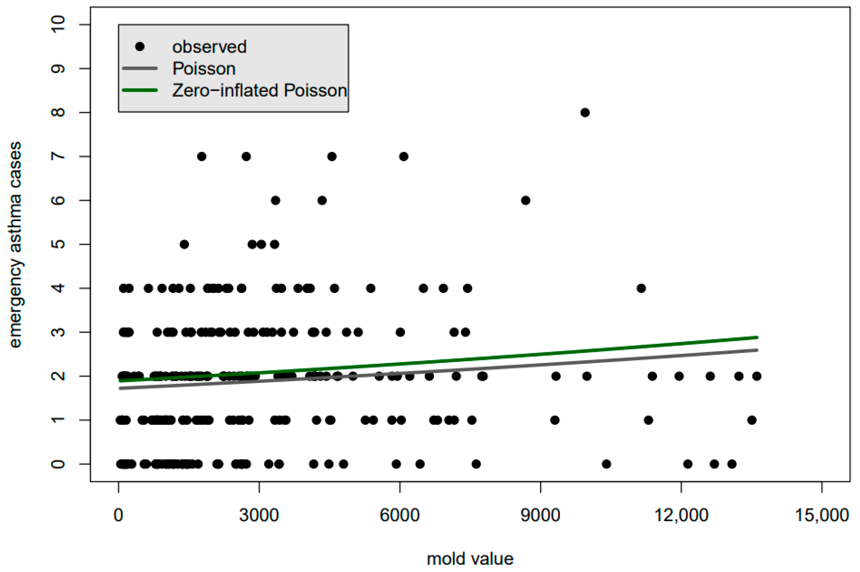
If one plots the conditional mean through the scattering of observed values, the correct placement of the line may now seem counter-intuitive because non-linearity in the CMM, along with other factors, mean that the distribution of the observed values will not likely be symmetric about the best fit line. Casual assessment of the goodness-of-fit by eye is difficult, as can be seen, for example, in Figure 1, which shows candidates of best-fit lines for childhood asthma data in Houston, Texas (Figure 1 will be discussed in more detail in the next section). Furthermore, the normal pdf will now need to be replaced by any one of dozens of probability mass functions (pmfs) to build the likelihood function. Incorrect pmf selection can lead to underestimation of the spread of the data, resulting in falsely low p-values [1], false inference, and overfitting. Worse still, there is no longer a simple, universally recognized R² or other intuitively appealing measures of goodness-of-fit that can be conveniently used in k-fold cross-validation or in application to test data to help warn against overfitting. There are only various forms of the more difficult to interpret pseudo-R², and other measures, depending on the representation of the residuals [2]. This may explain why authoritative “how-to” guides on data analysis in R may demonstrate k-fold cross-validation for various model types but not for count data regression [3,4]. In our literature review of the impact of air quality on respiratory health, we found k-fold cross-validation and application of testing data was used [5], but never for a count data response variable in a CMM.

Addressing all the ramifications of misspecification of the pmf in count data regression analysis is beyond the scope of this brief commentary. The impact of misspecification on p-values for covariate parameter estimates, and a simple strategy to reduce the tendency for the underestimation to occur, are illustrated in the following sections.

2. Illustration of False Inference and Overfitting Due to pmf Misspecification

The consequences of misspecifying the pmf in count data regression analysis can be seen in our own analysis of the relationship between air quality and childhood asthma in Houston, Texas, during the summers of 2003–2011. Concentrations of aeroallergens (mold and pollen) and anthropogenic contaminants (butane, nitrous oxide, ozone, sulfur dioxide, and particulates) were initially included in the model as covariates. The number of children arriving per day at particular hospital emergency departments for asthma was the response variable. We initially assumed the Poisson distribution for the pmf. With this pmf, a strong association between the response variable and the mold concentration was found, with p-value $<{10}^{-15}$.

However, the most appropriate CMM and pmf among those being considered may be identified as that which yields the lowest Akaike information criteria (AIC) value [6]

$$AIC=-2·ln(ℒ)+2·k$$

(5)

where $ℒ$ is the likelihood function value for the selected pmf, and $k$ is the number of parameters that may be adjusted to increase $ℒ$. The second term is thus a way of penalizing the inclusion of parameters, as including an additional adjustable parameter will always increase $ℒ$, even if the parameter is not truly representative of actual statistical relationships. Variations of the AIC may also be used. We use the original AIC here because it is commonly available in software packages. The chooseDist() function of the R gamlss package [7] runs through dozens of pmfs for building likelihood functions, adjusts parameters to maximize each, and then identifies the one with the lowest AIC. By using this process, dozens of pmfs were found, which yielded a lower AIC than did the Poisson distribution. An alternative pmf, the zero-inflated Poisson, which allows for a higher number of zeros than would be expected for the Poisson and thus, in turn, has a substantially broader spread than the Poisson would show for our dataset, was found to yield the lowest AIC among the dozens of available pmfs. The resulting p-value for the mold covariate was now 0.051, a p-value increase of many orders of magnitude compared to that provided by the Poisson pmf, leading the mold covariate to be accepted as statistically significant only under far less strict criteria.

Figure 1 shows a plot of the best-fit line through the data based on the Poisson pmf (gray) and the zero-inflated Poisson pmf (green). Due to the non-linearity of the CMM and other factors, one would be hard-pressed to say whether either of the lines fits the data well, let alone which fits the data better to justify the use of one CMM or pmf over the other. Indeed, as we will see in the following discussion of the generation and analysis of synthetic data, radically different pmfs may yield essentially identical CMMs, completely eliminating the usefulness of plots, such as in Figure 1, in determining which pmf is superior.

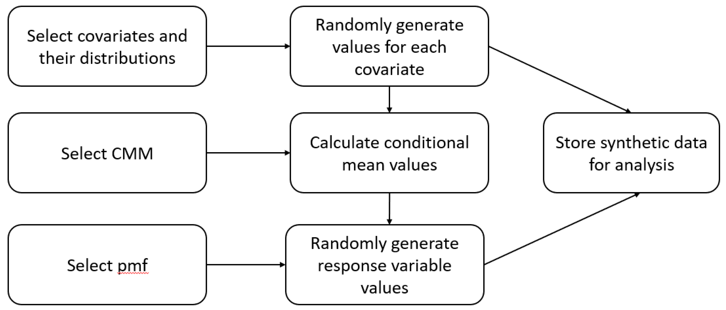
To show that the impact of pmf misspecification on p-values is not unique to peculiarities of the somewhat small air quality and childhood asthma dataset we ourselves are working with, we developed a synthetic dataset that readers are free to view, re-generate with parameters of their choice, and re-test through the link provided in the data availability statement below. Figure 2 shows how we generated the synthetic dataset and how the reader could use the code to generate their own. The three blocks forming the left column of the schematic are all the reader would need to select to build the synthetic dataset.

For our synthetic dataset, which we analyzed in

Table 1. Results for regression analysis using negative binomial (Neg. Bin.) pmf (${ℒ}_{optimal}$ columns) and Poisson pmf (${ℒ}_{Poisson}$ columns).

	$\widehat{\mathit{y}}={\mathit{e}}^{{\widehat{\mathit{\beta }}}_0+{\widehat{\mathit{\beta }}}_1{\mathit{x}}_1}$ as a Conditional Mean Model		$\widehat{\mathit{y}}={\mathit{e}}^{{\widehat{\mathit{\beta }}}_0+{\widehat{\mathit{\beta }}}_1{\mathit{x}}_1+{\widehat{\mathit{\beta }}}_2\mathit{x}}$ as a Conditional Mean Model		$\widehat{\mathit{y}}={\mathit{e}}^{{\widehat{\mathit{\beta }}}_0+{\widehat{\mathit{\beta }}}_1{\mathit{x}}_1+{\widehat{\mathit{\beta }}}_2\mathit{x}+{\widehat{\mathit{\beta }}}_3{\mathit{x}}_3}$ as a Conditional Mean Model
	${\mathit{ℒ}}_{\mathit{P}\mathit{o}\mathit{i}\mathit{s}\mathit{s}\mathit{o}\mathit{n}}$	${\mathit{ℒ}}_{\mathit{o}\mathit{p}\mathit{t}\mathit{i}\mathit{m}\mathit{a}\mathit{l}}$	${\mathit{ℒ}}_{\mathit{P}\mathit{o}\mathit{i}\mathit{s}\mathit{s}\mathit{o}\mathit{n}}$	${\mathit{ℒ}}_{\mathit{o}\mathit{p}\mathit{t}\mathit{i}\mathit{m}\mathit{a}\mathit{l}}$	${\mathit{ℒ}}_{\mathit{P}\mathit{o}\mathit{i}\mathit{s}\mathit{s}\mathit{o}\mathit{n}}$	${\mathit{ℒ}}_{\mathit{o}\mathit{p}\mathit{t}\mathit{i}\mathit{m}\mathit{a}\mathit{l}}$
pmf	Poisson	Neg. bin.	Poisson	Neg. bin.	Poisson	Neg. bin.
${\sigma }_i$	$\sqrt{{\widehat{y}}_i}$	$\sqrt{{\widehat{y}}_i+\alpha {\widehat{y}}_i{}^2}$	$\sqrt{{\widehat{y}}_i}$	$\sqrt{{\widehat{y}}_i+\alpha {\widehat{y}}_i{}^2}$	$\sqrt{{\widehat{y}}_i}$	$\sqrt{{\widehat{y}}_i+\alpha {\widehat{y}}_i{}^2}$
$\alpha$	NA	0.515	NA	0.512	NA	0.511
AIC	15,054.0	7905.6	14,973.3	7900.9	14,960.1	7901.3
${\widehat{\beta }}_0$ (p-value)	1.52 ($<2\times {10}^{-16})$	1.47 ($7.6\times {10}^{-9})$	0.85 ($7.2\times {10}^{-16}$)	0.84 (0.017)	1.15 $(<2\times {10}^{-16})$	1.17 (0.0072)
${\widehat{\beta }}_1$ (p-value)	0.15 ($<2\times {10}^{-16})$	0.15 ($1.2\times {10}^{-9}$)	0.15 ($<2\times {10}^{-16})$	0.15 ($1.1\times {10}^{-9})$	0.15 ($<2\times {10}^{-16})$	0.15 ($9.3\times {10}^{-10})$
${\widehat{\beta }}_2$ (p-value)	NA	NA	0.065 ($<2\times {10}^{-16})$	0.063 (0.0099)	0.064 $(<2\times {10}^{-16})$	0.063 (0.011)
${\widehat{\beta }}_3$ (p-value)	NA	NA	NA	NA	−0.029 $\left(0.00010\right)$	−0.033 (0.20)

below, the code provided through the link was applied in R version 4.0.0 [8] to generate 1000 values for each of three covariates, $x_1,$ $x_2$, and $x_3$, from the normal distribution with the mean $\mu =10$ and standard deviation $\sigma =1$. Parameter values were then assigned to create 1000 conditional mean values as follows, with $x_3$ excluded:

$${\widehat{y}}_i=e^{1+0.1x_1{}_i+0.1x_2{}_i} for i=1, 2,\dots , 1000$$

(6)

Observed $y_i$ values were distributed about these ${\widehat{y}}_i$ values according to the negative binomial pmf, which has a standard deviation of ${\sigma }_i=\sqrt{{\widehat{y}}_i+\alpha {\widehat{y}}_i^2}$. (This is in contrast with the Poisson distribution, which is less spread out, with ${\sigma }_i=\sqrt{{\widehat{y}}_i}$.) A value of 0.5 was chosen for $\alpha$, the dispersion parameter.

The results for each of the three CMMs are shown in Table 1 ${ℒ}_{optimal}$ columns. In each case, the optimal pmf is, not surprisingly, the same one used to generate the data. In some cases, adding covariates may cause a switch to a pmf with a less spread structure [1]. As expected, $x_3$, which was not used to generate the response variable, has a coefficient with a p-value well above 0.05, and slightly increases the AIC. It is to be excluded from the CMM.

For comparison, results for the Poisson pmf, often used in the literature, appear in the ${ℒ}_{Poisson}$ columns. The p-values are now falsely low, sometimes by several orders of magnitude. The false inference would now lead to including $x_3$. The lowering of the AIC value by including $x_3$ shows that the AIC is inadequate for preventing CMM overfitting.

Hilbe, an author of more than 10 books on statistical modeling, has cautioned that “Many analysts have been deceived into thinking that they have developed a well-fitted model” because the spread of the residuals was greater than represented in their count data regression model [1]. In our own dataset of childhood asthma and air quality in Houston, the distribution of the daily arrivals to the emergency department appears to be zero-inflated, i.e., there is an inexplicably high number of days with zero arrivals if the observed values are assumed to be Poisson distributed about the conditional mean. The zero-inflated Poisson pmf accounted for what is in effect an increase in the spread of the residuals, thereby giving a more realistic p-value (0.051), which is many orders of magnitude higher than that suggested by the Poisson pmf ($<{10}^{-15}$).

Utilizing the most appropriate pmf can dramatically reduce the risk of false inference and overfitting. However, it must be noted that the AIC and related criteria do not establish appropriateness in any absolute sense but only identify the best choice among a set of choices. It could be that none of the choices is ultimately appropriate. In recognition of this limitation of such criteria, and in recognition of limitations among various software packages to select the most appropriate pmf, and to provide an intuitively appealing visual check on the selected pmf and CMM, a predicted-and-observed count histogram (POCH) is discussed in the following section.

3. The Predicted-And-Observed Count Histogram

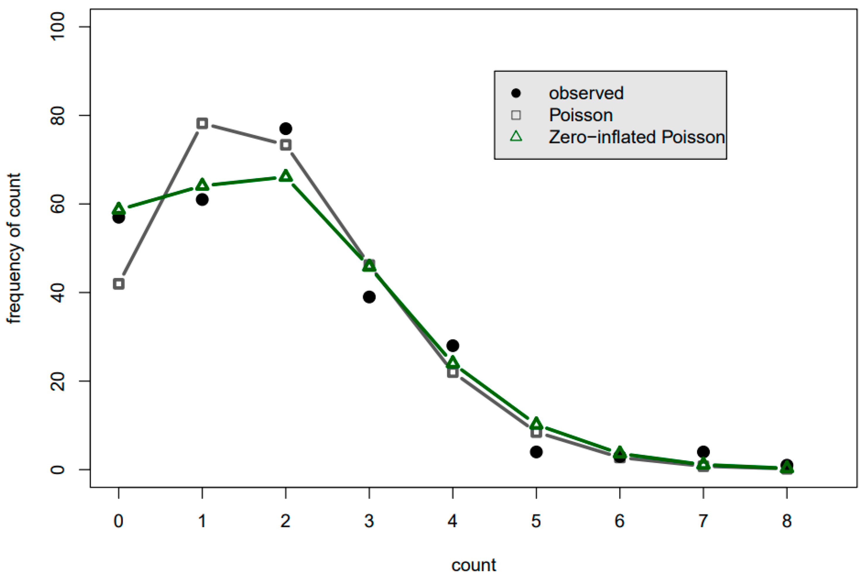
Figure 3 and Figure 4 are predicted-and-observed count histograms (POCH), similar to what is presented but not formally named in authoritative count data regression analysis texts [1,2]. Black dots and other markers are where the tops of the more traditional vertical histogram bars would be to represent the number of times that the response variable takes on the count value. The black dots represent the number of occurrences of the observed response variable values, while the green and gray markers represent the number of occurrences predicted by the models. In Figure 3, for example, the black dot at the count of 0 indicates that there were 0 childhood asthma emergency department arrivals on 57 of the summer days, while the gray square indicates that the Poisson pmf anticipates 0 arrivals to occur on only 40 of the summer days. Figure 3 shows that while the Poisson and zero-inflated Poisson had similar performance in predicting the number of days for which three or more arrivals occur, the zero-inflated Poisson pmf was a substantial improvement overall for the lower arrival numbers. In Figure 4, the model having two covariates and using the negative binomial pmf was clearly a better fit than was the three-covariate model with the Poisson pmf. Though not shown in either POCH, the analyst may generate predicted values from the pmf that best fits the observed histogram directly, i.e., without a CMM, note the resulting AIC value, and thus have a baseline AIC value from which to develop the CMM.

In both Figure 3 and Figure 4, the POCH shows Poisson pmfs (as opposed to the zero-inflated and negative binomial pmfs) have a more narrow distribution than does the actual data. It thus clearly warns that p-values with the Poisson pmf for these particular datasets will be falsely low. Such charts immediately provide transparency of the complicated count data regression analysis to the analyst working with the data and to the broader audience.

The POCH is easily generated for even the most complex count data regression analysis models, including ones that incorporate smoothing splines, autoregressive parameters, etc., as in generalized additive models and models in which the count data is binary, such as in case-crossover studies. The POCH merely requires a predicted response variable and a representation of the distribution of residuals, and so can be developed even for a quasi-likelihood method [9].

A POCH helps assess the correctness of the pmf not only in regards to spread, but also in regard to skewness, zero-inflation, hurdles, and other potentially important features. A POCH will not entirely address every violation of statistical assumptions. For example, one still needs to check for autocorrelation among residuals. However, where the POCH does not directly address them, it may provide a solid starting point. For example, testing for autocorrelation in count models requires standardizing the residuals before plotting the autocorrelation function [2,10]. The POCH can help identify the correct pmf for the standardization. Once the final model is selected, perhaps including autoregressive parameters, the POCH should be re-generated to re-confirm the appropriateness of the model.

In our literature review of the impact of air quality on health, we found no histogram such as a POCH, or any explicit evidence that the most appropriate pmf was used. This absence even among excellent articles [11,12,13,14,15,16,17,18] suggests a systemic issue extending beyond individual authors. We recommend that publishers require a POCH for articles involving count data regression models.

4. Conclusions

The complexity of count data regression models can lead to false inference and overfitting. A remedy is a predicted-and-observed count histogram POCH, which makes the analysis more transparent to analysts themselves and to the scientific community in general.