
Large-Scale Truss-Sizing Optimization with Enhanced Hybrid HS Algorithm

 ,
,  , , and
Abstract
1. Introduction
2. Basic Formulations of HS and JAYA Algorithms
2.1. The HS Algorithm
- (1)
- NPOP solutions are stored in the Harmony Memory [HM] matrix: each row corresponds to a candidate design while columns store the values of variables. Designs are sorted by increasing structural weights (feasible designs) or penalized weights (infeasible designs). The limit number of iterations Nitermax is specified by the user. The harmony memory considering rate (HMCR), pitch adjustment rate (PAR), and bandwidth amplitude (bw) parameters may be specified by the user or adaptively changed in the search process.
- (2)
- A trial design (called “harmony”) is generated using three rules: (i) random selection; (ii) harmony memory consideration; (iii) design vector adjustment. In random selection, each variable is randomly chosen from [HM]. The harmony memory considering rate HMCR ranges between 0 and 1, and expresses the probability of selecting a value xi′ from the available set (, , …, , ) stored in the [HM].The trial design X′ = {x1′, x2′, …, xN′} is kept or modified based on the pitch adjustment rate parameter PAR, which states the probability (1 − PAR) of keeping the set values xi′.
- (3)
- A random number (rnd) is generated for each design variable. If rnd < HMCR, HS takes a value from the corresponding column of [HM] and checks if it has to be pitch adjusted. If rnd < PAR, the variable is modified as (xi′ ± rnd · bw) where bw is an arbitrary distance bandwidth. Conversely, if rnd > HMCR, a new value is randomly generated for the design variable.
- (4)
- If the new harmony X′ is better than the worst design Xworst, it is included in [HM] replacing Xworst.
- (5)
- Steps (1) through (4) are repeated until a pre-specified number of iterations or function evaluations (i.e., structural analyses) are executed. The computational cost of the optimization process hence is NPOP × Nitermax analyses, which may not be affordable for large-scale problems.
2.2. The JAYA Algorithm
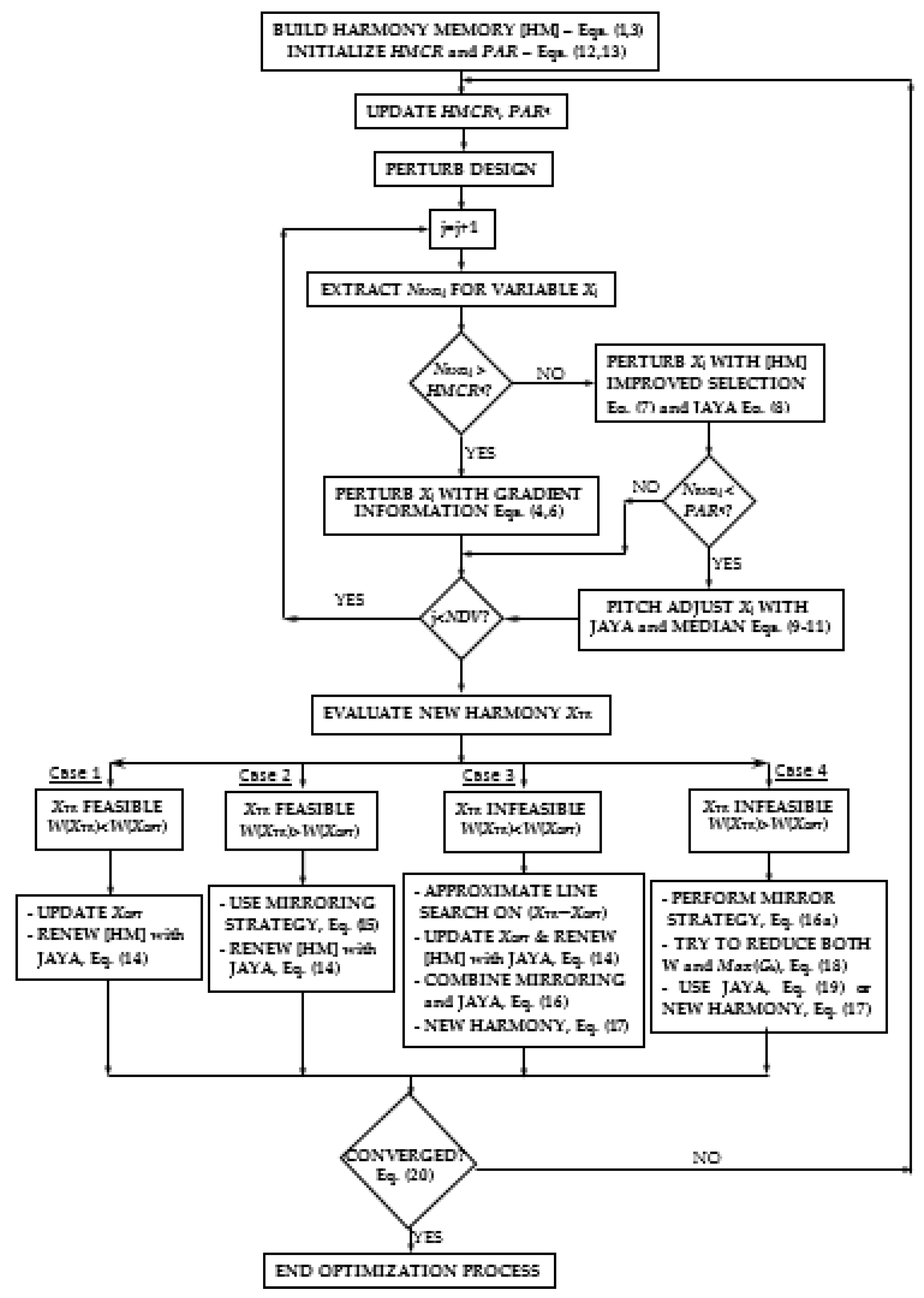
3. The LSSO-HHSJA Algorithm
3.1. Step 1: Generation of New Trial Designs
3.2. Step 2: Evaluation of Trial Design XTR and Population Updating
3.2.1. Case 1: XTR Feasible and W(XTR) < WOPT
3.2.2. Case 2: XTR Feasible but W(XTR) > WOPT
3.2.3. Case 3: XTR Infeasible and W(XTR) < WOPT
3.2.4. Case 4: XTR Infeasible and W(XTR) > WOPT
3.3. Step 3: Check for Convergence
3.4. Step 4: Terminate Optimization Process
4. Test Problems and Optimization Results
4.1. Statement of the Optimization Problem
- xj is the cross-sectional area of the jth element of the truss, included as a sizing design variable, ranging between its lower bound and upper bound ;
- lj is the length of the jth element of the structure;
- g is the gravity acceleration (9.81 m/s2) and ρ is the material density. The g term must not be considered if structural weight is expressed in kg as it was done in the present study;
- u(x,y,z),k,ilc are the displacements of the kth node in the coordinate directions, varying between the lower limit and the upper limit ;
- σj,ilc is the stress in the jth element, varying between (compressive stress limit accounting also for bucking strength) and (allowable tension limit);
- ilc indicates the ilcth loading condition acting on the structure. Constraints on nodal displacements, element stresses and buckling strengths are normalized with respect to their corresponding limits.
4.2. Implementation of the LSSO-HHSJA Algorithm and Comparison with Other Optimizers
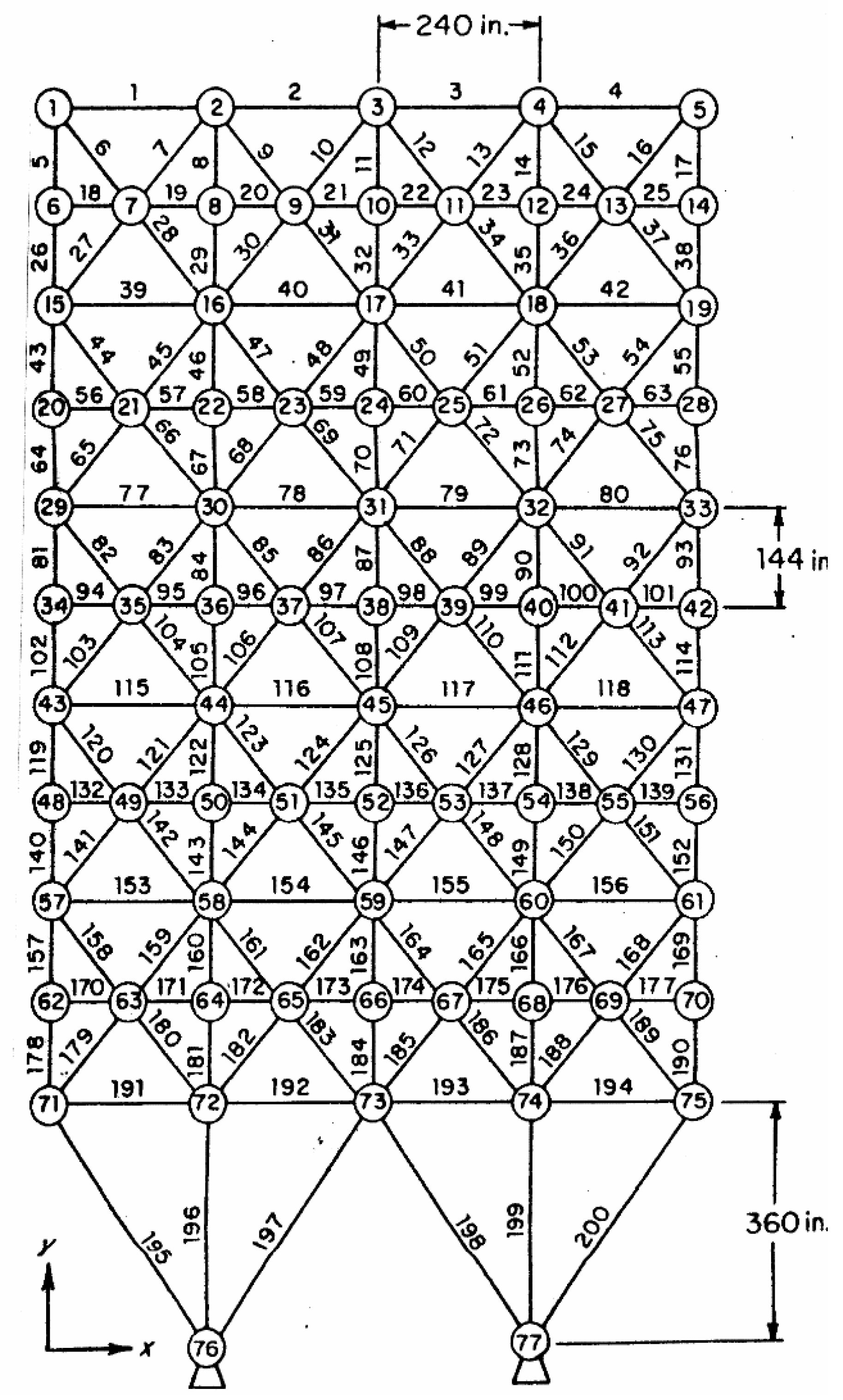
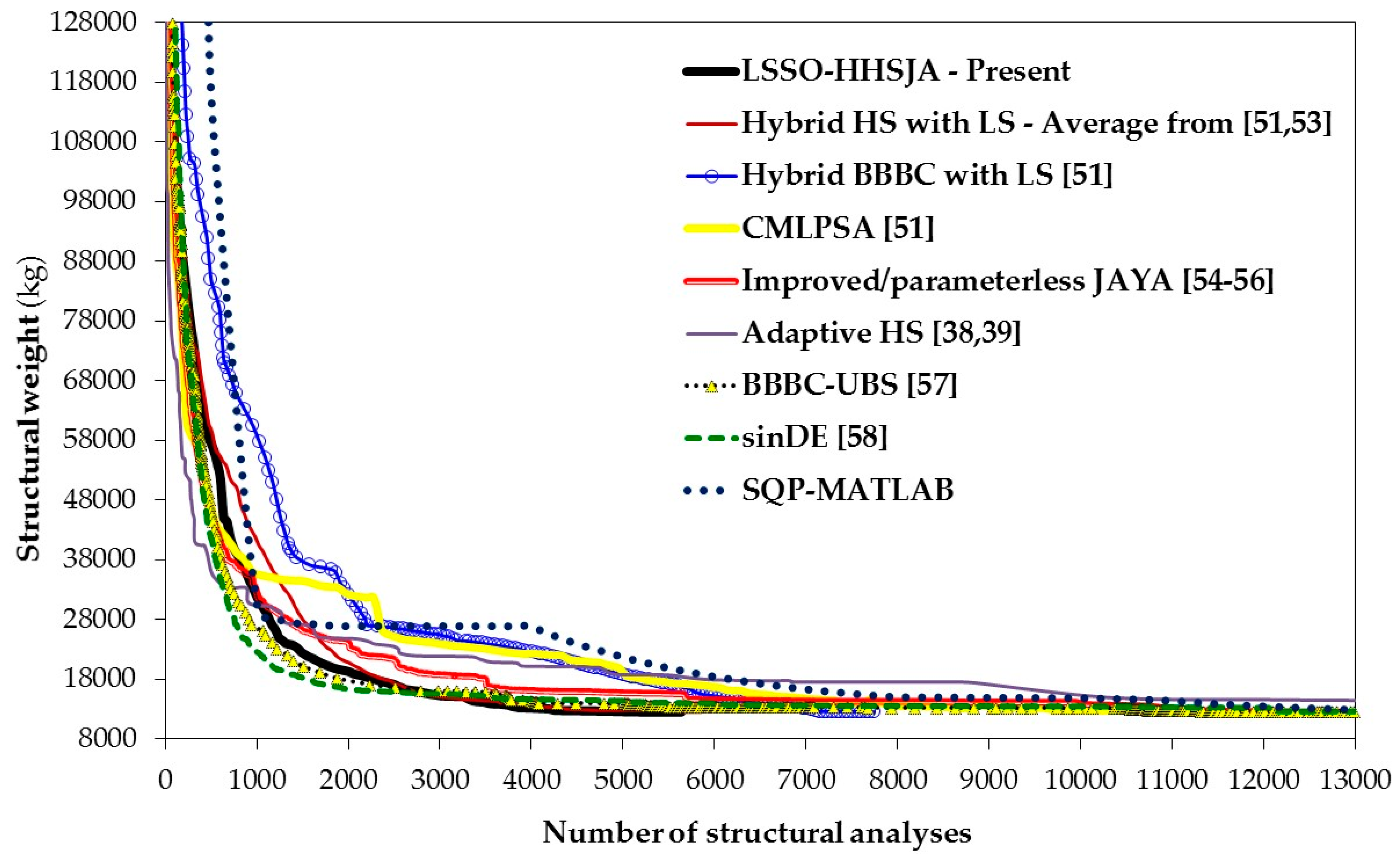
4.3. Planar 200-Bar Truss Structure
- (a)
- 4449.741 N (i.e., 1000 lbf) in the positive X-direction at nodes 1, 6, 15, 20, 29, 34, 43, 48, 57, 62, 71;
- (b)
- 44.497 kN (i.e., 10,000 lbf) in the negative Y-direction at nodes 1, 2, 3, 4, 5, 6, 8, 10, 12, 14, 15, 16, 17, 18, 19, 20, 22, 24, 26, 28, 29, 30, 31, 32, 33, 34, 36, 38, 40, 42, 43, 44, 45, 46, 47, 48, 50, 52, 54, 56, 57, 58, 59, 60, 61, 62, 64, 66, 68, 70, 71, 72, 73, 74, 75;
- (c)
- Loading conditions a) and b) acting together.
- (d)
- 4449.741 N (i.e., 1000 lbf) in the negative X-direction at nodes 5, 14, 19, 28, 33, 42, 47, 56, 61, 70, 75;
- (e)
- Loading conditions (b) and (d) acting together.
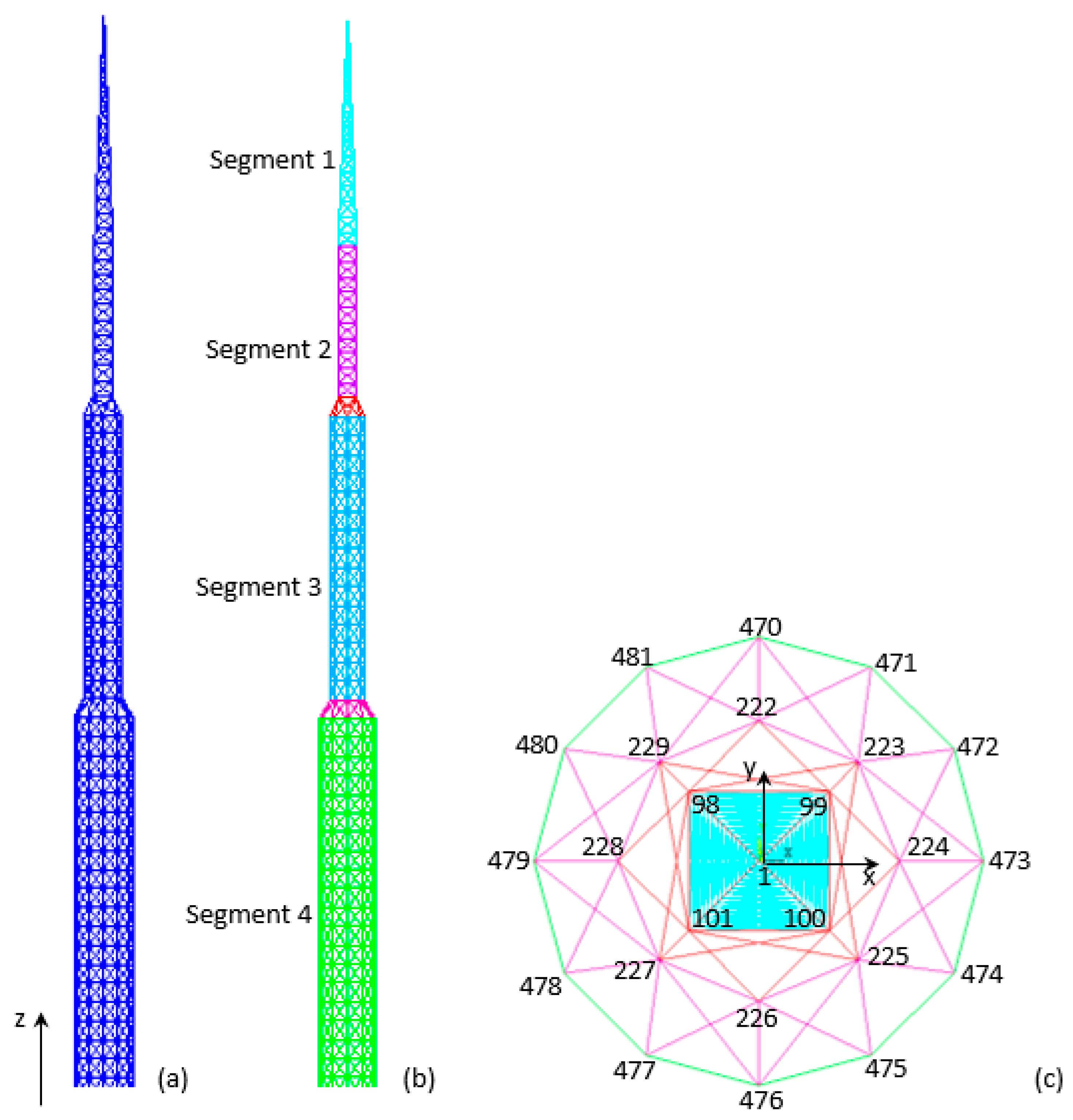
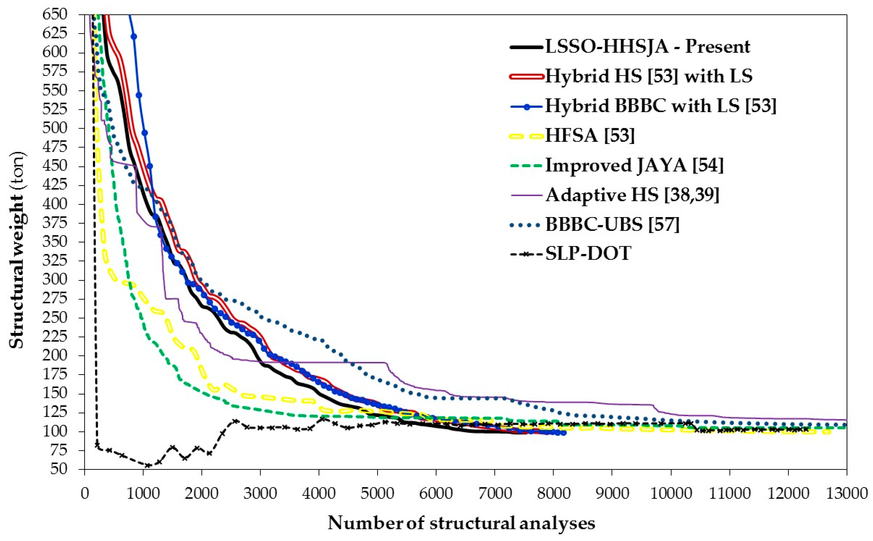
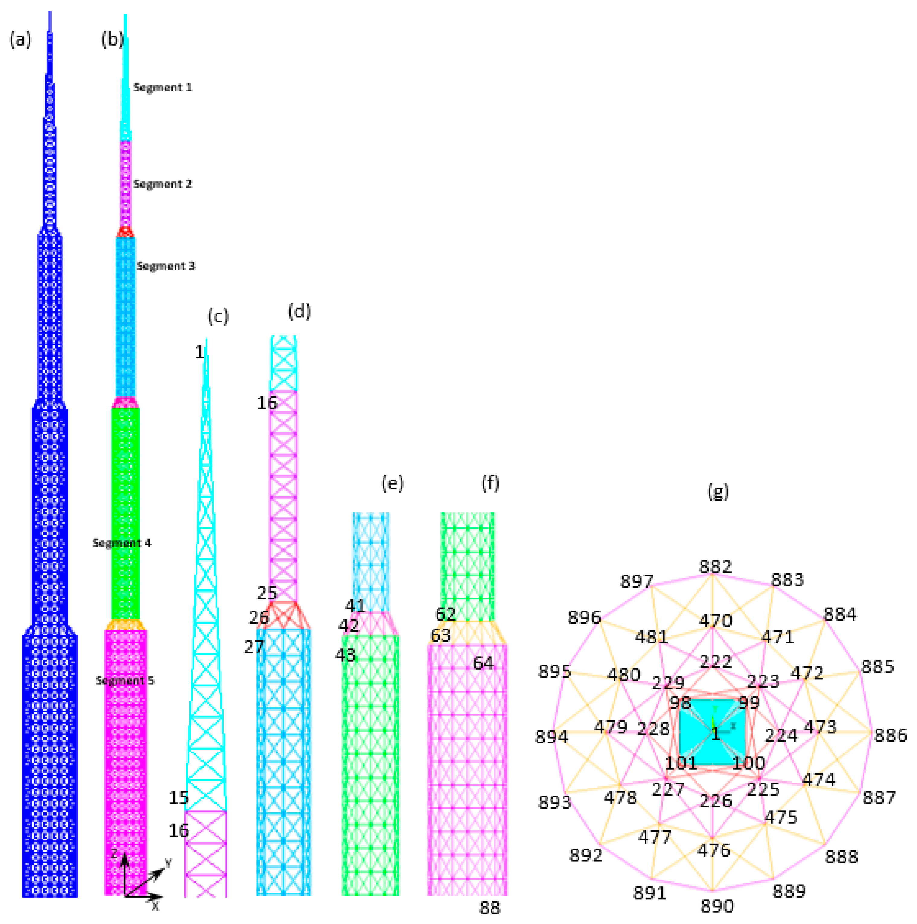
4.4. Spatial 1938-Bar Tower
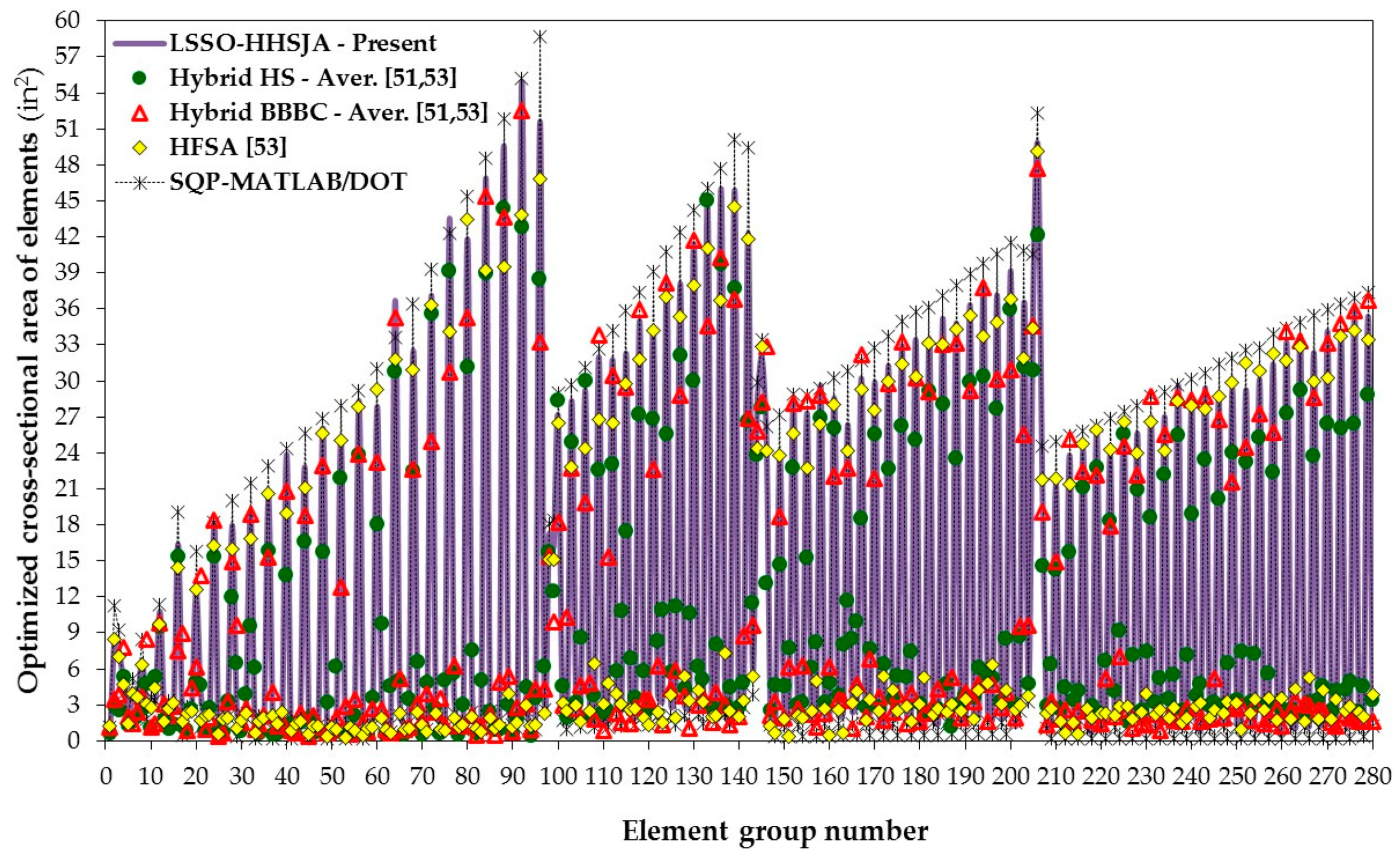
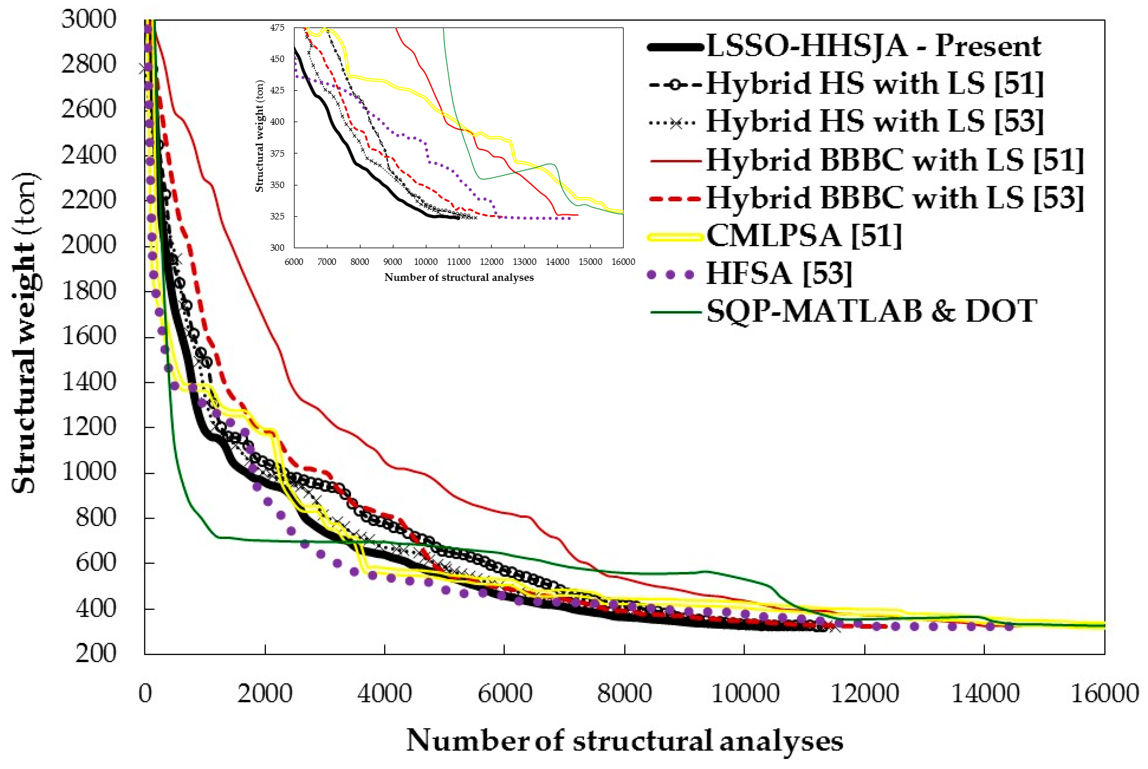
4.5. Spatial 3586-Bar Truss Tower
5. Conclusions
Author Contributions
Funding
Institutional Review Board Statement
Informed Consent Statement
Data Availability Statement
Conflicts of Interest
Appendix A. Details of Geometry for the 1938 and 3586-Bar Towers

| (1) 1–4 | (41) 177–184 | (81) 357–364 | (121) 695–702 | (161) 1231–1242 | (201) 1867–1890 | (241) 2723–2754 |
| (2) 5–6 | (42) 185–186 | (82) 365–366 | (122) 703–718 | (162) 1243–1266 | (202) 1891–1902 | (242) 2755–2770 |
| (3) 7–10 | (43) 187–190 | (83) 367–370 | (123) 719–726 | (163) 1267–1278 | (203) 1903–1914 | (243) 2771–2786 |
| (4) 11–14 | (44) 191–194 | (84) 371–374 | (124) 727–734 | (164) 1279–1290 | (204) 1915–1938 | (244) 2787–2818 |
| (5) 15–22 | (45) 195–202 | (85) 375–382 | (125) 735–750 | (165) 1291–1314 | (205) 1939–1986 | (245) 2819–2834 |
| (6) 23–24 | (46) 203–204 | (86) 383–384 | (126) 751–758 | (166) 1315–1326 | (206) 1987–2002 | (246) 2835–2850 |
| (7) 25–28 | (47) 205–208 | (87) 385–388 | (127) 759–766 | (167) 1327–1338 | (207) 2003–2018 | (247) 2851–2882 |
| (8) 29–32 | (48) 209–212 | (88) 389–392 | (128) 767–782 | (168) 1339–1362 | (208) 2019–2050 | (248) 2883–2898 |
| (9) 33–40 | (49) 213–220 | (89) 393–400 | (129) 783–790 | (169) 1363–1374 | (209) 2051–2066 | (249) 2899–2914 |
| (10) 41–42 | (50) 221–222 | (90) 401–402 | (130) 791–798 | (170) 1375–1386 | (210) 2067–2082 | (250) 2915–2946 |
| (11) 43–46 | (51) 223–226 | (91) 403–406 | (131) 799–814 | (171) 1387–1410 | (211) 2083–2114 | (251) 2947–2962 |
| (12) 47–50 | (52) 227–230 | (92) 407–410 | (132) 815–822 | (172) 1411–1422 | (212) 2115–2130 | (252) 2963–2978 |
| (13) 51–58 | (53) 231–238 | (93) 411–418 | (133) 823–830 | (173) 1423–1434 | (213) 2131–2146 | (253) 2979–3010 |
| (14) 59–60 | (54) 239–240 | (94) 419–420 | (134) 831–846 | (174) 1435–1458 | (214) 2147–2178 | (254) 3011–3026 |
| (15) 61–64 | (55) 241–244 | (95) 421–424 | (135) 847–854 | (175) 1459–1470 | (215) 2179–2194 | (255) 3027–3042 |
| (16) 65–68 | (56) 245–248 | (96) 425–428 | (136) 855–862 | (176) 1471–1482 | (216) 2195–2210 | (256) 3043–3074 |
| (17) 69–76 | (57) 249–256 | (97) 429–436 | (137) 863–878 | (177) 1483–1506 | (217) 2211–2242 | (257) 3075–3090 |
| (18) 77–78 | (58) 257–258 | (98) 437–462 | (138) 879–886 | (178) 1507–1518 | (218) 2243–2258 | (258) 3091–3106 |
| (19) 79–82 | (59) 259–262 | (99) 463–470 | (139) 887–894 | (179) 1519–1530 | (219) 2259–2274 | (259) 3107–3138 |
| (20) 83–86 | (60) 263–266 | (100) 471–478 | (140) 895–910 | (180) 1531–1554 | (220) 2275–2306 | (260) 3139–3154 |
| (21) 87–94 | (61) 267–274 | (101) 479–494 | (141) 911–918 | (181) 1555–1566 | (221) 2307–2322 | (261) 3155–3170 |
| (22) 95–96 | (62) 275–276 | (102) 495–502 | (142) 919–926 | (182) 1567–1578 | (222) 2323–2338 | (262) 3171–3202 |
| (23) 97–100 | (63) 277–280 | (103) 503–510 | (143) 927–942 | (183) 1579–1602 | (223) 2339–2370 | (263) 3203–3218 |
| (24) 101–104 | (64) 281–284 | (104) 511–526 | (144) 943–978 | (184) 1603–1614 | (224) 2371–2386 | (264) 3219–3234 |
| (25) 105–112 | (65) 285–292 | (105) 527–534 | (145) 979–990 | (185) 1615–1626 | (225) 2387–2402 | (265) 3235–3266 |
| (26) 113–114 | (66) 293–294 | (106) 535–542 | (146) 991–1002 | (186) 1627–1650 | (226) 2403–2434 | (266) 3267–3282 |
| (27) 115–118 | (67) 295–298 | (107) 543–558 | (147) 1003–1026 | (187) 1651–1662 | (227) 2435–2450 | (267) 3283–3298 |
| (28) 119–122 | (68) 299–302 | (108) 559–566 | (148) 1027–1038 | (188) 1663–1674 | (228) 2451–2466 | (268) 3299–3330 |
| (29) 123–130 | (69) 303–310 | (109) 567–574 | (149) 1039–1050 | (189) 1675–1698 | (229) 2467–2498 | (269) 3331–3346 |
| (30) 131–132 | (70) 311–312 | (110) 575–590 | (150) 1051–1074 | (190) 1699–1710 | (230) 2499–2514 | (270) 3347–3362 |
| (31) 133–136 | (71) 313–316 | (111) 591–598 | (151) 1075–1086 | (191) 1711–1722 | (231) 2515–2530 | (271) 3363–3394 |
| (32) 137–140 | (72) 317–320 | (112) 599–606 | (152) 1087–1098 | (192) 1723–1746 | (232) 2531–2562 | (272) 3395–3410 |
| (33) 141–148 | (73) 321–328 | (113) 607–622 | (153) 1099–1122 | (193) 1747–1758 | (233) 2563–2578 | (273) 3411–3426 |
| (34) 149–150 | (74) 329–330 | (114) 623–630 | (154) 1123–1134 | (194) 1759–1770 | (234) 2579–2594 | (274) 3427–3458 |
| (35) 151–154 | (75) 331–334 | (115) 631–638 | (155) 1135–1146 | (195) 1771–1794 | (235) 2595–2626 | (275) 3459–3474 |
| (36) 155–158 | (76) 335–338 | (116) 639–654 | (156) 1147–1170 | (196) 1795–1806 | (236) 2627–2642 | (276) 3475–3490 |
| (37) 159–166 | (77) 339–346 | (117) 655–662 | (157) 1171–1182 | (197) 1807–1818 | (237) 2643–2658 | (277) 3491–3522 |
| (38) 167–168 | (78) 347–348 | (118) 663–670 | (158) 1183–1194 | (198) 1819–1842 | (238) 2659–2690 | (278) 3523–3538 |
| (39) 169–172 | (79) 349–352 | (119) 671–686 | (159) 1195–1218 | (199) 1843–1854 | (239) 2691–2706 | (279) 3539–3554 |
| (40) 173–176 | (80) 353–356 | (120) 687–694 | (160) 1219–1230 | (200) 1855–1866 | (240) 2707–2722 | (280) 3555–3586 |

References
- Goldberg, D.E. Genetic Algorithms in Search, Operation and Machine Learning; Addison-Wesley: Boston, MA, USA, 1989. [Google Scholar]
- Storn, R.; Price, K. Differential Evolution—A Simple and Efficient Adaptive Scheme for Global Optimization over Continuous Spaces; Technical Report No. TR-95-012; International Computer Science Institute: Berkley, CA, USA, 1995. [Google Scholar]
- Van Laarhoven, P.J.M.; Aarts, E.H.L. Simulated Annealing: Theory and Applications; Kluwer Academic Publishers: Dordrecht, The Netherlands, 1987. [Google Scholar]
- Clerc, M. Particle Swarm Optimization; ISTE Publishing Company: London, UK, 2006. [Google Scholar]
- Dorigo, M.; Stutzle, T. Ant Colony Optimization; MIT Press: Cambridge, MA, USA, 2004. [Google Scholar]
- Gandomi, A.H.; Yang, X.S.; Alavi, A.H. Mixed variable structural optimization using firefly algorithm. Comput. Struct. 2011, 89, 2325–2336. [Google Scholar] [CrossRef]
- Gandomi, A.H.; Yang, X.S.; Alavi, A.H. Cuckoo search algorithm: A metaheuristic approach to solve structural optimization problems. Eng. Comput. 2013, 29, 17–35. [Google Scholar] [CrossRef]
- Mirjalili, S. The ant lion optimizer. Adv. Eng. Softw. 2015, 83, 80–98. [Google Scholar] [CrossRef]
- Glover, F.; Laguna, M. Tabu Search; Kluwer Academic Publishers: Boston, MA, USA, 1997. [Google Scholar]
- Geem, Z.W.; Kim, J.H.; Loganathan, G. A new heuristic optimization algorithm: Harmony search. Simulation 2001, 76, 60–68. [Google Scholar] [CrossRef]
- Rao, R.V.; Savsani, V.J.; Vakharia, D.P. Teaching–learning-based optimization: A novel method for constrained mechanical design optimization problems. Comput. Aided Des. 2011, 43, 303–315. [Google Scholar] [CrossRef]
- Rao, R.V. Jaya: A simple and new optimization algorithm for solving constrained and unconstrained optimization problems. Int. J. Ind. Eng. Comp. 2016, 7, 19–34. [Google Scholar]
- Erol, O.K.; Eksin, I. A new optimization method: Big bang-big crunch. Adv. Eng. Softw. 2006, 37, 106–111. [Google Scholar] [CrossRef]
- Kaveh, A.; Talatahari, S. A novel heuristic optimization method: Charged system search. Acta Mech. 2010, 213, 267–289. [Google Scholar] [CrossRef]
- Kaveh, A.; Khayat Azad, M. A new meta-heuristic method: Ray optimization. Comput. Struct. 2012, 112–113, 283–294. [Google Scholar] [CrossRef]
- Kaveh, A.; Mahdavi, V.R. Colliding bodies optimization: A novel meta-heuristic method. Comput. Struct. 2014, 139, 18–27. [Google Scholar] [CrossRef]
- Kaveh, A.; Bakhshpoori, T. A new metaheuristic for continuous structural optimization: Water evaporation optimization. Struct. Multidiscip. Optim. 2016, 54, 23–43. [Google Scholar] [CrossRef]
- Kaveh, A.; Zolghadr, A. Cyclical parthenogenesis algorithm for guided modal strain energy based structural damage detection. Appl. Soft Comput. 2017, 57, 250–264. [Google Scholar] [CrossRef]
- Pierezan, J.; Coelho, L.S. Coyote optimization algorithm: A new metaheuristic for global optimization problems. In Proceedings of the IEEE World Conference on Computational Intelligence, Congress on Evolutionary Computation, Rio de Janeiro, Brazil, 8–13 July 2018; pp. 2633–2640. [Google Scholar]
- Lamberti, L.; Pappalettere, C. Metaheuristic design optimization of skeletal structures: A review. Comput. Technol. Rev. 2011, 4, 1–32. [Google Scholar] [CrossRef]
- Saka, M.P.; Dogan, E. Recent developments in metaheuristic algorithms: A review. Comput. Technol. Rev. 2012, 5, 31–78. [Google Scholar] [CrossRef]
- Kaveh, A. Advances in Metaheuristic Algorithms for Optimal Design of Structures; Springer International Publishing: Cham, Switzerland, 2014. [Google Scholar]
- Kaveh, A. Applications of Metaheuristic Optimization Algorithms in Civil Engineering; Springer International Publishing: Cham, Switzerland, 2017. [Google Scholar]
- Kaveh, A.; Ilchi Ghazaan, M. Meta-Heuristic Algorithms for Optimal Design of Real-Size Structures; Springer International Publishing: Cham, Switzerland, 2018. [Google Scholar]
- Wolpert, D.H.; Macready, W.G. No Free Lunch Theorems for optimization. IEEE Trans. Evol. Comput. 1997, 1, 67–82. [Google Scholar] [CrossRef]
- Ho, Y.C.; Pepyne, D.L. Simple explanation of the No-Free-Lunch Theorem and its implications. J. Optim. Theory Appl. 2002, 115, 549–570. [Google Scholar] [CrossRef]
- Yang, X.-S. Harmony search as a metaheuristic algorithm. In Music-Inspired Harmony Search Algorithm: Theory and Applications; Geem, Z.W., Ed.; Springer: Berlin/Heidelberg, Germany, 2009; pp. 1–14. [Google Scholar]
- Haftka, R.T.; Gurdal, Z. Elements of Structural Optimization, 3rd ed.; Kluwer Academic Publishers: Dordrecht, The Netherlands, 1992. [Google Scholar]
- Vanderplaats, G.N. Numerical Optimization Techniques for Engineering Design; VR&D Inc.: Colorado Springs, CO, USA, 1998. [Google Scholar]
- Arora, J.S. Introduction to Optimum Design; McGraw-Hill Book Company: New York, NY, USA, 1989. [Google Scholar]
- Lee, K.S.; Geem, Z.W. A new structural optimization method based on the harmony search algorithm. Comput. Struct. 2004, 82, 781–798. [Google Scholar] [CrossRef]
- Lee, K.S.; Geem, Z.W. A new meta-heuristic algorithm for continuous engineering optimization: Harmony search theory and practice. Comput. Methods Appl. Mech. Eng. 2005, 194, 3902–3933. [Google Scholar] [CrossRef]
- Saka, M.P. Optimum design of steel sway frames to BS5950 using harmony search algorithm. J. Constr. Steel Res. 2009, 65, 36–43. [Google Scholar] [CrossRef]
- Maheri, M.R.; Narimani, M.N. An enhanced harmony search algorithm for optimum design of side sway steel frames. Comput. Struct. 2014, 136, 78–89. [Google Scholar] [CrossRef]
- Murren, P.; Khandelwal, K. Design-driven harmony search (DDHS) in steel frame optimization. Eng. Struct. 2014, 59, 798–808. [Google Scholar] [CrossRef]
- Mahdavi, M.; Fesanghary, M.; Damangir, E. An improved harmony search algorithm for solving optimization problems. Appl. Math. Comput. 2007, 188, 1567–1579. [Google Scholar] [CrossRef]
- Carbas, S.; Saka, M.P. Optimum topology design of various geometrically nonlinear latticed domes using improved harmony search method. Struct. Multidiscip. Optim. 2012, 45, 377–399. [Google Scholar] [CrossRef]
- Hasancebi, O.; Erdal, F.; Saka, M.P. Adaptive harmony search method for structural optimization. ASCE J. Struct. Eng. 2010, 136, 419–431. [Google Scholar] [CrossRef]
- Degertekin, S.O. Improved harmony search algorithms for sizing optimization of truss structures. Comput. Struct. 2012, 92–93, 229–241. [Google Scholar] [CrossRef]
- Kaveh, A.; Naiemi, M. Sizing optimization of skeletal structures with a multi-adaptive Harmony Search algorithm. Sci. Iran. Trans. Civil Eng. 2015, 22, 345–366. [Google Scholar]
- Geem, Z.W.; Sim, K.B. Parameter-setting-free harmony search algorithm. Appl. Math. Comput. 2010, 217, 3881–3889. [Google Scholar] [CrossRef]
- Turky, A.M.; Abdullah, S. A multi-population harmony search algorithm with external archive for dynamic optimization problems. Inform. Sci. 2014, 272, 84–95. [Google Scholar] [CrossRef]
- Kaveh, A.; Ahangaran, M. Discrete cost optimization of composite floor system using social harmony search model. Appl. Soft Comput. 2012, 12, 372–381. [Google Scholar] [CrossRef]
- Cheng, M.Y.; Prayogo, D.; Wu, Y.W.; Lukito, M.M. A Hybrid Harmony Search algorithm for discrete sizing optimization of truss structure. Auto. Constr. 2016, 69, 21–33. [Google Scholar] [CrossRef]
- Kaveh, A.; Talatahari, S. A particle swarm ant colony optimization for truss structures with discrete variables. J. Constr. Steel Res. 2009, 65, 1558–1568. [Google Scholar] [CrossRef]
- Kaveh, A.; Talatahari, S. Particle swarm optimizer, ant colony strategy and harmony search scheme hybridized for optimization of truss structures. Comput. Struct. 2009, 87, 267–283. [Google Scholar] [CrossRef]
- Omran, M.G.H.; Mahdavi, M. Global best harmony search. Appl. Math. Comput. 2008, 198, 643–656. [Google Scholar] [CrossRef]
- Al-Betar, M.A.; Abu Doush, I.; Khader, A.T.; Awadallah, M.A. Novel selection schemes for harmony search. Appl. Math. Comput. 2012, 218, 6095–6117. [Google Scholar] [CrossRef]
- Fesanghary, M.; Mahdavi, M.; Minary-Jolandan, M.; Alizadeh, Y. Hybridizing harmony search algorithm with sequential quadratic programming for engineering optimization problems. Comput. Methods Appl. Mech. Eng. 2008, 197, 3080–3091. [Google Scholar] [CrossRef]
- Lamberti, L.; Pappalettere, C. An improved harmony-search algorithm for truss structure optimization. In Proceedings of the Twelfth International Conference on Civil, Structural and Environmental Engineering Computing, Funchal, Portugal, 1–4 September 2009; Topping, B.H.V., Costa Neves, L.F., Barros, R.C., Eds.; [Google Scholar]
- Lamberti, L.; Pappalettere, C. Truss weight minimization using hybrid Harmony Search and Big Bang-Big Crunch algorithms. In Metaheuristic Applications in Structures and Infrastructures; Gandomi, A.H., Yang, X.S., Talatahari, S., Alavi, A.H., Eds.; Elsevier: Waltham, MA, USA, 2013; pp. 207–240. [Google Scholar]
- Degertekin, S.O.; Lamberti, L. Comparison of hybrid metaheuristic algorithms for truss weight optimization. In Proceedings of the Third International Conference on Soft Computing Technology in Civil, Structural and Environmental Engineering, Cagliari, Italy, 3–6 September 2013; Tsompanakis, Y., Ed.; [Google Scholar]
- Ficarella, E.; Lamberti, L.; Degertekin, S.O. Comparison of three novel hybrid metaheuristic algorithms for structural optimization problems. Comput. Struct. 2021, 244, 106395. [Google Scholar] [CrossRef]
- Degertekin, S.O.; Lamberti, L.; Ugur, I.B. Sizing, layout and topology design optimization of truss structures using the Jaya algorithm. Appl. Soft Comput. 2018, 70, 903–928. [Google Scholar] [CrossRef]
- Degertekin, S.O.; Lamberti, L.; Ugur, I.B. Discrete sizing/layout/topology optimization of truss structures with an advanced Jaya algorithm. Appl. Soft Comput. 2019, 79, 363–390. [Google Scholar] [CrossRef]
- Degertekin, S.O.; Yalcin Bayar, G.; Lamberti, L. Parameter free Jaya algorithm for truss sizing-layout optimization under natural frequency constraints. Comput. Struct. 2021, 245, 106461. [Google Scholar] [CrossRef]
- Kazemzadeh Azad, S.; Hasancebi, O.; Kazemzadeh Azad, S.; Erol, O.K. Upper bound strategy in optimum design of truss structures: A big bang-big crunch algorithm based application. Adv. Struct. Eng. 2013, 16, 1035–1046. [Google Scholar] [CrossRef]
- Draa, A.; Bouzoubia, S.; Boukhalfa, I. A sinusoidal differential evolution algorithm for numerical optimization. Appl. Soft Comput. 2015, 27, 99–126. [Google Scholar] [CrossRef]
- The MathWorks. MATLAB® Release 2018b; The MathWorks: Austin, TX, USA, 2018. [Google Scholar]
- Vanderplaats, G.N. DOTs Users Manual, Version 4.20; VR&D Inc.: Colorado Springs, CO, USA, 1995. [Google Scholar]


| NPOP | Structural Weight (kg) | Structural Analyses | Constraint Tolerance (%) |
|---|---|---|---|
| 20 | 12,483.673 | 5562 | Feasible |
| 12,490.377 * | 5668 * | 0.00735 * | |
| 12,489.460 ♦ | 5716 ♦ | 0.003451 ♦ | |
| 50 | 12,483.563 | 5734 | Feasible |
| 12,490.482 * | 6604 * | 0.00750 * | |
| 12,489.457 ♦ | 6040 ♦ | 0.003250 ♦ | |
| 100 | 12,484.135 | 6096 | Feasible |
| 12,490.542 * | 6360 * | 0.00750 * | |
| 12,489.778 ♦ | 5621 ♦ | 0.002802 ♦ | |
| 200 | 12,483.982 | 5436 | Feasible |
| 12,490.332 * | 5679 * | 0.00730 * | |
| 12,489.700 ♦ | 5831 ♦ | 0.003168 ♦ | |
| 500 | 12,483.339 | 5637 | Feasible |
| 12,490.414* | 5940 * | 0.00643 * | |
| 12,489.619 ♦ | 6372 ♦ | 0.003524 ♦ | |
| 1000 | 12,484.054 | 6373 | Feasible |
| 12,490.427* | 5938 * | 0.00560 * | |
| 12,489.564 ♦ | 6217 ♦ | 0.003329 ♦ |
| Optimized Weight (kg) | Number of Structural Analyses | Constraint Violation (%) | |
|---|---|---|---|
| LSSO-HHSJA Present | Best: 12,483.339 | Best: 5637 | |
| Worst: 12,484.135 | Fastest: 5436 | Feasible | |
| Mean: 12,483.791 | Slowest: 6373 | ||
| STD: 0.3144 | Mean/STD: 5806 ± 357 | ||
| Hybrid HS with LS [51] | Best: 12,490.332 | Best: 5679 | Best: 0.00730 |
| Worst: 12,490.542 | Fastest: 5668 | Worst: 0.00750 | |
| Mean: 12,490.430 | Slowest: 6604 | Mean: 0.00695 | |
| STD: 0.07470 | Mean/STD: 6031 ± 377 | STD: 0.000772 | |
| Hybrid HS with LS [53] | Best: 12,489.457 | Best: 6040 | Best: 0.003250 |
| Worst: 12,489.778 | Fastest: 5621 | Worst: 0.002802 | |
| Mean: 12,489.596 | Slowest: 6372 | Mean: 0.003254 | |
| STD: 0.1291 | Mean/STD: 5966 ± 324 | STD: 0.0002565 | |
| Hybrid BBBC with LS [51] | Best: 12,490.439 | Best: 7745 | Best: 0.00559 |
| Worst: 12,490.932 | Fastest: 1924 | Worst: 0.00625 | |
| Mean: 12,490.680 | Slowest: 9460 | Mean: 0.00626 | |
| STD: 0.1773 | Mean/STD: 5652 ± 2912 | STD: 0.000347 | |
| CMLPSA [51] | Best: 12,492.888 | Best: 11,726 | |
| Worst: 12,493.290 | Fastest: 10,338 | Feasible | |
| Mean: 12,493.081 | Slowest: 12,118 | ||
| STD: 0.2014 | Mean/STD: 11,394 ± 935 | ||
| Improved/parameterless JAYA [54,55,56] | Best: 12,490.603 | Best: 12,869 | Best: 0.03490 |
| Worst: 12,502.175 | Fastest: 12,316 | Worst: Feasible | |
| Mean: 12,494.460 | Slowest: 14,326 | Mean: 0.01888 | |
| STD: 3.056 | Mean/STD: 12,818 ± 601 | STD: 0.01644 | |
| AHS [38] | Best: 12,497.475 | Best: 16,981 | Best: 0.1570 |
| Worst: 12,777.339 | Fastest: 15,063 | Worst: Feasible | |
| Mean: 12,567.441 | Slowest: 21,412 | Mean: 0.08363 | |
| STD: 174.716 | Mean/STD: 17,130 ± 2996 | STD: 0.06836 | |
| SAHS [39] | Best: 12,495.939 | Best: 15,812 | Best: 0.1824 |
| Worst: 12,669.384 | Fastest: 13,384 | Worst: Feasible | |
| Mean: 12,553.754 | Slowest: 17,464 | Mean: 0.09718 | |
| STD: 144.817 | Mean/STD: 15,618 ± 1681 | STD: 0.07942 | |
| BBBC-UBS [57] | Best: 12,490.035 | Best: 15,250 | Best: 0.05540 |
| Worst: 12,502.346 | Fastest: 13,865 | Worst: Feasible | |
| Mean: 12,497.562 | Slowest: 16,198 | Mean: 0.03048 | |
| STD: 4.170 | Mean/STD: 14,795 ± 1141 | STD: 0.02837 | |
| sinDE [58] | Best: 12,502.536 | Best: 21,653 | Best: 0.05880 |
| Worst: 12,541.640 | Fastest: 17,124 | Worst: Feasible | |
| Mean: 12,520.999 | Slowest: 22,635 | Mean: 0.03030 | |
| STD: 16.369 | Mean/STD: 20,766 ± 2472 | STD: 0.03017 | |
| SQP-MATLAB | Best: 12,491.400 | Best: 28,198 | Best: 0.05131 |
| Worst: 12,503.300 | Fastest: 24,619 | Worst: Feasible | |
| Mean: 12,498.034 | Slowest: 38,410 | Mean: 0.03298 | |
| STD: 5.661 | Mean/STD: 30,990 ± 5957 | STD: 0.03969 |
| Loading Condition 1 | |
| X | None |
| Y | None |
| Z | −13.5 kN @ nodes 1 through 61 (the “–“ sign indicates that concentrated forces act in the negative Z-direction); −27 kN @ nodes 62 through 101; −40.5 kN @ nodes 102 through 229; −54 kN @ nodes 230 through 469. |
| Loading condition 2 | |
| X | +6.672 kN @ nodes 2, 5, 6, 9, 10, 13, 14, 17, 18, 21, 22, 25, 26, 29, 30, 33, 34, 37, 38, 41, 42, 45, 46, 49, 50, 53, 54, 57, 58, 61, 62, 65, 66, 69, 70, 81, 82, 85, 86, 89, 90, 93, 94, 97, 98, 101, 108, 116, 124, 132, 140, 148, 156, 164, 172, 180, 188, 196, 204, 220, 228, 239, 251, 263, 275, 287, 299, 311, 323, 335, 347, 359, 371, 383, 395, 407, 419, 431, 443, 455, 467; −4.448 kN @ nodes 3, 4, 7, 8, 11, 12, 15, 16, 19, 20, 23, 24, 27, 28, 31, 32, 35, 36, 39, 40, 43, 44, 47, 48, 51, 52, 55, 56, 59,60, 63, 64, 67, 68, 71, 72, 75, 76, 79, 80, 83, 84, 87, 88, 91, 92, 95, 96, 99, 100, 104, 112, 120, 128, 136, 144, 152, 160, 168, 176, 184, 192, 200, 208, 216, 224, 233, 245, 257, 269, 281, 293, 305, 317, 329, 341, 353, 365, 377, 389, 401, 413, 425, 437, 449, 461 (the “–“ sign indicates that concentrated forces act in the negative X-direction). |
| Y | None |
| Z | None |
| Loading condition 3 | |
| X | None |
| Y | −4.448 kN @ nodes 2, 3, 6, 7, 10, 11, 14, 15, 18, 19, 22, 23, 26, 27, 30, 31, 34, 35, 38, 39, 42, 43, 46, 47, 50, 51, 54, 55, 58, 59, 62, 63, 66, 67, 70, 71, 74, 75, 78, 79, 82, 83, 86, 87, 90, 91, 94, 95, 98, 99, 102, 110, 118, 126, 134, 142, 150, 158, 166, 174, 182, 190, 198, 206, 214, 222, 230, 242, 266, 278, 290, 302, 314, 326, 338, 350, 362, 374, 386, 398, 410, 422, 434, 446, 458 (the “–“ sign indicates that concentrated forces act in the negative Y-direction); +4.448 kN @ nodes 4, 5, 8, 9, 12, 13, 16, 17, 20, 21, 24, 25, 28, 29, 32, 33, 36, 37, 40, 41, 44, 45, 48, 49, 52, 53, 56, 57, 60, 61, 64, 65, 68, 69, 72, 73, 76, 77, 80, 81, 84, 85, 88, 89, 92, 93, 96, 97, 100, 101, 106, 114, 122, 130, 138, 146, 154, 162, 170, 178, 186, 194, 202, 210, 218, 226, 236, 248, 260, 272, 284, 296, 308, 320, 332, 344, 356, 368, 380, 392, 404, 416, 428, 440, 452, 464. |
| Z | None |
| Optimized Weight (ton) | Number of Structural Analyses | Constraint Violation (%) | |
|---|---|---|---|
| LSSO-JAYA Present | Best: 98.822 | Best: 7529 | Feasible |
| Worst: 98.860 | Worst: 7780 | ||
| Mean/STD: 98.832 ± 0.01980 | Mean/STD: 7680 ± 284 | ||
| Hybrid HS with LS [53] | Best: 100.008 | Best: 7931 | Feasible |
| Worst: 100.240 | Worst: 8694 | ||
| Mean/STD: 100.147 ± 0.467 | Mean/STD: 8395 ± 657 | ||
| Hybrid BBBC with LS [53] | Best: 99.164 | Best: 8167 | Feasible |
| Worst: 99.225 | Worst: 9655 | ||
| Mean/STD: 99.179 ± 0.02687 | Mean/STD: 8861 ± 526 | ||
| HFSA [53] | Best: 99.794 | Feasible | |
| Worst: 101.251 | 13201 ± 598 | ||
| Mean/STD: 100.523 ± 0.516 | |||
| Improved JA [54] | Best: 99.255 | Best: 20,051 | Feasible |
| Worst: 99.265 | Worst: 21,980 | ||
| Mean/STD: 99.263 ± 0.003536 | Mean/STD: 21,136 ± 843 | ||
| AHS [38] | Best: 100.750 | Best: 19,139 | Feasible |
| Worst: 103.421 | Worst: 17,184 | ||
| Mean/STD: 101.919 ± 1.653 | Mean/STD: 18,394 ± 1134 | ||
| SAHS [39] | Best: 100.120 | Best: 15,437 | Feasible |
| Worst: 104.368 | Worst: 14,297 | ||
| Mean/STD: 102.623 ± 2.188 | Mean/STD: 15,201 ± 1383 | ||
| BBBC-UBS [57] | Best: 101.120 | Best: 17,461 | Feasible |
| Worst: 102.628 | Worst: 19,980 | ||
| Mean/STD: 101.335 ± 0.3033 | Mean/STD: 18,930 ± 666 | ||
| SLP-DOT | 102.789 | 12,310 | Feasible |
| Loading Condition 1 | |
| X | None |
| Y | None |
| Z | −13.5 kN @ nodes 1 through 61 (the “–“ sign indicates that concentrated forces act in the negative Z-direction); −27 kN @ nodes 62 through 101; −40.5 kN @ nodes 102 through 229; −54 kN @ nodes 230 through 481; −67.5 kN @ nodes 482 through 881. |
| Loading condition 2 | |
| X | +6.672 kN @ nodes 2, 5, 6, 9, 10, 13, 14, 17, 18, 21, 22, 25, 26, 29, 30, 33, 34, 37, 38, 41, 42, 45, 46, 49, 50, 53, 54, 57, 58, 61, 62, 65, 66, 69, 70, 81, 82, 85, 86, 89, 90, 93, 94, 97, 98, 101, 108, 116, 124, 132, 140, 148, 156, 164, 172, 180, 188, 196, 204, 220, 228, 239, 251, 263, 275, 287, 299, 311, 323, 335, 347, 359, 371, 383, 395, 407, 419, 431, 443, 455, 467, 479, 494, 510, 526, 542, 558, 574, 590, 606, 622, 638, 654, 670, 686, 702, 718, 734, 750, 766, 782, 798, 814, 830, 846, 862, 878; −4.448 kN @ nodes 3, 4, 7, 8, 11, 12, 15, 16, 19, 20, 23, 24, 27, 28, 31, 32, 35, 36, 39, 40, 43, 44, 47, 48, 51, 52, 55, 56, 59, 60, 63, 64, 67, 68, 71, 72, 75, 76, 79, 80, 83, 84, 87, 88, 91, 92, 95, 96, 99, 100, 104, 112, 120, 128, 136, 144, 152, 160, 168, 176, 184, 192, 200, 208, 216, 224, 233, 245, 257, 269, 281, 293, 305, 317, 329, 341, 353, 365, 377, 389, 401, 413, 425, 437, 449, 461, 473, 486, 502, 518, 534, 550, 566, 582, 598, 606, 622, 638, 654, 670, 686, 702, 718, 734, 750, 766, 782, 798, 814, 830, 846, 862, 878 (the “–“ sign indicates that concentrated forces act in the negative X-direction). |
| Y | None |
| Z | None |
| Loading condition 3 | |
| X | None |
| Y | −4.448 kN @ nodes 2, 3, 6, 7, 10, 11, 14, 15, 18, 19, 22, 23, 26, 27, 30, 31, 34, 35, 38, 39, 42, 43, 46, 47, 50, 51, 54, 55, 58, 59, 62, 63, 66, 67, 70, 71, 74, 75, 78, 79, 82, 83, 86, 87, 90, 91, 94, 95, 98, 99, 102, 110, 118, 126, 134, 142, 150, 158, 166, 174, 182, 190, 198, 206, 214, 222, 230, 242, 266, 278, 290, 302, 314, 326, 338, 350, 362, 374, 386, 398, 410, 422, 434, 446, 458, 470, 482, 498, 514, 530, 546, 562, 578, 594, 610, 626, 642, 658, 674, 690, 706, 722, 738, 754, 770, 786, 802, 818, 834, 850, 866 (the “–“ sign indicates that concentrated forces act in the negative Y-direction); +4.448 kN @ nodes 4, 5, 8, 9, 12, 13, 16, 17, 20, 21, 24, 25, 28, 29, 32, 33, 36, 37, 40, 41, 44, 45, 48, 49, 52, 53, 56, 57, 60, 61, 64, 65, 68, 69, 72, 73, 76, 77, 80, 81, 84, 85, 88, 89, 92, 93, 96, 97, 100, 101, 106, 114, 122, 130, 138, 146, 154, 162, 170, 178, 186, 194, 202, 210, 218, 226, 236, 248, 260, 272, 284, 296, 308, 320, 332, 344, 356, 368, 380, 392, 404, 416, 428, 440, 452, 464, 476, 490, 506, 522, 538, 554, 570, 586, 602, 618, 634, 650, 666, 682, 698, 714, 730, 746, 762, 778, 794, 810, 826, 842, 858, 874. |
| Z | None |
| Optimized Weight (ton) | Number of Structural Analyses | Constraint Violation (%) | |
|---|---|---|---|
| LSSO-JAYA Present | Best: 323.175 | Best: 10,997 | Feasible |
| Worst: 323.722 | Worst: 11,753 | ||
| Mean/STD: 323.287 ± 0.158 | Mean/STD: 11,262 ± 534 | ||
| Hybrid HS with LS [51] | 325.381 | 11,312 | 0.06110 |
| Hybrid HS with LS [53] | Best: 323.611 | Best: 11,504 | Best: 0.03679 |
| Worst: 324.794 | Worst: 12,046 | Worst: 0.02170 | |
| Mean/STD: 324.202 ± 0.4358 | Mean/STD: 11,904 ± 628 | Mean/STD: 0.0317 ± 0.00986 | |
| Hybrid BBBC with LS [51] | 325.980 | 14,616 | 0.06180 |
| Hybrid BBBC with LS [53] | Best: 324.246 | Best: 12,356 | Best: 0.02376 |
| Worst: 325.752 | Worst: 13,403 | Worst: 0.03750 | |
| Mean/STD: 325.299 ± 0.5607 | Mean/STD: 13,295 ± 789 | Mean/STD: 0.0269 ± 0.0104 | |
| CMLPSA [51] | 326.185 | 16,240 | 0.105 |
| HFSA [53] | Best: 323.567 | Feasible | |
| Worst: 325.329 | 14,466 ± 565 | ||
| Mean/STD: 324.385 ± 0.4283 | |||
| Improved/parameterless JA [54,55,56] | Best: 323.977 | Feasible | |
| Worst: 324.431 | Computational budget: 20,000 structural analyses | ||
| Mean/STD: 324.130 ± 0.287 | |||
| BBBC-UBS [57] | Best: 325.097 | Feasible | |
| Worst: 327.681 | Computational budget: 20,000 structural analyses | ||
| Mean/STD: 325.541 ± 1.083 | |||
| SLP-MATLAB & DOT | 326.278 | 16,480 | Feasible |
Publisher’s Note: MDPI stays neutral with regard to jurisdictional claims in published maps and institutional affiliations. |
© 2021 by the authors. Licensee MDPI, Basel, Switzerland. This article is an open access article distributed under the terms and conditions of the Creative Commons Attribution (CC BY) license (https://creativecommons.org/licenses/by/4.0/).
Share and Cite
Degertekin, S.O.; Minooei, M.; Santoro, L.; Trentadue, B.; Lamberti, L. Large-Scale Truss-Sizing Optimization with Enhanced Hybrid HS Algorithm. Appl. Sci. 2021, 11, 3270. https://doi.org/10.3390/app11073270
Degertekin SO, Minooei M, Santoro L, Trentadue B, Lamberti L. Large-Scale Truss-Sizing Optimization with Enhanced Hybrid HS Algorithm. Applied Sciences. 2021; 11(7):3270. https://doi.org/10.3390/app11073270
Chicago/Turabian StyleDegertekin, Sadik Ozgur, Mohammad Minooei, Lorenzo Santoro, Bartolomeo Trentadue, and Luciano Lamberti. 2021. "Large-Scale Truss-Sizing Optimization with Enhanced Hybrid HS Algorithm" Applied Sciences 11, no. 7: 3270. https://doi.org/10.3390/app11073270
APA StyleDegertekin, S. O., Minooei, M., Santoro, L., Trentadue, B., & Lamberti, L. (2021). Large-Scale Truss-Sizing Optimization with Enhanced Hybrid HS Algorithm. Applied Sciences, 11(7), 3270. https://doi.org/10.3390/app11073270