Article

EPTlib: An Open-Source Extensible Collection of Electric Properties Tomography Techniques

by
Alessandro Arduino
Istituto Nazionale di Ricerca Metrologica (INRiM), 10135 Torino, Italy
Appl. Sci. 2021, 11(7), 3237; https://doi.org/10.3390/app11073237
Submission received: 27 February 2021 / Revised: 31 March 2021 / Accepted: 1 April 2021 / Published: 4 April 2021
(This article belongs to the Special Issue Latest Advances and Applications of Magnetic Resonance Imaging)

Abstract

:

Featured Application

EPTlib is an ongoing project for an open-source extensible C++ library collecting electric properties tomography techniques. It is freely distributed and includes a terminal application for a simple ready-to-use adoption of the implemented techniques.

Abstract

Electric properties tomography (EPT) is a novel magnetic resonance imaging–based method to estimate non-invasively the distribution of the electric properties in the human body. In this paper, EPTlib, an open-source extensible C++ library collecting ready-to-use algorithms for electric properties tomography, is presented. Currently, EPTlib implements three techniques, named Helmholtz-EPT, convection-reaction-EPT and gradient-EPT, whose derivation and implementation is deeply discussed. Moreover, the configuration files needed by the terminal application included in EPTlib to apply the implemented techniques are outlined. The three techniques are applied to a couple of model problems in order to highlight their main features and the effects of the tunable parameters.

1. Introduction

Traditional magnetic resonance imaging (MRI) produces qualitative images that are weighted according to certain physical and operative parameters. The interpretation of these images is based only on the relative contrast between pixels of the same image and the comparison of the results of acquisitions conducted with different scanners or at different times is not straightforward, because of the lack of a common reference. Quantitative MRI, namely an MRI process that produces images which are pixel-by-pixel measurements of a physical quantity, is arousing increasing interest, because it would overcome the mentioned intercomparison issue. Examples of MRI-based quantitative imaging are magnetic resonance fingerprinting [1], which provides an estimate of the distribution of the relaxation times T 1 and T 2 of the biological tissues, and magnetic resonance elastography [2,3], which evaluates the spatial distribution of the elastic shear modulus within the patient body.
Electric properties tomography (EPT) is a MRI-based quantitative imaging technique which reconstructs the distribution of the electric properties (EPs), conductivity σ and relative permittivity ε r , of the biological tissues at the Larmor frequency of the used MRI scanner [4,5,6,7]. The benefit of a reliable EPT is twofold: on the one hand, EPT can be used as a diagnostic tool, since the electric conductivity of the biological tissues acts as a physical biomarker for some pathologies [8,9]; on the other hand, the knowledge of the actual distribution of the EPs would allow planning electromagnetic-based therapies, like oncological hyperthermia, specifically for each patient [10,11]. A plethora of different techniques implementing EPT has been proposed in the literature [7]. Despite there exist some peculiar approaches to EPT, like the one based on the water content estimated by T 1 -weighted images [12,13,14], almost all the proposed techniques map the EPs by elaborating the distribution of the rotating component B 1 + of the radiofrequency magnetic field B 1 generated by the MRI scanner [7]. The magnitude | B 1 + | , namely the transmit (Tx) sensitivity, and the phase φ + , namely the Tx phase, of  B 1 + are usually acquired separately. The former by applying a B1-mapping sequence, like the actual flip-angle [15] or the Bloch–Siegert shift [16]; the latter under special symmetry conditions as half of the so-called transceive (TRx) phase φ ± , which is obtained as the phase of complex images acquired with common MRI sequences [5].
Amongst the EPT techniques based on the elaboration of B 1 + , many mathematical approaches can be distinguished. For example, there are direct techniques [17,18,19,20,21,22,23], which provide the estimate of the EPs after a direct filtering of B 1 + , and inverse techniques [24,25,26,27,28,29], which retrieve the EPs by minimizing a discrepancy function. The same methods can be classified in local techniques [17,18,21], which estimate the EPs in a point by relying only on the B 1 + measured in nearby pixels, and global techniques [19,20,22,23,24,25,26,27,28,29], which retrieve the EPs distribution in the entire domain at once. Moreover, data-driven approaches based on deep-learning have been proposed recently [30,31].
Tools implementing other quantitative imaging methods for the EPs have been developed, like the EIDORS software [32] for the electric impedance tomography (EIT) [33] and the MRCI toolbox [34] for the magnetic resonance-based electric impedance tomography (MREIT) [35]. However, despite the large number of techniques proposed in the literature, up to the author’s knowledge, there are no publicly available algorithms implementing EPT, limiting its diffusion among the scientific community. In this paper, EPTlib, an open-source extensible C++ library collecting ready-to-use algorithms for EPT that has recently been made available (https://eptlib.github.io), is presented. This library represents a new common platform addressed both to scientists interested in applying the EPT techniques and to those aiming at developing new techniques. Currently, EPTlib implements three EPT techniques—Helmholtz-EPT [17,18], convection-reaction-EPT [19,23] and gradient-EPT [20]—but its object-oriented programming design allows to easily extend it with other implementations. The library and the implemented techniques are described thoroughly in the next section. Then, some examples of applications of EPTlib in realistic model problems of head imaging are provided and discussed.
All the websites linked by this paper have been accessed in date 3 April 2021.

2. Software Architecture

The software solutions adopted in the development of the library EPTlib and its associated terminal application EPTlib_app are detailed in this section.

2.1. Library

EPTlib is an open-source C++ library collecting EPT techniques that includes a terminal application, EPTlib_app, for a ready-to-use adoption of the implemented techniques. The sources and the releases of EPTlib are shared through a GitHub repository, accessible from the website of the project https://eptlib.github.io. Currently, EPTlib implements three EPT techniques, but, by taking advantage of the object-oriented programming paradigm of C++, it can be easily extended with other implementations in the future.
The library has some external dependency, as depicted in Figure 1. In particular, EPTlib depends privately on the interface library Eigen 3 (https://eigen.tuxfamily.org), for linear algebra computations, and publicly on the library HDF 5 (https://www.hdfgroup.org/solutions/hdf5), for the input and output of datasets, and on the libraries Dynamic Bitset and Operators of the collection Boost (https://www.boost.org), for handling binary maps. Optionally, EPTlib uses the framework GoogleTest (https://google.github.io/googletest) for unit testing.
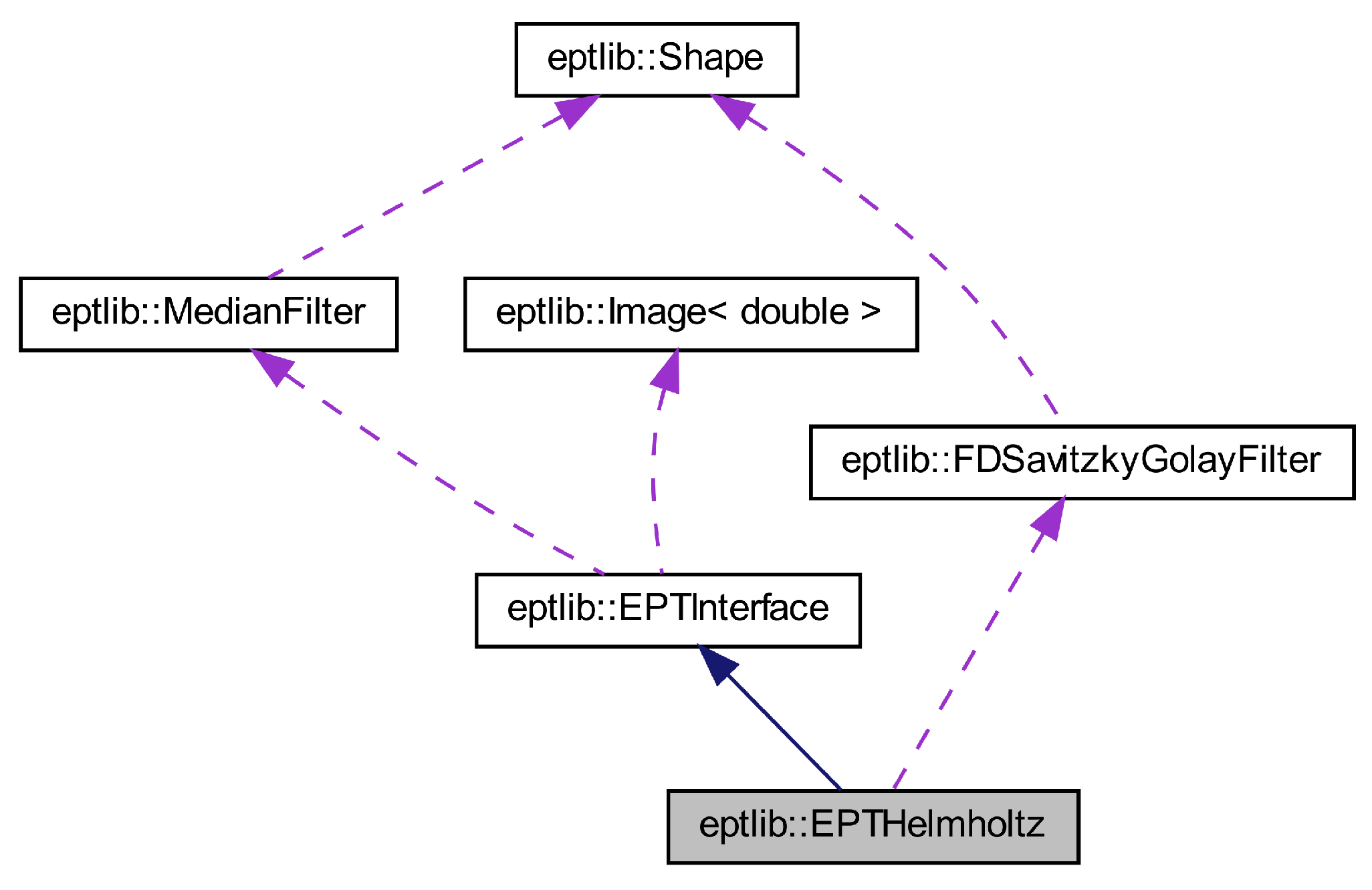
The structure of the library is summarized in Figure 2, where the collaboration diagram of the class implementing Helmholtz-EPT is reported. An identical diagram holds also for the classes implementing convection-reaction-EPT and gradient-EPT. The content of the entire library is protected by the namespace eptlib, that will be omitted when referring to the classes from now on. All the EPT techniques implemented in EPTlib derive from the common abstract class EPTInterface, which provides the elementary methods to handle input and output streams of data and the signature of the method that launches the EPT technique. The abstract class EPTInterface is expected to provide also the post-processing procedures to refine the EPs maps, which can be adopted independently of the used EPT technique. Currently, a median filter is implemented through the class MedianFilter, which reshapes the filter window according to the anatomical geometry deduced from a reference image [9].
The number of input variables can change between different EPT techniques; however, the Tx sensitivity | B 1 + | and the TRx phase φ ± (expressed in radians) are common inputs and, as such, are defined directly in EPTInterface. The number of Tx and receive (Rx) channels can change as well from a technique to another, opening the possibility to exploit multiple Tx sensitivities and TRx phases in input. Similarly, although some techniques could provide additional output variables, the electrical conductivity σ and the relative permittivity ε r are the common output of EPT and so are defined in EPTInterface. Both the input and output common variables are stored as three-dimensional real-valued images through the specialized class template Image<double>, whose import and export as three-dimensional datasets in HDF5 files is handled by library routines.
All the EPT techniques currently implemented in EPTlib are differential techniques that require the computation of the derivatives of the input data. This computation is based on a noise-robust second-order finite difference Savitzky–Golay filter [36] implemented in the class FDSavitzkyGolayFilter. The filter approximates within a moving window the quantity to derive with a second-order polynomial function, which is then derived analytically. In case of a wrapped phase map φ , the derivative is computed observing that
φ = i e i φ e i φ ,
and
2 φ = i 2 e i φ e i φ | e i φ | 2 e i 2 φ ,
in order to avoid the appearance of singularities around the discontinuities of 2 π .
Both the class MedianFilter and the class FDSavitzkyGolayFilter define the filter window by means of an instance of the class Shape, which specializes the features of the Dynamic Bitset of the collection Boost.

2.2. Terminal Application

The terminal application EPTlib_app allows to apply the EPT techniques implemented in the library in a simple way, without the need to know neither the entire library architecture nor the library interface. EPTlib_app is controlled by a TOML configuration file (https://toml.io) that manages the program settings.
Configuration File 1 Common settings for EPTlib_app
1:
title = “Example”
2:
description = “Brief description of the case study”
3:
method = x
4:
[mesh]
5:
    size = [81, 104, 21]
6:
    step = [2 × 10⁻³, 2 × 10⁻³, 2 × 10⁻³]
7:
[input]
8:
    frequency = 64e6
9:
    tx-channels = 2
10:
    rx-channels = 4
11:
    tx-sensitivity = “in.h5:/tx_sens>”
12:
    trx-phase = “in.h5:/trx_phase><”
13:
    wrapped-phase = false
14:
[input.wildcard]
15:
    tx-character = ‘>’
16:
    rx-character = ‘<’
17:
    start-from = 0
18:
    step = 1
19:
[output]
20:
    electric-conductivity = “out.h5:/sigma”
21:
    relative-permittivity = “out.h5:/epsr”
The configuration file has a number of settings common to all the EPT techniques and a parameter section that depends on the selected technique. The common settings, collected in the example Configuration File 1, are described in the following. The first three lines of Configuration File 1 are for basic setups:
  • title and description provide a brief description of the case study.
  • method is an integer value that selects the EPT technique to use according to the following list: 0 for Helmholtz-EPT, 1 for convection-reaction-EPT and 2 for gradient-EPT.
The section mesh describes geometrically the input three-dimensional images:
  • size is the number of voxels of the input data in the three dimensions.
  • step is the length in meters of the voxels in the three dimensions.
The section input defines the input data:
  • frequency is the Larmor frequency in hertz of the input data.
  • tx-channels and rx-channels are the number of Tx and Rx channels in the input data, respectively. They must assume values in certain ranges depending on the adopted EPT technique.
  • tx-sensitivity and trx-phase are the addresses of the Tx sensitivity | B 1 + | and the TRx phase φ ± datasets in suitable HDF5 files. The address is provided as a string in which the HDF5 file address is separated from the internal dataset identifier by a colon. Moreover, in case of multiple Tx channels, the wildcard character ’>’ can be used to distinguish the data from each channel. It will be replaced by an increasing integer number from zero up to the number of Tx channels minus one. Similarly, the wildcard character ’<’ is used for multiple Rx channels. Thus, the string “in.h5:/trx_phase><” denotes the datasets “/trx_phase00”, “/trx_phase10”, “/trx_phase01”, “/trx_phase11”, “/trx_phase02” and so on in the file “in.h5”.
  • wrapped-phase is true if the input TRx phase maps are wrapped. This setting is optional and false by default.
The optional section input.wildcard can be used to change the wildcard characters for the input address definition:
  • tx-character and rx-character are the above-mentioned wildcard character. By default ’>’ and ’<’, respectively.
  • start-from is the integer number from which the wildcard character replacement starts. By default 0.
  • step is the integer step in the wildcard character replacement. By default it is 1.
Lastly, the section output defines the output addresses:
  • electric-conductivity and relative-permittivity are the addresses of the datasets in HDF5 files in which the electric conductivity σ and the relative permittivity ε r estimated by the EPT technique will be stored, respectively. The address is provided as a string in which the HDF5 file address is separated from the internal dataset identifier by a colon. Thus, the string “out.h5:/sigma” denotes the dataset “/sigma” in the file “out.h5”.
For an up-to-date description of the configuration file settings, check the website of EPTlib, https://eptlib.github.io.

3. EPT Techniques

Each EPT technique implemented in EPTlib is accurately described in this section, highlighting the underlying mathematical assumptions and the operative conditions under which it can be applied. The specific settings of the configuration file for EPTlib_app are reported as well.

3.1. Helmholtz-EPT

Assuming a constant magnetic permeability equal to the one of vacuum μ 0 [37], the time-harmonic RF magnetic flux density B 1 generated by the MRI scanner in the biological tissues satisfies
× ε ˜ 1 × B 1 = ω 2 μ 0 B 1 ,
where ω = 2 π f is the angular frequency, being f the Larmor frequency, and  ε ˜ = ε r ε 0 i σ / ω is the complex permittivity, being ε 0 the electric permittivity of vacuum. This equation can be written equivalently as
ε ˜ 1 × × B 1 ε ˜ 1 2 B 1 = ω 2 μ 0 B 1 ,
whose left hand side is deduced from the vector calculus identity × ( × B 1 ) = ( · B 1 ) 2 B 1 and from the Gauss’s law for magnetism · B 1 = 0 . In the regions where the EPs are almost homogeneous, namely ε ˜ 1 0 , the latter coincides with the vector Helmholtz equation.
Since the positively rotating component B 1 + of the RF coil is defined as [38]
B 1 + = B 1 , x + i B 1 , y 2 ,
the Cartesian components of the vector Helmholtz equation can be combined linearly to obtain the Helmholtz equation for B 1 + , which inverted algebraically with respect to ε ˜ leads to the fundamental equation of Helmholtz-EPT [17],
ε ˜ = 2 B 1 + ω 2 μ 0 B 1 + .
Clearly, where the EPs does not satisfy the assumption of homogeneity, like at the tissue boundaries, this equation introduces systematic errors.
By denoting B 1 + = | B 1 + | e i φ + , an explicit equation for each EP can be deduced. Precisely,
ε r = 2 | B 1 + | ω 2 μ 0 ε 0 | B 1 + | + | φ + | 2 ω 2 μ 0 ε 0 ,
and
σ = 2 φ + ω μ 0 + 2 | B 1 + | · φ + ω μ 0 | B 1 + | ,
where the Tx phase φ + is estimated as half of the measurable TRx phase φ ± , when the same RF coil is used both in transmission and in reception with a polarization switch [5].
In the case of | φ + | 2 | 2 | B 1 + | | / | B 1 + | , the relative permittivity can be estimated with the magnitude-based approximation of (7) [18]
ε r 2 | B 1 + | ω 2 μ 0 ε 0 | B 1 + | ,
which underestimates systematically the permittivity. Similarly, when the Tx sensitivity | B 1 + | is enough homogeneous, so that 2 | | B 1 + | · φ + | / | B 1 + | | 2 φ + | , the electric conductivity can be estimated with the phase-based approximation of (8) [18]
σ 2 φ + ω μ 0 .
It is worth noting that the homogeneity of | B 1 + | is often satisfactorily verified by MRI scanners up to 3 T with volume Tx coils [39], since they are designed to achieve it.
It is worth noting that if the Rx sensitivity | B 1 | is almost homogeneous, like in the case of a volume coil used in reception or of an optimized combination of Rx channels [40], the electric conductivity can be estimated by the analogous relation
σ 2 φ ω μ 0 ,
where the complex Rx sensitivity B 1 = | B 1 | e i φ is defined as [38]
B 1 = B 1 , x i B 1 , y 2 .
The combination of (10) and (11) leads to a phase-based approximation that uses directly the measurable TRx phase φ ± = φ + + φ , with no need of estimating φ + ,
σ 2 φ ± 2 ω μ 0 .
Configuration File 2 Helmholtz-EPT specific settings for EPTlib_app
1:
method = 0
2:
[input]
3:
    tx-channels = 1
4:
    rx-channels = 1
5:
[parameter.savitzky-golay]
6:
    size = [2,2,1]
7:
    shape = 0
Helmholtz-EPT is implemented in EPTlib through the class EPTHelmholtz. Since EPTlib applies a Savitzky–Golay filter [36] to estimate the derivatives of the input maps, the terminal application EPTlib_app requires additional settings in the configuration file to determine the filter window. They belong to the optional section parameter.savitzky-golay and are shown in the example Configuration File 2:
  • size is the number of voxels along each semi-axis of the filter window (cf. Figure 3). By default [1,1,1].
  • shape is an integer value that selects the shape of the filter window: 0 for a cross, 1 for an ellipsoid and 2 for a cuboid (cf. Figure 3). By default 0.
Moreover, to apply Helmholtz-EPT it is necessary to select in the configuration file the method 0 and to set tx-channels and rx-channels in the input section equal to 1. If both the input addresses tx-sensitivity and trx-phase are defined in the input section, then the complete Helmholtz-EPT (6) is applied. Otherwise, the magnitude-based approximation (9) or the phase-based approximation (13) is applied, depending on the provided input address.

3.2. Convection-Reaction-EPT

Convection-reaction-EPT overcomes the homogeneity assumption of Helmholtz-EPT by elaborating Equation (4) with no assumptions on the distribution of the EPs. The linearly combination of the x and y components of the vector Equation (4) according to the Tx sensitivity (5) leads to the following equation [19],
γ y i γ x 1 2 B 1 , y x B 1 , x y γ z B 1 + z = γ 2 B 1 + + ω 2 μ 0 B 1 + ,
where the variable γ = ε ˜ 1 has been introduced and the transverse derivatives of the longitudinal component of B 1 (i.e.,  B 1 , z / x and B 1 , z / y ) have been assumed to be negligible. This assumption holds, for instance, around the mid-plane of a birdcage coil, in which case also the longitudinal derivative of B 1 , z would be negligible, and so
· B 1 B 1 , x x + B 1 , y y 0 B 1 + x i B 1 + y i 1 2 B 1 , y x B 1 , x y .
By substituting (15) in (14), the following equation, in which only the measurable component B 1 + of the magnetic flux density appears, is obtained [19],
γ x + i γ y B 1 + x + i B 1 + y γ z B 1 + z = γ 2 B 1 + + ω 2 μ 0 B 1 + .
The conservative form of the latter equation is [41]
· γ β + = ω 2 μ 0 B 1 + ,
being β + = B 1 + i × B 1 + z ^ the convective term.
The latter equation is treated as a complex-valued partial differential equation (PDE) with respect to γ and complemented with Dirichlet boundary conditions, namely the value of γ at the boundary of the computational domain is established a priori. Since, in case of a birdcage coil, Equation (17) holds only around the mid-plane of the coil, where B 1 , z 0 , the determination of the boundary conditions on the top and bottom slices of the region of interest could be tricky. This issue could be avoided by solving the PDE in a single slice with the two-dimensional approximation obtained assuming the longitudinal invariance of the EPs (i.e.,  γ / z 0 ),
x y · γ β x y + + γ 2 B 1 + z 2 = ω 2 μ 0 B 1 + .
Similarly to Helmholtz-EPT, also convection-reaction-EPT admits a phase-based approximation [23]. It can be deduced by observing that if the Tx sensitivity | B 1 + | is almost homogeneous, then Equation (17) is approximated by
· γ β φ + + i γ | φ + | 2 = i ω 2 μ 0 ,
being β φ + = φ + i × φ + z ^ . A similar equation can be deduced for the Rx sensitivity under the assumption of a Rx magnetic flux density whose longitudinal component has negligible derivatives and of an almost homogeneous Rx sensitivity | B 1 | . It reads
· γ β φ + i γ | φ | 2 = i ω 2 μ 0 ,
being β φ = φ + i × φ z ^ . The sum of Equations (19) and (20) leads to
· γ φ ± i · γ × ( φ + φ ) z ^ + i γ | φ + | 2 + | φ | 2 = 2 i ω 2 μ 0 ,
where the TRx phase φ ± = φ + + φ appears. Finally, assuming that σ / ω ε r ε 0 , as it actually is for many biological tissues at 64 M Hz (the Larmor frequency of 1.5 T MRI scanners) [18], it is possible to approximate the unknown as γ i ω / σ . Thus, the imaginary part of (21) reads [23,42]
· ρ φ ± = 2 ω μ 0 ,
where the resistivity ρ = σ 1 has been introduced. Similarly to Equation (18), also (22) can be approximated in two-dimensions assuming that ρ / z 0 .
The PDEs on which convection-reaction-EPT is based are of difficult solution because of the lack of a diffusion term. The introduction of an artificial diffusion term in the equations acts like a viscosity-type regularization of the problem [43] both for the complex-valued Equation (17) and its two-dimensional approximation (18) and for the real-valued phase-based approximation (22). The regularized PDE for the complete convection-reaction-EPT is
λ 2 γ + · γ β + = ω 2 μ 0 B 1 + ,
where λ denotes the artificial diffusion coefficient. An analogous correction is introduced in the other equations.
In EPTlib, the class EPTConvReact manages the convection-reaction-EPT technique. The PDEs are solved numerically according to the finite difference method. The complex-valued PDEs are approximated with second-order centred finite differences, whereas the real-valued PDEs derived by the phase-based approximation are discretized with stable first-order upwind finite differences. In all the cases, the artificial diffusion term is discretized with second-order centred finite differences. The obtained linear system is solved using the biconjugate gradient stabilized method implemented in Eigen 3.
Configuration File 3 Convection-reaction-EPT specific settings for EPTlib_app
1:
method = 1
2:
[input]
3:
    tx-channels = 1
4:
    rx-channels = 1
5:
[parameter.savitzky-golay]
6:
    size = [2,2,1]
7:
    shape = 0
8:
[parameter.dirichlet]
9:
    electric-conductivity = 0.1
10:
    relative-permittivity = 50.0
11:
[parameter]
12:
    volume-tomography = false
13:
    imaging-slice = 3
14:
    artificial-diffusion = true
15:
    artificial-diffusion-coefficient = 0.1
The first- and second-order derivatives of the Tx sensitivity and the TRx phase are estimated by EPTlib applying a Savitzky–Golay filter [36]. Thus, EPTlib_app requires the optional section parameter.savitzky-golay in the configuration file, as described above for Helmholtz-EPT. In addition, it requires the settings reported in the example Configuration File 3 for determining the Dirichlet boundary conditions and selecting the proper PDE. Precisely, the optional section parameter.dirichlet set the Dirichlet boundary conditions as constant values in the entire boundary:
  • electric-conductivity is the electric conductivity in siemens per meter forced at the domain boundary. By default 0. It is worth noting that this condition is used also by the phase-based approximated convection-reaction-EPT (22), in which case the assigned value must be different from zero in order to allow the correct definition of the resistivity ρ .
  • relative-permittivity is the relative permittivity forced at the domain boundary. By default 1.
The optional section parameter selects the two-dimensional approximation (18) and the artificial diffusion regularization (23):
  • volume-tomography is false if the two-dimensional approximation is selected. By default false.
  • imaging-slice is the index of the slice selected for the two-dimensional tomography. This setting is ignored if volume-tomography is true. The mid-plane of the input data is selected by default. If the number of slices is even, then the lower of the two planes in the middle is selected by default.
  • artificial-diffusion is true if the artificial diffusion regularization is adopted. By default false.
  • artificial-diffusion-coefficient is the value of the artificial diffusion coefficient λ . This setting is ignored if artificial-diffusion is false. By default 0.
Moreover, to apply convection-reaction-EPT it is necessary to select in the configuration file the method 1 and to set tx-channels and rx-channels in the input section equal to 1. If both the input addresses tx-sensitivity and trx-phase are defined in the input section, then the complete convection-reaction-EPT (17) is applied. Otherwise, if only trx-phase is defined, the phase-based approximation (22) is applied.

3.3. Gradient-EPT

Gradient-EPT is developed starting from the same equation of convection-reaction-EPT (17), obtained without the assumption of homogeneity of the EPs used by Helmholtz-EPT. However, the computation is significantly different between the two techniques. In particular, gradient-EPT assumes that a parallel transmission (pTx) system with multiple Tx channels is used. In order to distinguish the quantities associated to each Tx channel, they are denoted in the following by the subscript i with reference to the i-th Tx channel.
Being based on Equation (17), gradient-EPT works under the hypothesis that the gradient of the longitudinal component of B 1 , i is negligible, for any channel i. This is verified around the mid-plane of longitudinally symmetric sources, which are usually adopted for volume coils also in pTx systems.
By noting that
1 γ γ = 1 ε ˜ ε ˜ = log ( ε ˜ ) ,
Equation (16) can be conveniently arranged in the equivalent form [20]
B 1 , i + · g + , i g + , g z ω 2 μ 0 ε ˜ B 1 , i + = 2 B 1 , i + ,
where g = log ( ε ˜ ) and g + = g x + i g y have been introduced.
In a pTx system, the positively rotating component B 1 , i + cannot be estimated easily, since the TRx phase does not approximates, in general, the Tx phase. However, assuming that the same Rx coil, or combination of Rx coils, has been used to acquire the signal of each Tx channel, the measured TRx phases φ i ± = φ i + + φ can be combined to estimate the relative Tx phases φ i + , r with respect to a reference Tx phase φ 0 + ,
φ i + , r = φ i ± φ 0 ± = φ i + φ 0 + .
Thus, the positively rotating component of the i-th channel can be written as
B 1 , i + = B 1 , i + , r e i φ 0 + ,
being B 1 , i + , r = | B 1 , i + | e i φ i + , r the measurable part and φ 0 + the unknown reference phase.
Substituting Equation (27) in (25) and cancelling out the common factor e i φ 0 + , the following equation is obtained [20],
i 2 B 1 , i + , r · φ 0 + + B 1 , i + , r · g + , i g + , g z + B 1 , i + , r θ + = 2 B 1 , i + , r ,
where θ + = ω 2 μ 0 ε ˜ + | φ 0 + | 2 i 2 φ 0 + + i φ 0 + · g + , i g + , g z combines the EPs with the other unknown terms. A system of linear equations in the algebraically independent unknowns φ 0 + , g + , g z and θ + is obtained in each voxel by writing Equation (28) for each Tx channel i and solved in the least-squares sense. In order to reduce the presence of numerical artefacts, a linear system is solved using each Tx channel as the reference one; the results are then averaged weighted by the Tx sensitivity magnitude of the corresponding reference channel [20]. An estimate of the EPs can be deduced by combining the unknown terms.
The solution of (28) is the local step of gradient-EPT, which can be followed by a noise-filtering global step, consisting in the solution in the computational domain Ω of the minimization problem [20]
min ε ˜ g + ( ε ˜ ) g + , 0 L 2 ( Ω ) 2 + g z ( ε ˜ ) g z , 0 L 2 ( Ω ) 2 ,
where g + , 0 and g z , 0 denotes the solutions of the local step in each voxel, whilst g + ( ε ˜ ) and g z ( ε ˜ ) are the derivatives of the guess distribution ε ˜ . Considering u = log ( ε ˜ ) as the unknown, problem (29) can be solved by applying the finite element method (FEM) to the associated Euler equation, here reported in weak form for any test distribution v,   
Ω u x + i u y v x i v y + u z v z d V = Ω g + , 0 v x i v y + g z , 0 v z d V .
Since it involves only the derivatives of u, this equation has infinitely many solutions amongst which the correct one must be selected by means of a constraint or a regularization term. In the former case, a number of seed points in which the EPs are constrained to assume certain values is introduced [20]. Numerically, this operation is analogous to setting Dirichlet boundary conditions, although in internal isolated points. In the latter case, a regularization term is added to the minimization problem, which becomes [44]
min ε ˜ g + ( ε ˜ ) g + , 0 L 2 ( Ω ) 2 + g z ( ε ˜ ) g z , 0 L 2 ( Ω ) 2 + λ log ( ε ˜ / ε ˜ 0 ) L 2 ( Ω 0 ) 2 ,
with λ the regularization coefficient, ε ˜ 0 the solution of the local step and Ω 0 Ω the sub-domain where the regularization is applied. The Euler equation associated to the regularized minimization problem (31) for a generic test function v is
+ λ Ω 0 u v d V = + λ Ω 0 log ( ε ˜ 0 ) v d V ,
being the omitted parts equal to (30).
Since the quality of ε ˜ 0 is higher in the homogeneous regions, the sub-domain Ω 0 is defined as the union of the voxels where the EPs are almost homogeneous. The region is identified based on the distribution of the gradient magnitude G = | g + | 2 + | g z | 2 . Precisely, given a tolerance k, Ω 0 is the union of all and only the voxels where G < k max ( G ) . Other definitions of Ω 0 can be found in the literature, like for example definitions based on its extension with respect to the entire computational domain Ω [45].
Because of the large number of small linear systems to be solved in the local step and of the large linear system in the global step, gradient-EPT is computationally the most expensive of the presented techniques. The computational burden can be reduced with a two-dimensional approximation of the equations, which can be obtained under the assumption of the longitudinal invariance of the EPs (i.e.,  g z 0 ) and of the reference phase (i.e.,  φ 0 + / z 0 ). In that case, the equation for the local step (28) becomes
i 2 x y B 1 , i + , r · x y φ 0 + + x y B 1 , i + , r · g + , i g + + B 1 , i + , r θ x y + = 2 B 1 , i + , r ,
with θ x y + = ω 2 μ 0 ε ˜ + | x y φ 0 + | 2 i x y 2 φ 0 + + i x y φ 0 + · ( g + , i g + ) , whereas the global step keeps the same minimization problem (29) without the term relative to g z .
EPTlib implements gradient-EPT in the class EPTGradient, which manages the linear systems using the library Eigen 3 and discretizes the Euler Equations (30) and (32) according to a tri-linear FEM whose elements are the image voxels.
Configuration File 4 Gradient-EPT specific settings for EPTlib_app
1:
method = 2
2:
[input]
3:
    tx-channels = 8
4:
    rx-channels = 1
5:
[parameter.savitzky-golay]
6:
    size = [2,2,1]
7:
    shape = 0
8:
[parameter.seed-point]
9:
    use-seed-point = true
10:
    coordinates = [ [15,20,25], [42,16,20] ]
11:
    electric-conductivity = [0.1, 0.15]
12:
    relative-permittivity = [50.0, 70.0]
13:
[parameter.regularization]
14:
    regularization-coefficient = 1000.0
15:
    gradient-tolerance = 0.01
16:
    output-mask = "out.h5:/mask"
17:
[parameter]
18:
    volume-tomography = false
19:
    imaging-slice = 3
20:
    full-run = true
The example Configuration File 4 collects the additional settings of EPTlib_app specific for gradient-EPT. As already described for Helmholtz-EPT, the optional section parameter.savitzky-golay select the window of the Savitzky–Golay filter [36] adopted for the estimation of the first- and second-order derivatives of the Tx sensitivities and the relative phases in the local step. The optional section parameter.seed-point sets a seed point constraint in the global step (29):
  • use-seed-point is true if the seed point constraint is selected. By default false.
  • coordinates is the list of the integer coordinates of the seed points in the mesh of voxels (index 0 is used for the first voxel). This setting is mandatory if use-seed-point is true, otherwise it is ignored.
  • electric-conductivity is the list of the electric conductivity in siemens per meter forced in each seed point. This setting is mandatory if use-seed-point is true, otherwise it is ignored.
  • relative-permittivity is the list of the relative permittivity forced in each seed point. This setting is mandatory if use-seed-point is true, otherwise it is ignored.
The lists of coordinates, electric-conductivity and relative-permittivity must have as many elements as the number of selected seed points. The optional section parameter.regularization sets the regularization term in the global step (31) if the seed point constraint is not used (this section is ignored if use-seed-point in section parameter.seed-point is true):
  • regularization-coefficient is the value of the regularization coefficient λ . By default 1.
  • gradient-tolerance is the value of the tolerance k for determining the sub-domain Ω 0 . By default 0.
  • output-mask is the address of the dataset in HDF5 file in which the characteristic function of Ω 0 will be stored. The address is provided as a string in which the HDF5 file address is separated from the internal dataset identifier by a colon. Thus, the string “out.h5:/mask” denotes the dataset “/mask” in the file “out.h5”. If this setting is omitted, the data will not be stored.
The optional section parameter selects the two-dimensional approximation (33) and if the execution must end after the local step (28) or proceed with the global-step (29):
  • volume-tomography is false if the two-dimensional approximation is selected. By default false.
  • imaging-slice is the index of the slice selected for the two-dimensional tomography. This setting is ignored if volume-tomography is true. The mid-plane of the input data is selected by default.
  • full-run is false if the execution must stop after the local step. By default true.
Moreover, to apply gradient-EPT it is necessary to select in the configuration file the method 2 and to set rx-channels in the input section equal to 1. Since in the local step (28) there are nine real-valued unknowns and each Tx channel leads to a complex-valued equation, a pTx system with at least five Tx channels is needed by gradient-EPT. Thus, the setting tx-channels in the input section must be at least equal to 5.

3.4. Summary of the Implemented Techniques

Table 1 summarizes the input requirements and the output capabilities of the EPT techniques implemented in EPTlib, distinguishing between possible phase-based and magnitude-based approximations.
Moreover, it is worth recalling the main hypotheses on which the three techniques are based:
  • Helmholtz-EPT assumes that the EPs are locally homogeneous, leading to large systematic errors at the tissue boundaries.
  • The complete versions of both Helmholtz-EPT and convection-reaction-EPT estimate the Tx phase φ + as half of the measurable TRx phase φ ± . This is a reasonable estimation when the same RF coil is used both in transmission and in reception with a polarization switch [5], or when special care is taken in the phase acquisition, like for example adopting a CLEAR reconstruction [46].
  • Both convection-reaction-EPT and gradient-EPT assume that the longitudinal component of B 1 has a negligible gradient. This assumption limits the applicability of these techniques around the mid-plane of longitudinally symmetric sources, which are usually adopted for volume coils.
  • Gradient-EPT requires acquisitions performed with a pTx system with at least five Tx channels. Currently, this kind of equipment is mainly employed in the research of ultra high field scanners.

4. Examples of Application

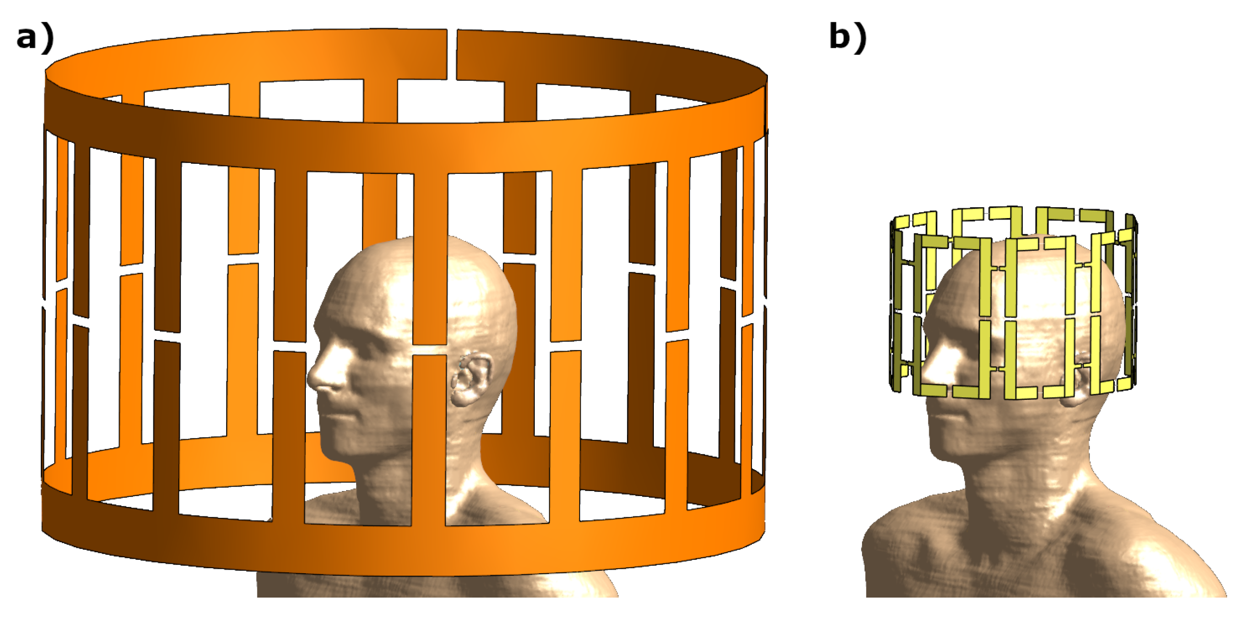
The implemented Helmholtz-EPT and convection-reaction-EPT techniques were applied on virtual data obtained from the simulation of a 1.5 T low-pass 16-leg birdcage body-coil (radius = 36 c m , height = 45 c m ). The body-coil was used both in transmission and in reception with polarization switch. The gradient-EPT technique, instead, was applied on data from the simulation of a 7 T 8-channel head-coil made of eight loops arranged elliptically [47] (height = 16 c m , semi-axes = 11.2 c m and 13.2 c m ). The same head-coil was used in transmission and reception and the raw data acquired by the eight channels were combined according to a circular polarization. Both the coil models were used to perform head imaging of the anatomical human model Duke [48], as illustrated in Figure 4.
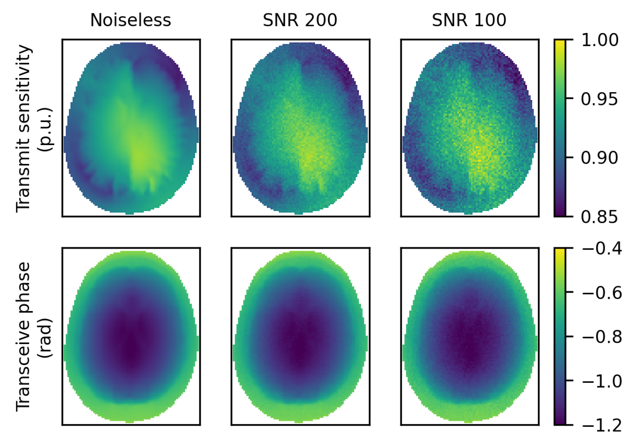
In order to test the EPT techniques in realistic conditions, the simulated sensitivities were sampled on an isotropic Cartesian mesh with sides of 2 m m and were corrupted with additive spatially-uncorrelated Gaussian noise, with a uniform standard deviation and an average signal-to-noise ratio (SNR) of 200 and 100. For the 1.5 T case, the simulated distributions of Tx sensitivity | B 1 + | and TRx phase φ ± are shown in Figure 5, as well as the noisy samples.

4.1. 1.5 T Body-Coil

4.1.1. Helmholtz-EPT

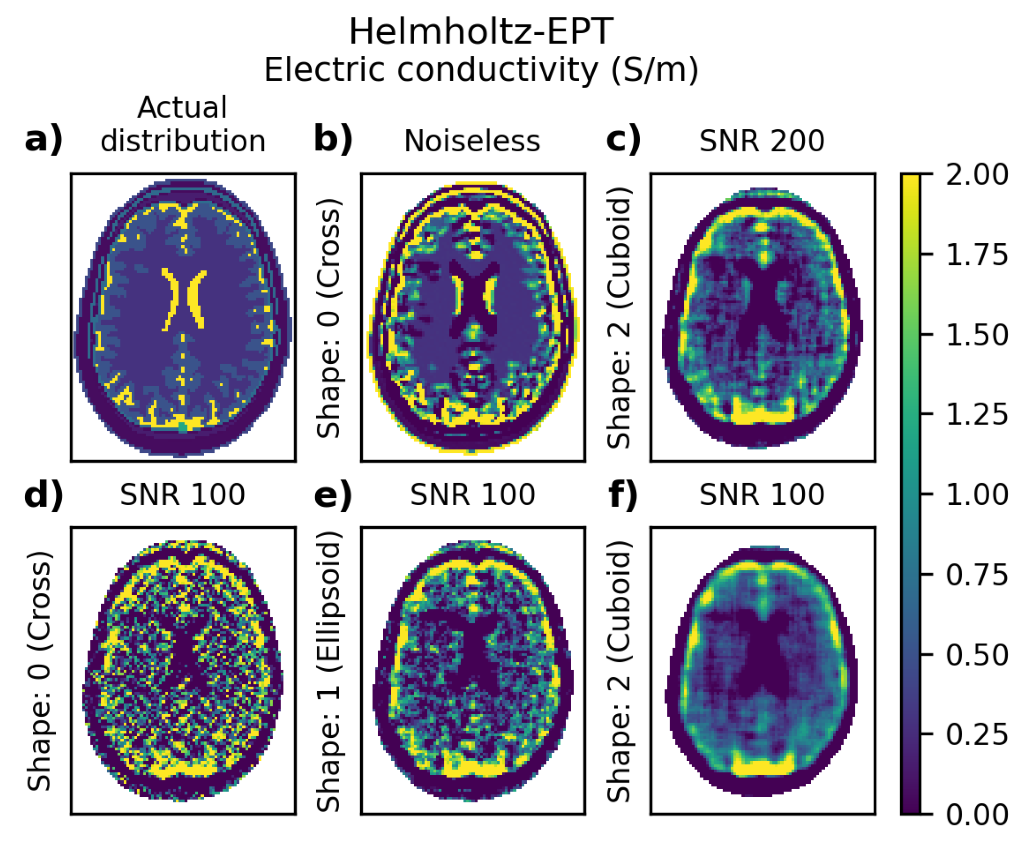
The electric conductivity σ recovered in the mid-plane by applying Helmholtz-EPT on the virtual data generated by the 1.5 T body-coil is reported in Figure 6, where also the actual distribution of σ is shown for comparison. The results were collected for different SNR in the input data and for windows of the Savitzky–Golay filter with various shapes and sizes. The noiseless case (Figure 6b) is elaborated with a minimal filter—the cross of size [1,1,1]—corresponding to the traditional second-order centred finite difference scheme. The large errors introduced at tissue boundaries (including those developed longitudinally and invisible in the two-dimensional map) were due to the assumption of homogeneity of the EPs, on which Helmholtz-EPT was based.
The presence of noise in the case with SNR 200 (Figure 6c) forced us to adopt a wider window for the Savitzky–Golay filter. Precisely, a cuboid of size [2,2,2] was used. This led to a blurred reconstruction, which managed the input noise at the cost of a lower quality. With an amount of noise such that the input SNR was 100, the size of the filter window was further increased to [3,3,3]. In this case, the effect of different window shapes was analyzed by comparing the cross (Figure 6d), the ellipsoid (Figure 6e) and the cuboid (Figure 6f). The cuboid, being the shape that relied on the largest number of voxels, had the strongest damping effect on the input noise, but, at the same time, reduced the effective image resolution by blurring many details.
The considered problem satisfied with large accuracy the assumption of homogeneity of the Tx and the Rx sensitivities. On the one hand, this allowed us to obtain almost identical reconstructions as those reported in Figure 6 if the phase-based approximated Helmholtz-EPT technique was adopted instead of the complete one. On the other hand, the estimation of the relative permittivity ε r was significantly affected by the Laplacian of the Tx sensitivity (7), whose small variations were easily suppressed by the noise. As a consequence, the distributions of ε r recovered by applying Helmholtz-EPT with the adopted filter windows on the noisy input data were extremely noisy and completely unreadable.

4.1.2. Convection-Reaction-EPT

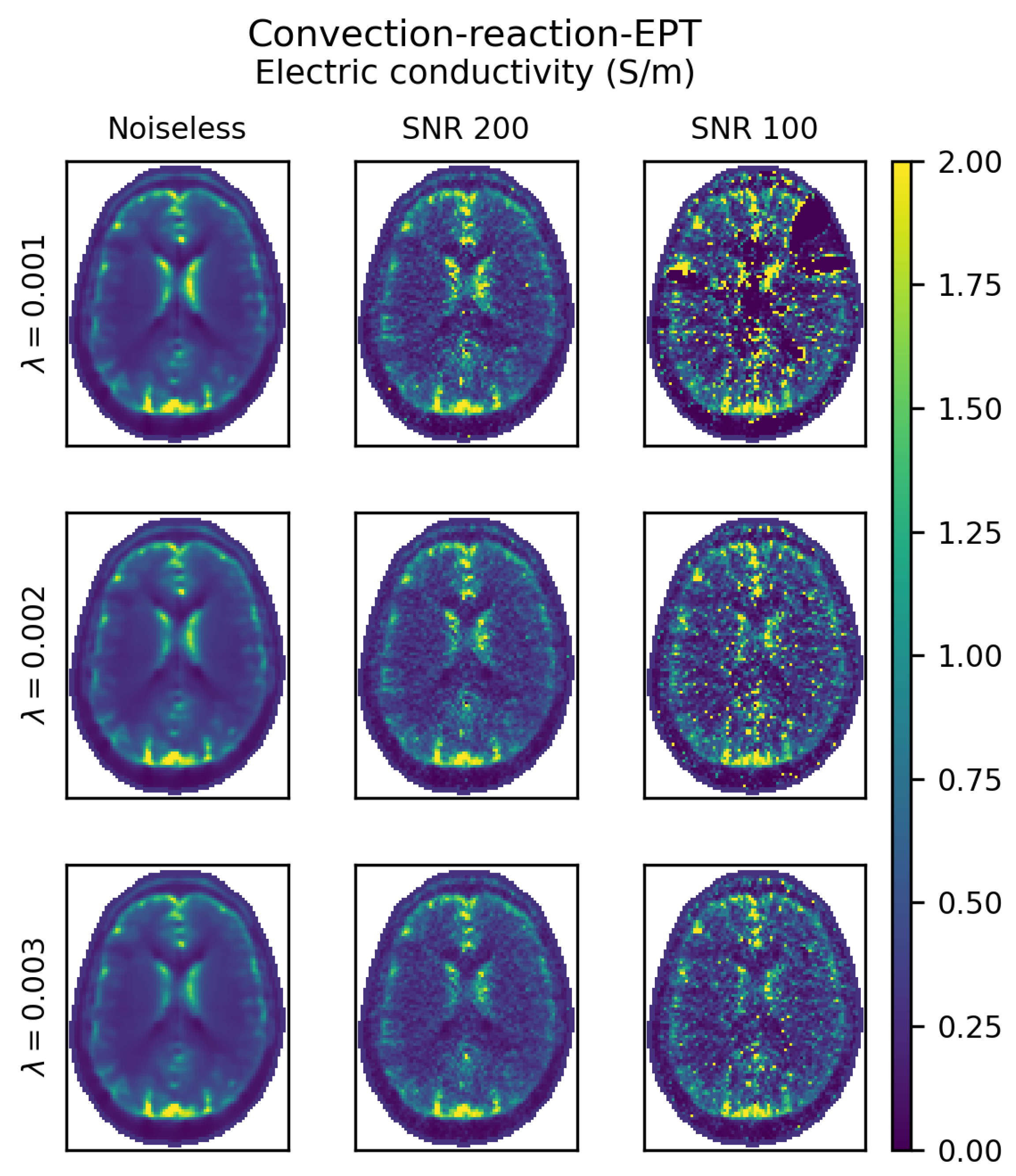
The convection-reaction-EPT technique applied on the complex input data of the simulated 1.5 T body-coil led to extremely ill-conditioned linear systems unless an over-regularization was introduced, making the method unfeasible even in the noiseless case. The results reported in Figure 7 are obtained by the phase-based approximation of convection-reaction-EPT with artificial diffusion regularization applied on a three-dimensional portion of data. Precisely, 21 slices (10 above and 10 below the mid-plane) were considered and found to be enough to reduce the influence of the boundary conditions on the top and bottom slices on the reconstruction in the mid-plane. Figure 7 collects the distribution of σ recovered for different SNR in the input data and different values of the artificial diffusion coefficient λ . All the results were obtained using the minimal Savitzky–Golay filter, namely the cross of size [1,1,1]. The reference distribution of σ was the one reported in Figure 6a.
The reconstructions obtained operating on noiseless data show that a negligible loss of details occurred when the coefficient λ was increased from 0.001 up to 0.003. In particular, a small reduction in the value of the cerebrospinal fluid (CSF) conductivity was observed, with no sensible consequences on the effective image resolution. Moreover, the distributions of σ obtained by convection-reaction-EPT with noiseless input (cf. Figure 7) were significantly improved with respect to the distribution estimated by Helmholtz-EPT (cf. Figure 6b), especially because of the absence of large errors at the tissue boundaries.
When the input data were noisy, the conditioning of the problem at the basis of convection-reaction-EPT worsened, making its resolution more time-consuming and affecting the quality of the result. However, the artificial diffusion term restored the conditioning with a regularization effect that became more relevant when the coefficient λ increased, as can be observed in Figure 7 for the cases with SNR 200 and, more evidently, with SNR 100. It is worth noting that, differently from the increased windows of the Savitzky–Golay filter used for Helmholtz-EPT, the artificial diffusion term managed the noise propagation without affecting significantly the image resolution. The adoption of a large window for the Savitzky–Golay filter in conjunction with the artificial diffusion regularization could help when dealing with very noisy input data.

4.2. 7 T 8-Channel Head-Coil

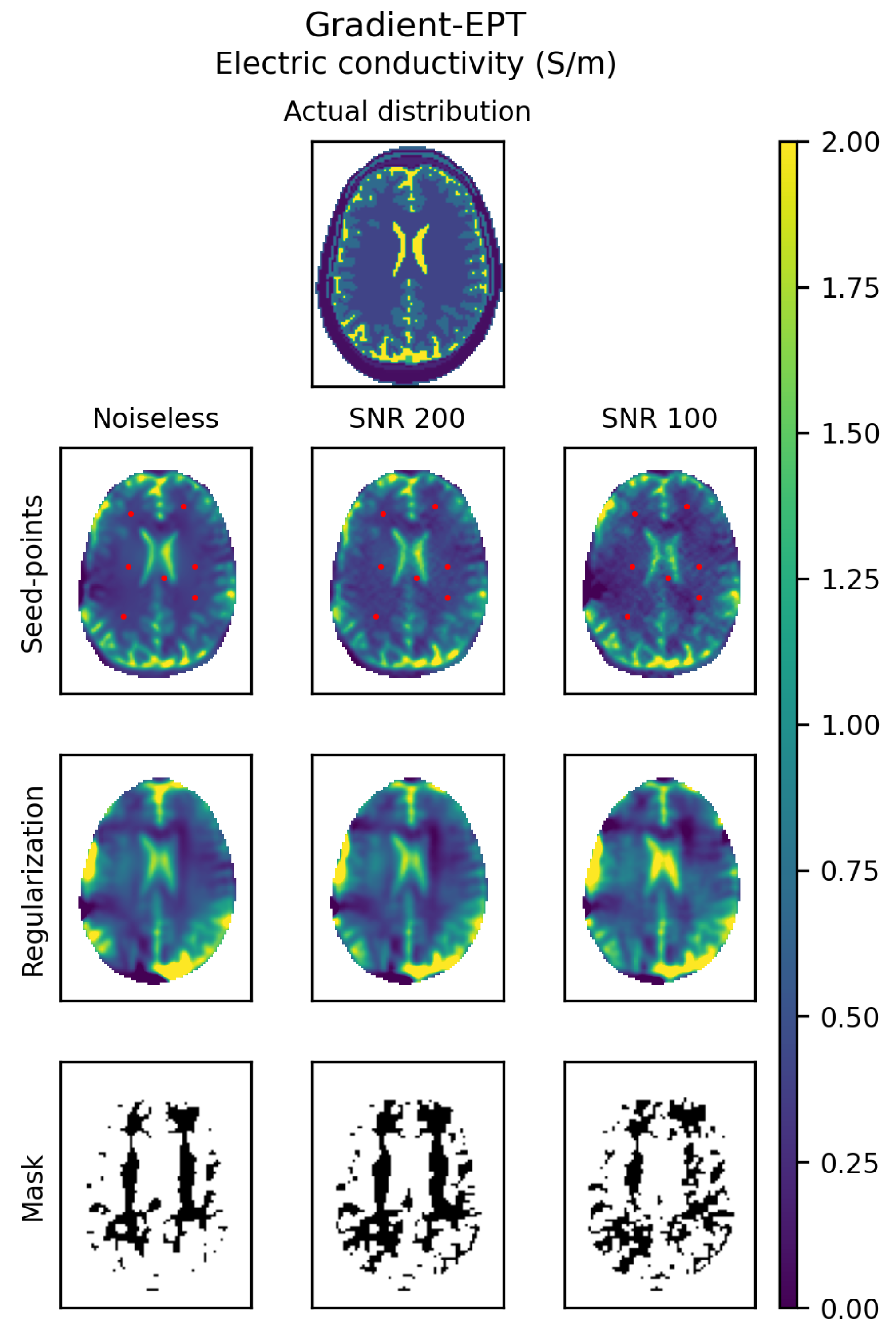
The virtual data generated by simulating the 7 T 8-channel head-coil were used to test the gradient-EPT technique. A three-dimensional portion of data of 11 slices (five above and five below the mid-plane) was used. The obtained distributions of the electric conductivity σ are collected in Figure 8, where the actual distribution of σ at 300 M Hz (the Larmor frequency for 7 T MRI) is reported as well for comparison. The results were collected for different SNR in the input data and were obtained by solving the global step of gradient-EPT with the seed point constraint or with the regularization term. In the former case, a cross of size [2,2,2] was used as window for the Savitzky–Golay filter for any input SNR, whereas in the latter a cuboid of size [2,2,2] was adopted to obtain reasonable outcomes.
Seven seed points distributed in the white matter and located in mid-plane were used for the seed point constrained reconstructions and are pictured as red dots on the recovered maps in Figure 8. The actual EPs of the white matter adopted in the simulations were assigned to the seed points. Their adoption led to an extremely detailed reconstruction of the distribution of σ , even when noisy input data with SNR 100 were used. Regarding the reconstructions obtained with the regularization term, a regularization coefficient λ = 10,000 was used and the regularization mask was determined with a tolerance k = 0.02 for the noiseless input and k = 0.03 for the noisy input. The resulting masks and the recovered distributions of σ , both reported in Figure 8, were very robust with respect to the input noise, although the adoption of a larger window for the Savitzky–Golay filter reduced the effective resolution of the maps with respect to the one obtained with the seed point constraint.
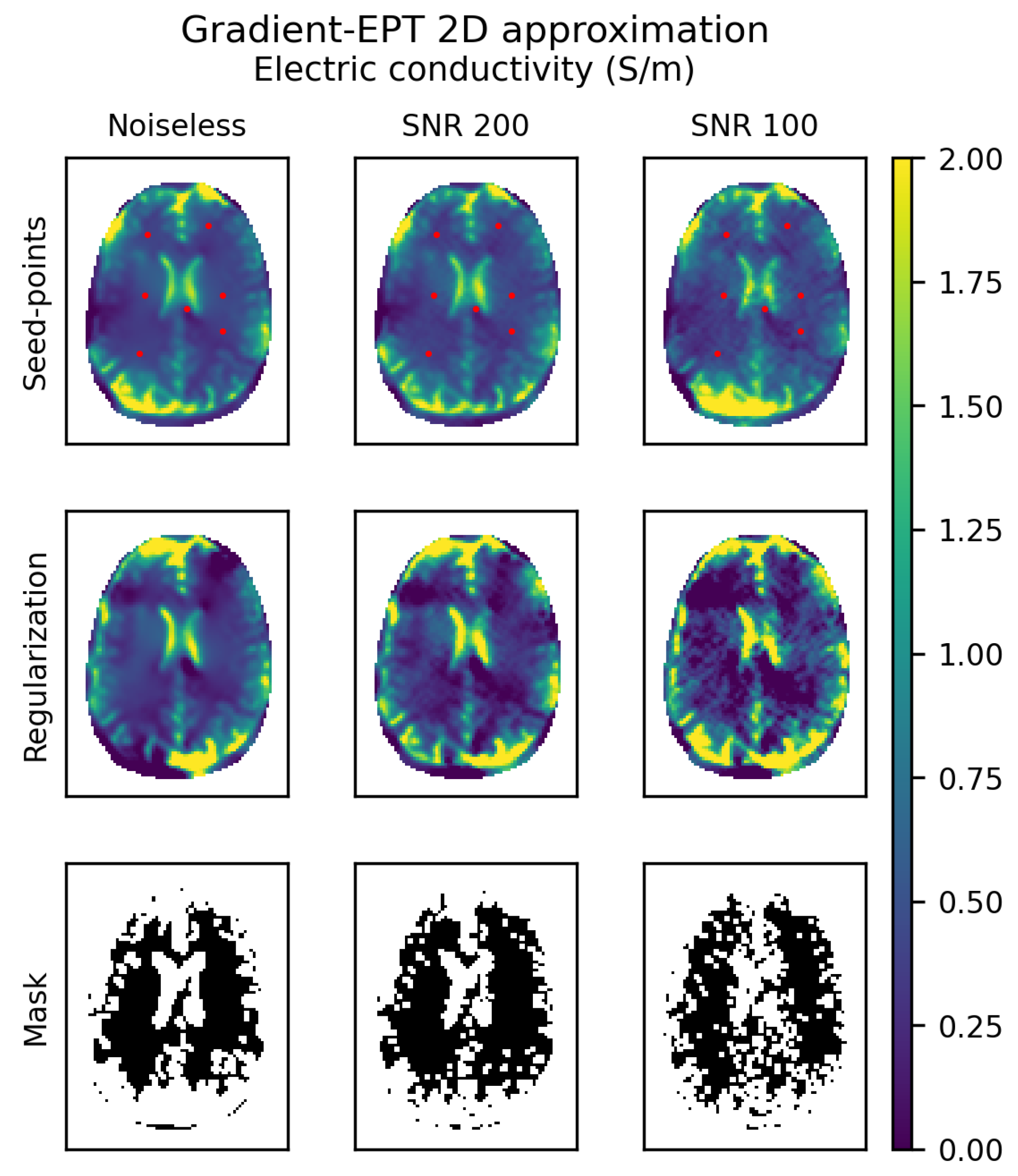
The results obtained by the two-dimensional approximation of gradient-EPT are collected in Figure 9. Besides reducing the computational burden, the two-dimensional approximation simplified the solution of the global step with the regularization term, which in this case was performed, as for the reconstructions obtained with the seed point constraint, using a cross window of size [2,2,2] for the Savitzky–Golay filter. This made the regularized reconstruction more detailed than in the three-dimensional case, although the effect of noise was more relevant. The same seed points used in the three-dimensional case were used also in the two-dimensional approximation with seed point constraint, which led to a reconstruction robust with respect to noise, despite the systematic errors due to the two-dimensional approximation.

5. Conclusions

In this paper, EPTlib, a novel open-source C++ library collecting EPT techniques, has been presented. EPTlib provides a common platform for the implementation and diffusion of EPT techniques at the state of the art, and makes them available and easily accessible to the scientists interested in their applications. The collected techniques are accessible in a ready-to-use form in the terminal application included in EPTlib, which is deeply described in this paper. Updates on the library and its terminal application can be found on the library website https://eptlib.github.io, where examples of usage and datasets are made available as well.
Currently, EPTlib implements three EPT techniques, whose performances when applied on a couple of model problems have been reported to highlight their features and the role of the parameters that can be tuned in the terminal application. Helmholtz-EPT is affected by large errors at the tissue boundaries and, in presence of noise, it requires the adoption of large windows for the Savitzky–Golay filter, reducing the effective resolution of the reconstructed maps. Convection-reaction-EPT, in its phase-based approximated version, provides smoother results than Helmholtz-EPT and reaches higher effective resolutions by handling the noisy input with an artificial diffusion regularization term. Finally, gradient-EPT significantly improves the results of the other techniques by relying on multiple input data. The parameters of each technique should be tuned depending on the noise distribution of the input data. In general, a higher SNR leads to a better effective resolution of the conductivity map, since it allows the adoption of smaller filter windows or lower regularization coefficients. The SNR of the input data could be improved, for instance, by averaging many acquisitions, adopting proper sequences or relying on high field scanners. Despite the differences between the techniques, all the reconstructions are performed in acceptable computational times, since in a laptop PC equipped with an Intel Core i7 at 1.80 G Hz they took at most 30 seconds to solve the model problems.
In the future, EPTlib could become a reference platform for EPT development, helping in its widespread adoption and growing with the implementation of new techniques and the improvement of the ones already implemented.

Funding

The results here presented have been developed in the framework of the EMPIR Project 18HLT05 QUIERO. This project 18HLT05 QUIERO has received funding from the EMPIR programme co-financed by the Participating States and from the European Union’s Horizon 2020 research and innovation programme.

Institutional Review Board Statement

Not applicable.

Informed Consent Statement

Not applicable.

Data Availability Statement

Publicly available open-source software were used in this study. This software can befound here: https://eptlib.github.io.

Acknowledgments

The author wishes to thank the colleagues L. Zilberti, M. Chiampi and O. Bottauscio for the valuable discussions and support provided during the development of the library, and U. Zanovello for the precious set-up of the electromagnetic simulations used to test the implemented techniques. The study reported in this paper is part of the field covered by the European Metrology Network (EMN) for Mathematics and Statistics. Information can be found at https://www.euramet.org/european-metrology-networks/mathmet/.

Conflicts of Interest

The authors declare no conflict of interest. The funders had no role in the design of the study; in the collection, analyses, or interpretation of data; in the writing of the manuscript, or in the decision to publish the results.

References

  1. Ma, D.; Gulani, V.; Seiberlich, N.; Liu, K.; Sunshine, J.L.; Duerk, J.L.; Griswold, M.A. Magnetic resonance fingerprinting. Nature 2013, 495, 187–192. [Google Scholar] [CrossRef] [Green Version]
  2. Venkatesh, S.K.; Yin, M.; Ehman, R.L. Magnetic resonance elastography of liver: Technique, analysis, and clinical applications. J. Magn. Reson. Imaging 2013, 37, 544–555. [Google Scholar] [CrossRef] [Green Version]
  3. Hiscox, L.V.; Johnson, C.L.; Barnhill, E.; McGarry, M.D.J.; Huston, J.; Van Beek, E.J.R.; Starr, J.M.; Roberts, N. Magnetic resonance elastrography (MRE) of the human brain: Technique, findings and clinical applications. Phys. Med. Biol. 2016, 61, R401–R437. [Google Scholar] [CrossRef]
  4. Haacke, E.M.; Petropoulos, L.S.; Nilges, E.W.; Wu, D.H. Extraction of conductivity and permittivity using magnetic resonance imaging. Phys. Med. Biol. 1991, 36, 723–734. [Google Scholar] [CrossRef]
  5. Katscher, U.; Kim, D.-H.; Seo, J.K. Recent progress and future challenges in MR electric properties tomography. Comput. Math. Methods Med. 2013, 2013, 546562. [Google Scholar] [CrossRef] [Green Version]
  6. Liu, J.; Wang, Y.; Katscher, U.; He, B. Electrical properties tomography based on B1 maps in MRI: Principles, applications, and challenges. IEEE Trans. Biomed. Eng. 2017, 64, 2515–2530. [Google Scholar] [CrossRef]
  7. Leijsen, R.; Brink, W.; van den Berg, C.A.T.; Webb, A.; Remis, R. Electrical properties tomography: A methodological review. Diagnostics 2021, 11, 176. [Google Scholar] [CrossRef]
  8. Kim, S.Y.; Shin, J.; Kim, D.H.; Kim, M.J.; Kim, E.-K.; Moon, H.J.; Yoon, J.H. Correlation between conductivity and prognostic factors in invasive breast cancer using magnetic resonance electric properties tomography (MREPT). Eur. Radiol. 2016, 26, 2317–2326. [Google Scholar] [CrossRef]
  9. Tha, K.K.; Katscher, U.; Yamaguchi, S.; Stehning, C.; Teresaka, S.; Fujima, N.; Kudo, K.; Kazumata, K.; Yamamoto, T.; van Cauteren, M.; et al. Noninvasive electrical conductivity measurement by MRI: A test of its validity and the electrical conductivity characteristics of glioma. Eur. Radiol. 2018, 28, 348–355. [Google Scholar] [CrossRef] [PubMed]
  10. Balidemaj, E.; Kok, H.P.; Schooneveldt, G.; van Lier, A.L.H.M.W.; Remis, R.F.; Stalpers, L.J.A.; Westerveld, H.; Nederveen, A.J.; van den Berg, C.A.T.; Crezee, J. Hyperthermia treatment planning for cervical cancer patients based on electrical conductivity tissue properties acquired in vivo with EPT at 3 T MRI. Int. J. Hyperth. 2016, 32, 558–568. [Google Scholar] [CrossRef] [Green Version]
  11. Gavazzi, S.; van Lier, A.L.H.M.W.; Zachiu, C.; Jansen, E.; Lagendijk, J.J.W.; Stalpers, L.J.A.; Crezee, H.; Kok, H.P. Advanced patient-specific hyperthermia treatment planning. Int. J. Hyperth. 2020, 37, 992–1007. [Google Scholar] [CrossRef] [PubMed]
  12. Michel, E.; Hernandez, D.; Lee, S.Y. Electrical conductivity and permittivity maps of brain tissues derived from water content based on T1-weighted acquisition. Magn. Reson. Med. 2017, 77, 1094–1103. [Google Scholar] [CrossRef]
  13. Han, J.; Gao, Y.; Nan, X.; Liu, F.; Xin, S.X. Statistical analysis of the accuracy of water content-based electrical properties tomography. NMR Biomed. 2020, 33, 4273. [Google Scholar] [CrossRef] [PubMed]
  14. Han, J.; Gao, Y.; Nan, X.; Yu, X.; Liu, F.; Xin, S.X. Effect of radiofrequency inhomogeneity on water-content based electrical properties tomography and its correction by flip angle maps. Magn. Reson. Imaging 2021, 78, 25–34. [Google Scholar] [CrossRef]
  15. Yarnykh, V.L. Actual flip-angle imaging in the pulsed steady state: A method for rapid three-dimensional mapping of the transmitted radiofrequency field. Magn. Reson. Med. 2007, 57, 192–200. [Google Scholar] [CrossRef] [PubMed]
  16. Sacolick, L.I.; Wiesinger, F.; Hancu, I.; Vogel, M. B1 mapping by Bloch-Siegert shift. Magn. Reson. Med. 2010, 63, 1315–1322. [Google Scholar] [CrossRef] [Green Version]
  17. Katscher, U.; Voigt, T.; Findeklee, C.; Vernickel, P.; Nehrke, K.; Doessel, O. Determination of electric conductivity and local SAR via B1 mapping. IEEE Trans. Med. Imaging 2009, 28, 1365–1374. [Google Scholar] [CrossRef]
  18. Voigt, T.; Katscher, U.; Doessel, O. Quantitative conductivity and permittivity imaging of the human brain using electric properties tomography. Magn. Reson. Med. 2011, 66, 456–466. [Google Scholar] [CrossRef]
  19. Hafalir, F.S.; Oran, O.F.; Gurler, N.; Ider, Y.Z. Convection-reaction equation based magnetic resonance electrical properties tomography (cr-MREPT). IEEE Trans. Med. Imaging 2014, 33, 777–793. [Google Scholar] [CrossRef] [PubMed] [Green Version]
  20. Liu, J.; Zhang, X.; Schmitter, S.; van de Moortele, P.-F.; He, B. Gradient-based electrical properties tomography (gEPT): A robust method for mapping electrical properties of biological tissues in vivo using magnetic resonance imaging. Magn. Reson. Med. 2015, 74, 634–646. [Google Scholar] [CrossRef] [Green Version]
  21. Lee, S.-K.; Bulumulla, S.; Wiesinger, F.; Sacolick, L.; Sun, W.; Hancu, I. Tissue electrical property mapping from zero echo-time magnetic resonance imaging. IEEE Trans. Med. Imaging 2015, 34, 541–550. [Google Scholar] [CrossRef] [Green Version]
  22. Schmidt, R.; Webb, A. A new approach for electrical properties estimation using a global integral equation and improvements using high permittivity materials. J. Magn. Reson. 2016, 262, 8–14. [Google Scholar] [CrossRef] [PubMed]
  23. Gurler, N.; Ider, Y.Z. Gradient-based electrical conductivity imaging using MR phase. Magn. Reson. Med. 2017, 77, 137–150. [Google Scholar] [CrossRef]
  24. Balidemaj, E.; van den Berg, C.A.T.; Trinks, J.; van Lier, A.L.H.M.W.; Nederveen, A.J.; Stalpers, L.J.A.; Crezee, H.; Remis, R.F. CSI-EPT: A contrast source inversion approach for improved MRI-based electric properties tomography. IEEE Trans. Med. Imaging 2015, 34, 1788–1796. [Google Scholar] [CrossRef]
  25. Ropella, K.M.; Noll, D.C. A regularized, model-based approach to phase-based conductivity mapping using MRI. Magn. Reson. Med. 2017, 78, 2011–2021. [Google Scholar] [CrossRef] [Green Version]
  26. Hong, R.; Li, S.; Zhang, J.; Zhang, Y.; Liu, N.; Yu, Z.; Liu, Q.H. 3-D MRI-based electrical properties tomography using the volume integral equation method. IEEE Trans. Microw. Theory Tech. 2017, 65, 4802–4811. [Google Scholar] [CrossRef]
  27. Rahimov, A.; Litman, A.; Ferrand, G. MRI-based electric properties tomography with a quasi-Newton approach. Inverse Probl. 2017, 33, 105004. [Google Scholar] [CrossRef] [Green Version]
  28. Arduino, A.; Bottauscio, O.; Chiampi, M.; Zilberti, L. Magnetic resonance-based imaging of human electric properties with phaseless contrast source inversion. Inverse Probl. 2018, 34, 084002. [Google Scholar] [CrossRef]
  29. Serrallés, J.E.C.; Giannakopoulos, I.I.; Zhang, B.; Ianniello, C.; Cloos, M.A.; Polimeridis, A.G.; White, J.K.; Sodickson, D.K.; Daniel, L.; Lattanzi, R. Non-invasive estimation of electrical properties from magnetic resonance measurements via global maxwell tomography and match regularization. IEEE Trans. Biomed. Eng. 2020, 67, 3–15. [Google Scholar] [CrossRef]
  30. Mandija, S.; Meliadò, E.F.; Huttinga, N.R.F.; Luijten, P.R.; van den Berg, C.A.T. Opening a new window on MR-based electrical properties tomography with deep learning. Sci. Rep. 2019, 9, 8895. [Google Scholar] [CrossRef] [Green Version]
  31. Gavazzi, S.; den Berg, C.A.T.; Savenije, M.H.F.; Kok, H.P.; Boer, P.; Stalpers, L.J.A.; Lagendijk, J.J.W.; Crezee, H.; Lier, A.L.H.M.W. Deep learning-based reconstruction of in vivo pelvis conductivity with a 3D patch-based convolutional neural network trained on simulated MR data. Magn. Reson. Med. 2020, 84, 2772–2787. [Google Scholar] [CrossRef] [PubMed] [Green Version]
  32. Adler, A.; Lionheart, W.R.B. Uses and abuses of EIDORS: An extensible software base for EIT. Physiol. Meas. 2006, 27, S25–S42. [Google Scholar] [CrossRef] [Green Version]
  33. Borcea, L. Electrical impedance tomography. Inverse Probl. 2002, 18, R99–R136. [Google Scholar] [CrossRef]
  34. Sajib, S.Z.K.; Katoch, N.; Kim, H.J.; Kwon, O.I.; Woo, E.J. Software toolbox for low-frequency conductivity and current density imaging using MRI. IEEE Trans. Biomed. Eng. 2017, 64, 2505–2514. [Google Scholar]
  35. Woo, E.J.; Seo, J.K. Magnetic resonance electrical impedance tomography (MREIT) for high-resolution conductivity imaging. Physiol. Meas. 2008, 29, R1–R26. [Google Scholar] [CrossRef] [PubMed] [Green Version]
  36. Savitzky, A.; Golay, M.J.E. Smoothing and differentiation of data by simplified least squares procedures. Anal. Chem. 1964, 36, 1627–1639. [Google Scholar] [CrossRef]
  37. Collins, C.M.; Yang, B.; Yang, Q.X.; Smith, M.B. Numerical calculations of the static magnetic field in three-dimensional multi-tissue models of the human head. Magn. Reson. Imaging 2002, 20, 413–424. [Google Scholar] [CrossRef]
  38. Hoult, D.I. The principle of reciprocity in signal strength calculations—A mathematical guide. Concepts Magn. Reson. 2000, 12, 173–187. [Google Scholar] [CrossRef]
  39. Van Lier, A.L.H.M.W.; Raaijmakers, A.; Voigt, T.; Lagendijk, J.J.W.; Luijten, P.R.; Katscher, U.; van den Berg, C.A.T. Electrical properties tomography in the human brain at 1.5, 3 and 7T: A comparison study. Magn. Reson. Med. 2014, 71, 354–363. [Google Scholar] [CrossRef]
  40. Lee, J.; Shin, J.; Kim, D.-H. MR-based conductivity imaging using multiple receiver coils. Magn. Reson. Med. 2016, 76, 530–539. [Google Scholar] [CrossRef] [PubMed]
  41. Liu, C.; Jin, J.; Guo, L.; Li, M.; Tesiram, Y.; Chen, H.; Liu, F.; Xin, X.; Crozier, S. MR-based electrical property tomography using a modified finite difference scheme. Phys. Med. Biol. 2018, 63, 145013. [Google Scholar] [CrossRef]
  42. Sun, X.; Lu, L.; Qi, L.; Mei, Y.; Liu, X.; Chen, W. MR-based electrical conductivity imaging using second-order total generalized variation regularization. Appl. Sci. 2020, 10, 7910. [Google Scholar] [CrossRef]
  43. Li, C.; Yu, W.; Huang, S.Y. An MR-based viscosity-type regularization method for electrical properties tomography. Tomography 2017, 3, 50–59. [Google Scholar] [CrossRef] [PubMed]
  44. Liu, J.; Shao, Q.; Wang, Y.; Adriany, G.; Bischof, J.; van de Moortele, P.-F.; He, B. In vivo imaging of electrical properties of an animal tumor model with an 8-channel transceiver array at 7T using electrical properties tomography. Magn. Reson. Med. 2017, 78, 2157–2169. [Google Scholar] [CrossRef]
  45. Wang, Y.; van de Moortele, P.-F.; He, B. CONtrast Conformed Electrical Properties Tomography (CONCEPT) based on multi-channel transmission and alternating direction method of multipliers. IEEE Trans. Med. Imaging 2019, 38, 349–359. [Google Scholar] [CrossRef] [PubMed]
  46. Voigt, T.; Homann, H.; Katscher, U.; Doessel, O. Patient-individual local SAR determination: In vivo measurements and numerical validation. Magn. Reson. Med. 2012, 68, 117–1126. [Google Scholar] [CrossRef] [PubMed]
  47. Seifert, F.; Pfeiffer, H.; Mekle, R.; Waxmann, P.; Ittermann, B. 7T 8-channel pTx head coil with high B1+ efficiency optimized for MRS. Proc. Int. Soc. Mag. Reson. Med. 2016, 24, 3545. [Google Scholar]
  48. Christ, A.; Kainz, W.; Hahn, E.G.; Honegger, K.; Zefferer, M.; Neufeld, E.; Rascher, W.; Janka, R.; Bautz, W.; Chen, J.; et al. The Virtual Family—Development of surface-based anatomical models of two adults and two children for dosimetric simulations. Phys. Med. Biol. 2010, 55, N23–N38. [Google Scholar] [CrossRef]
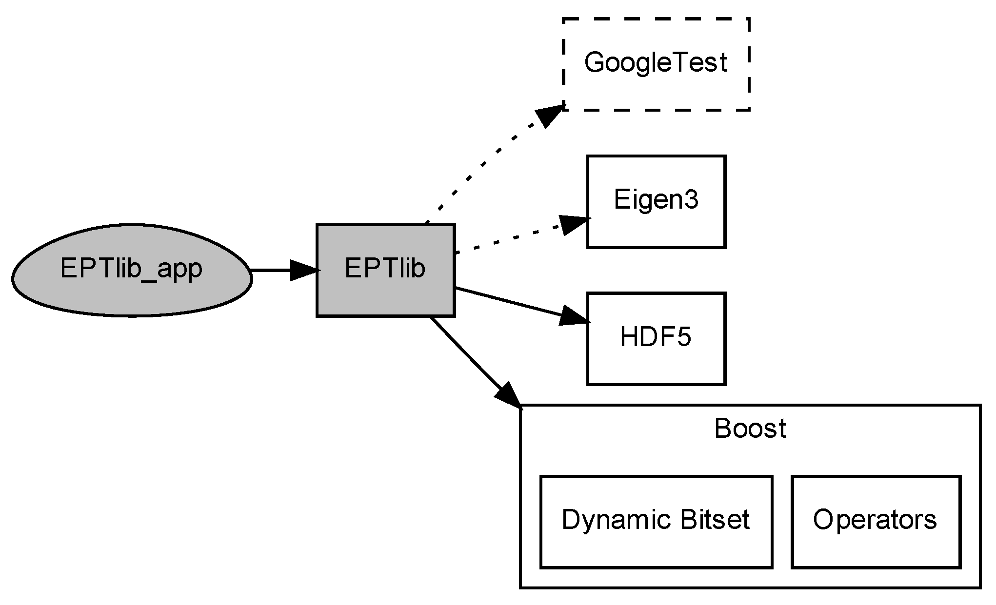
Figure 1. The dependency diagram of the library EPTlib and its terminal application EPTlib_app. The dotted arrow denotes a private dependence, whilst the solid arrow denotes a public one. The dashed box denotes an optional library.
Applsci 11 03237 g001
Figure 2. The collaboration diagram of the class implementing Helmholtz-electric properties tomography (EPT). The dark blue arrow denotes a public inheritance, whilst the purple arrow denotes a collaboration. The classes implementing convection-reaction-EPT and gradient-EPT have an identical collaboration diagram.
Applsci 11 03237 g002
Figure 3. Savitzky–Golay filter windows of different shapes assuming a size equal to [2,2,1].
Applsci 11 03237 g003
Figure 4. RF coils models. (a) 1.5 T low-pass 16-leg birdcage body-coil. (b) 7 T eight-channel head-coil.
Applsci 11 03237 g004
Figure 5. Distributions of the simulated Tx sensitivity | B 1 + | (top) and TRx phase φ ± (bottom) generated by the 1.5 T body-coil in the central section. The effect of additive Gaussian noise is shown as well.
Applsci 11 03237 g005
Figure 6. Electric conductivity distributions recovered by complete Helmholtz-EPT. (a) Actual distribution at 64 M Hz in the considered section. (b) Distribution recovered from noiseless input with a cross window of size [1,1,1] for the Savitzky–Golay filter. (c) Distribution recovered from input with SNR 200 using a cubic window of size [2,2,2] for the Savitzky–Golay filter. (df) Distributions recovered from input with SNR 100 using windows of size [3,3,3] and different shapes (cross, ellipsoid and cuboid, respectively) for the Savitzky–Golay filter.
Applsci 11 03237 g006
Figure 7. Electric conductivity distributions recovered by the phase-based approximation of convection-reaction-EPT with artificial diffusion regularization. All the distributions are recovered using a cross window of size [1,1,1] for the Savitzky–Golay filter. Different artificial diffusion coefficients are used ( λ = 0.001, 0.002 and 0.003) on input data with different amounts of noise (noiseless, signal-to-noise ratio—SNR = 200 and SNR = 100). To be compared with the actual distribution at 64 M Hz reported in Figure 6a.
Applsci 11 03237 g007
Figure 8. Electric conductivity distributions recovered by gradient-EPT and actual distribution at 300 M Hz . The distributions recovered with the seed point constraint use a cross window of size [2,2,2] for the Savitzky–Golay filter. The selected seed points are marked by red dots. The distributions recovered with regularization use a cuboid window of size [2,2,2] for the Savitzky–Golay filter and a regularization coefficient λ = 10,000. The masks adopted for regularization are obtained with a tolerance k = 0.02 in the noiseless case and k = 0.03 in the noisy cases. The resulting masks are reported. Results obtained with different amount of noise (noiseless, SNR = 200 and SNR = 100) are collected.
Applsci 11 03237 g008
Figure 9. Electric conductivity distributions recovered by the two-dimensional approximation of gradient-EPT, to be compared with the actual distribution at 300 M Hz reported in Figure 8. All the distributions are recovered using a cross window of size [2,2,2] for the Savitzky–Golay filter. The seed points selected for the constraint are marked by red dots. The distributions recovered with regularization used a regularization coefficient λ = 1000 . The masks adopted for regularization were obtained with a tolerance k = 0.02 in the noiseless case, k = 0.03 with SNR 200 and k = 0.05 with SNR 100. The resulting masks are reported. Results obtained with different amount of noise (noiseless, SNR = 200 and SNR = 100) were collected.
Applsci 11 03237 g009
Table 1. Summary of the input requirements and output capabilities of the EPT techniques implemented in EPTlib.
InputOutput
Tx Chan.Rx Chan.Tx Sens.TRx Phase σ ε r
Helmholtz-EPT:
Complete1 a
Phase-based1 a
Magnitude-based1 a
Convection-reaction-EPT:
Complete1 a
Phase-based1 a
Gradient-EPT:
Complete≥5 a
a In case of multiple Rx channels, they can be combined before passing the data to EPTlib_app.
Publisher’s Note: MDPI stays neutral with regard to jurisdictional claims in published maps and institutional affiliations.