Article

A Partially Interpretable Adaptive Softmax Regression for Credit Scoring

by
Lkhagvadorj Munkhdalai
1,
Keun Ho Ryu
2,3,*,
Oyun-Erdene Namsrai
4,* and
Nipon Theera-Umpon
3,5
1
Database/Bioinformatics Laboratory, College of Electrical and Computer Engineering, Chungbuk National University, Cheongju 28644, Korea
2
Faculty of Information Technology, Ton Duc Thang University, Ho Chi Minh 700000, Vietnam
3
Biomedical Engineering Institute, Chiang Mai University, Chiang Mai 50200, Thailand
4
Department of Information and Computer Sciences, National University of Mongolia, Sukhbaatar District, Building#3 Room#212, Ulaanbaatar 14201, Mongolia
5
Department of Electrical Engineering, Faculty of Engineering, Chiang Mai University, Chiang Mai 50200, Thailand
*
Authors to whom correspondence should be addressed.
Appl. Sci. 2021, 11(7), 3227; https://doi.org/10.3390/app11073227
Submission received: 8 March 2021 / Revised: 25 March 2021 / Accepted: 31 March 2021 / Published: 3 April 2021
(This article belongs to the Special Issue Data Technology Applications in Life, Diseases, and Health)

Abstract

:
Credit scoring is a process of determining whether a borrower is successful or unsuccessful in repaying a loan using borrowers’ qualitative and quantitative characteristics. In recent years, machine learning algorithms have become widely studied in the development of credit scoring models. Although efficiently classifying good and bad borrowers is a core objective of the credit scoring model, there is still a need for the model that can explain the relationship between input and output. In this work, we propose a novel partially interpretable adaptive softmax (PIA-Soft) regression model to achieve both state-of-the-art predictive performance and marginally interpretation between input and output. We augment softmax regression by neural networks to make it adaptive for each borrower. Our PIA-Soft model consists of two main components: linear (softmax regression) and non-linear (neural network). The linear part explains the fundamental relationship between input and output variables. The non-linear part serves to improve the prediction performance by identifying the non-linear relationship between features for each borrower. The experimental result on public benchmark datasets shows that our proposed model not only outperformed the machine learning baselines but also showed the explanations that logically related to the real-world.

1. Introduction

Credit scoring is a numerical expression of a borrower’s creditworthiness that is estimated by credit experts based on applicant information using statistical analysis or machine learning models. In recent years, many machine learning models have been developed to achieve higher predictive accuracy for classifying borrowers as bad or good [1,2]. However, the inability to explain these machine learning models is one of the notable disadvantages. Financial institutions usually want to understand decision-making process of machine learning models to trust them [3,4]. Therefore, there is still a need for credit scoring model that can improve the predictive performance and its interpretation [5,6]. Without model explanations, machine learning algorithms cannot be adopted by financial institutions and would likely not be accepted by consumers [7].
From a machine learning perspective, the credit scoring problem is considered an imbalanced binary classification task because the number of bad borrowers tends to be much lower than the number of good borrowers in real-life [8,9,10,11]. As bad borrowers occur infrequently, standard machine learning models usually misclassify the bad borrowers compared to the good borrowers.
In this work, we aim to overcome these tricky issues by proposing a novel partially interpretable adaptive softmax regression (PIA-Soft) model augmented by deep neural networks to make its estimated probabilities adaptive for each class (see Figure 1). We first compute a linear transformation of input variables based on the softmax regression to obtain logits for each borrower. Secondly, we also perform a neural network (non-linear part) to augment logit of each class to make them adaptive for dealing with an imbalance problem. Finally, the summed linear and non-linear (output of neural network) transformations are fed into the softmax function to the probability of each class. The linear part partially explains the fundamental relationship between input and output variables, and the nonlinear part serves to improve the prediction performance by identifying the non-linear relationship between features for each borrower. The PIA-Soft architecture we propose is similar to the residual neural network model (ResNet), with the linear transformation acting as a residual block [12]. However, the advantage over ResNet architecture is that the PIA-Soft model can be partially explainable.
To show achievement of the proposed model, we compare our model to high-performance machine learning benchmarks such as Logistic Regression, Random Forest, AdaBoost, XGBoost, Neural Network, LightGBM, Catboost, and TabNet [13,14,15,16,17,18,19,20]. We apply our proposed model to over four benchmark real-world credit scoring datasets. The model performance on the test set is evaluated against three theoretical measures, an area under the curve (AUC), f-score, g-mean, and accuracy [21]. Our proposed model significantly outperformed machine learning models in terms of predictive performance. In order to evaluate the interpretation of PIA-Soft model, we compare our result to logistic regression because this model is the most popular white-boxing approach that is commonly used on credit scoring application. Here are some properties of logistic regression that make it a major benchmark—good predictive accuracy, high-level interpretability, and the modeling process is faster and easier [22]. Therefore, we can utilize it to verify the trustworthiness of our proposed model by comparing its unbiased estimated coefficients for input variables.
In the end, the main contributions of this paper are included as follows:
  • To achieve high predictive accuracy, usually, model complexity is increased. Therefore, machine learning models often make a deal with the predictive performance and interpretable predictions. We propose a model with both high predictive ability and partially explainable.
  • In order to handle class imbalance problem without sampling techniques, our proposed model is designed.
  • We extensively evaluate PIA-Soft model on four benchmark credit scoring datasets. The experimental results show that PIA-Soft achieves state-of-the-art performance in increasing the predictive accuracy, against machine learning baselines.
  • It has proven that our proposed model could explore the partial relationship between input and target variables according to experiments on real-world datasets.
This work is organized as follows: Section 2 presents previous research on the topics related to machine learning models for credit scoring. We introduce the concept of the methods explored in this paper and critically evaluate tools and methodologies available to the date. Section 3 describes our proposed model in more detail. Section 4 indicates the benchmark datasets and comparison of experimental results. This section presents the predictive performance and comparison of PIA-Soft with logistic regression for model interpretability. Finally, Section 5 concludes and discusses the general findings from this work.

2. Related Work

During the past decades, machine learning models have been widely used in many real-life applications such as speech recognition, object detection, healthcare, genomics, and many other domains [23]. In credit scoring application, the researchers have been applied many types of machine learning algorithms such as discriminant analysis, logistic regression, linear and quadratic programming, decision trees, and neural networks [1,2,3,4,5,6,7,8,9,10]. We review such machine learning classification algorithms that are proposed for credit scoring. We also summarize the strengths and weaknesses of current credit scoring models, which used machine learning models, and drew some practical issues that serve as a foundation in this work.
Louzada, Ara and Fernandes [24] studied a systemic literature review relating theory and application of binary classification techniques for credit scoring. They reviewed 187 papers in this field and defined the percent of main classification algorithms such as logistic regression (10.9%), neural network (17.6%), hybrid models (16.8%), ensemble models (16.0%), support vector machine (14.3%), decision trees (6.7%), and others (24.4%).

2.1. Benchmark Classification Algorithms

Advanced machine learning techniques, however, are quickly gaining applications throughout the financial services industry, transforming the treatment of large and complex datasets. Still there is a massive gap between their ability to build robust predictive models and their ability to understand and manage those models [25,26,27,28,29,30]. Logistic regression is a powerful technique that commonly used in practice because it satisfies the huge gap as a mentioned above. The only major disadvantage of logistic regression is that its predictive ability seems to be weaker than other state-of-the-art machine learning models.
Another benchmark machine learning model in this field is neural networks. Firstly, West [31] applied five different neural network architectures for the credit scoring problem. They showed the mixture-of-experts and radial basis function-based neural network models must consider for credit scoring models. Since then, many neural network models have been suggested to tackle the credit scoring problem such as the probabilistic neural network [32], partial logistic neural network model [33], artificial metaplasticity neural network [34], and hybrid neural networks [28]. The neural network models achieved the highest average correct classification rate compared to other traditional techniques, such as discriminant analysis and logistic regression [35]. Although the neural network models achieve a higher predictive accuracy of the borrowers’ creditworthiness, their decision-making process is rarely understood because of the models’ black-box nature.
Recently, many ensemble and hybrid techniques with high predictive performance have been proposed for credit scoring application [36,37,38,39,40]. The ensemble procedure applies to methods of combining classifiers, whereby multiple techniques are employed to solve the same problem in order to boost credit scoring performance. An earlier work is that Maher and Abbod [36], who introduced a new classifier combination technique based on the consensus approach of different machine learning algorithms during the ensemble modeling phase. Their proposed technique significantly improved prediction performance against baseline classifiers. Another work proposed an ensemble classification approach based on a supervised clustering algorithm [37]. They applied supervised clustering to partition the data samples of each class into several of clusters and construct a specific base classifier for each subset. After that, the outputs of these base classifiers are combined by weighted voting. The results showed that compared to other ensemble methods, this approach is able to generate base classifiers with higher diversity and local accuracy and improve the accuracy of credit scoring. In addition, using a combination of deep learning and ensemble techniques improved the predictive performance of credit scoring [38]. Many researchers have also proposed an effective imbalanced learning approach based on a multi-stage ensemble framework [39,40]. These frameworks usually aim to balance the data in the first stage, and the ensemble models learn to obtain a superior predicted result adapting to different imbalance ratios.
For our proposed model, a neural network produces additional logit for each class to make them adaptive to deal with an imbalance problem during the training phase.

2.2. Explainable Credit Scoring Model

Another line of research is related to an explainable credit scoring model, which is to understand how a borrower’s scoring is calculated. More recently, the state-of-the-art machine learning models have achieved human-level performance in many fields, making it very popular [3]. Although these models have reached high predictive performance, the inability to explain them decreases humans’ trust. Therefore, explainable artificial intelligence (XAI) has become very popular in credit scoring problem. XAI aims to make the model understandable and trustworthy.
Many researchers have made great efforts to improve the model understandability and increase humans’ trust. Ribeiro et al. [41] proposed the LIME technique, short for Local Interpretable Model-agnostic Explanations, in an attempt to explain any decision process performed by a black-box model. LIME explains any classifier’s predictions in an interpretable and faithful manner, by learning an interpretable model locally around the prediction. The disadvantage of LIME, however, is that because LIME is based on surrogate models, it can critically reduce the quality of explanations provided. Another popular method for explaining black-box models is SHapley Additive eXplanations (SHAP) [42]; SHAP are Shapley values representing the feature importance measure for a local prediction and are calculated by combining insights from six local feature attribution methods. The Shapley value can be misinterpreted because the Shapley value of a variable value is not the difference of the predicted value after removing the variable from the dataset. Many researchers have applied these two methods with state-of-the-art machine learning algorithms for making explainable models in credit scoring application [4,7,43,44,45].
In addition, Fair Isaac Corporation (FICO) announced the Explainable Machine Learning Challenge to aim generating new research in the credit scoring domain of model explainability [46]. The winners proposed Boolean Rules via Column Generation (BRCG), a new interpretable model for binary classification where Boolean rules in disjunctive normal form (DNF) or conjunctive normal form (CNF) are learned [47]. Although this model has achieved both good classification accuracy and explainability, the authors mentioned that limitations include performance variability and the affected solution quality for large datasets.
However, with regards to credit scoring application, we first need to understand what kind of model the explainable model is [48]. Although the requirements of explainable model depends directly on its user, the explainable credit scoring model should answer the following questions: (1) loan officers often want to understand how the borrower’s indicators, such as age, income, etc., affect borrower’s credit score; (2) rejected loan applicants want to know why they could not satisfy the lender’s requirements; (3) regulators want to understand the reasoning behind the general logic used by the model when making its predictions. In order to answer these two questions, it is important to measure the impact of each variable on the borrower’s default probability. By determining the impact of variables on a borrower’s default probability, we can explain the behavior of models by capturing the relationship between input variables and their direction. To provide these explanations marginally, we attempt to obtain a partial explanation of the model without depreciating its predictive performance.

3. Methodology

3.1. Softmax Regression

Softmax regression is a generalization of logistic regression to handle multiple classes [49]. In this work, in order to produce a linear logit for each class, we use softmax regression for binary classification tasks. We assume that the classes were binary: y ( i ) { 0 ,   1 } . Our training set consists of n . labeled observations {( x ( 1 ) ,   y ( 1 ) ), … ( x ( n ) ,   y ( n ) )}, where the input variables are x ( 1 )   m . Our hypothesis took the form:
h θ ( x ) = [ P ( y = 0 | x ; θ ) P ( y = 1 | x ; θ ) ] = 1 j = 0 1 exp ( θ ( j ) Τ x ) [ exp ( θ ( 0 ) Τ x ) exp ( θ ( 1 ) Τ x ) ]
where θ ( 1 ) ,   θ ( 2 ) m are the weight parameter of softmax regression. From here, our cost function will be
( θ ) = [ i = 1 n ( 1 y ( i ) ) log ( 1 h θ ( x ( i ) ) ) + y ( i ) log ( h θ ( x ( i ) ) ) ] = [ i = 1 n j = 0 2 1 { y ( i ) = j } log P ( y ( i ) = j | x ( i ) ; θ ) ]
In our proposed model, we will make a linear transformation or logit { θ ( j ) Τ x } as adaptable using neural networks.

3.2. Neural Networks

We apply a multilayer perceptron (MLP) as an adaptation model to update the logit of softmax regression. MLP is the most commonly used type of feed-forward artificial neural network that has been developed similar to human brain function; the basic concept of a single perceptron was introduced by Rosenblatt [17]. This network consists of three layers with completely different roles called input, hidden, and output layers. Each layer contains weight parameters that link a given number of neurons with the activation function and neurons in neighbor layers. The form of MLP with a single hidden layer can be represented as follows:
f ω , b ( x ) = G ( ω ( 2 ) ( H ( ω ( 1 ) x + b ( 1 ) ) ) + b ( 2 ) )
where ω ( 1 ) ,   ω ( 2 ) are weight parameters, b ( 1 ) ,   b ( 2 ) are bias parameters and G and H are activation functions.
MLP achieves the optimal weight and bias parameters by optimizing objective function using a backpropagation algorithm to construct a model as
( ω , b ) = [ i = 1 n ( 1 y ( i ) ) log ( 1 f ω , b ( x ( i ) ) ) + y ( i ) log ( f ω , b ( x ( i ) ) ) ] = [ i = 1 n j = 0 2 1 { y ( i ) = j } log P ( y ( i ) = j | x ( i ) ; ω ; b ) ]

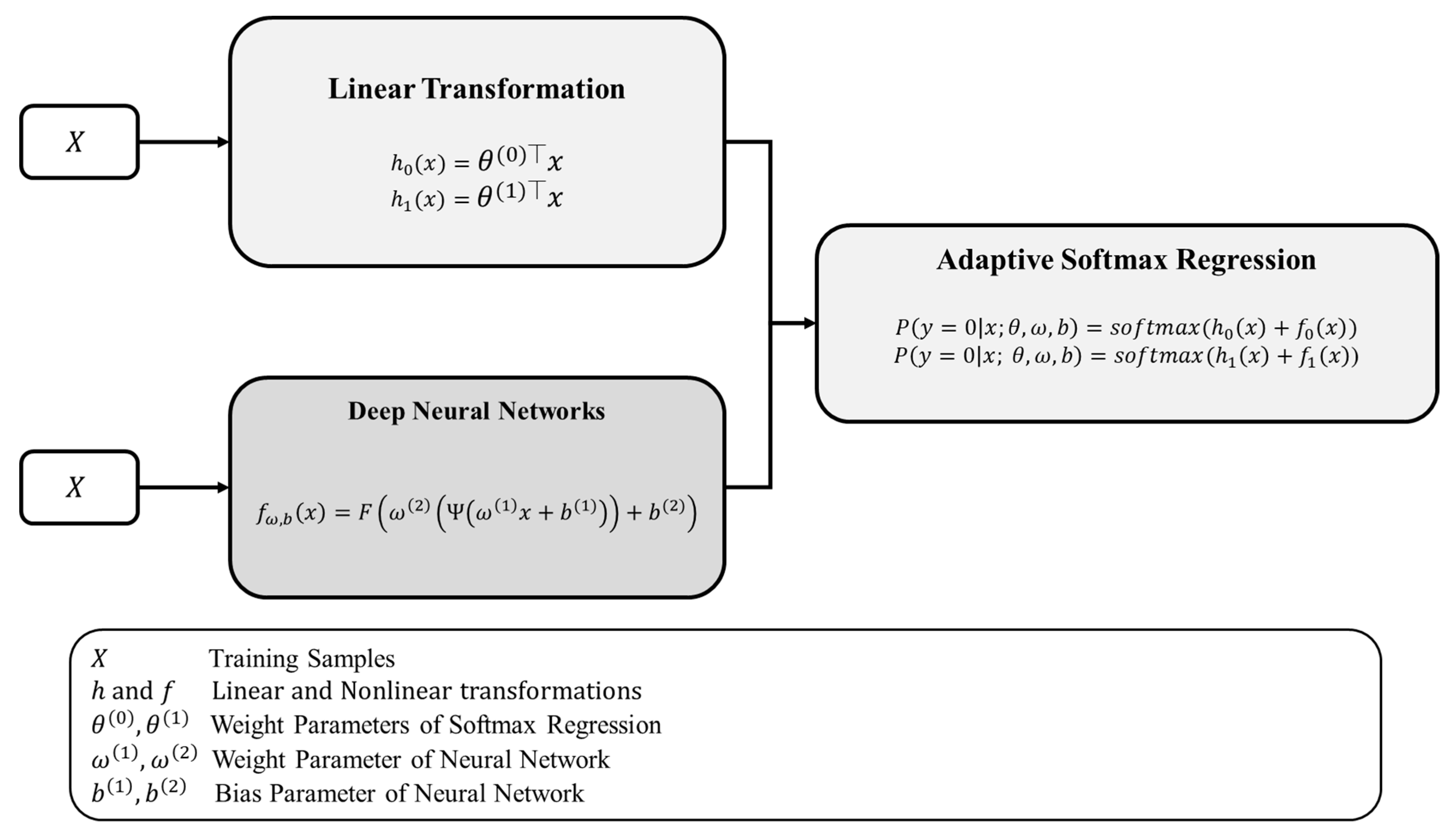
3.3. A Partially Interpretable Adaptive Softmax Regression (PIA-Soft)

The overall architecture of adaptive softmax regression for credit scoring is as shown in Figure 2. We first compute a linear transformation of input variables and weight parameters of softmax regression to obtain a logit for each observation. We then perform a neural network to augment the logit to adapt them for each observation to deal with an imbalance problem. Finally, summed linear transformation and output of the deep neural network is then fed into the softmax function to estimate each class’s probability.
y = s o f t max ( h θ ( x ) + f ω , b ( x ) )
where h θ . define linear transformation (softmax regression) and f ω ,   b defines non-linear transformation (neural network).
In addition, we jointly optimize softmax regression and neural networks in the end-to-end framework. Our loss function for adaptive softmax regression is constructed as follows:
( θ , ω , b ) = [ i = 1 n ( 1 y ( i ) ) log ( 1 ( f ω , b ( x ( i ) ) + h θ ( x ( i ) ) ) ) + y ( i ) log ( f ω , b ( x ( i ) ) + h θ ( x ( i ) ) ) ] = [ i = 1 n j = 0 2 1 { y ( i ) = j } log P ( y ( i ) = j | x ( i ) ; θ ; ω ; b ) ]

4. Experimental Results

4.1. Dataset

Our adaptive softmax regression models is compared with benchmark machine learning algorithms in terms of four real-world credit datasets. Three datasets from UCI repository [50], namely, Australian and Taiwan, and other one dataset from FICO’s explanation machine learning challenge [47], namely, FICO. A summary of all the datasets is presented in Table 1.

4.2. Machine Learning Baselines and Hyperparameter Setting

For the PIA-Soft model, we used the same neural network architecture for all datasets. The neural network contains two hidden layers with 32 neurons. For hyper-parameters: learning rate, batch size, and epoch number must be pre-defined to train a model. We set the learning rate to 0.001, epoch number for training to 3000 and use a mini-batch with 32 instances at each iteration. An Early Stopping algorithm is used for finding the optimal epoch number based on given other hyper-parameters.
For benchmark models, Logistic regression, which have been the most widely used method for binary classification task [13].
Random Forest classification [14], which is ensemble learning method defined as an aggregation of a multiple decision tree classifiers.
AdaBoost classification [15], which is boosting algorithm that focuses on classification problems and aims to combine a set of weak classifiers into a strong one. We use a base estimator as a Decision tree classification.
XGBoost classification [16], which is a boosting ensemble algorithm, optimizes the objective of function, size of the tree and the magnitude of the weights are controlled by standard regularization parameters. This method uses Classification and Regression Trees (CART).
LightGBM [17] and CatBoost [18] are fast, distributed, high-performance gradient boosting models based on decision tree algorithm, used for classification and many other machine learning tasks.
TabNet [19] model is similar to simpler tree-based models while benefiting from high performance, almost identical to deep neural networks.
We also use exactly identical architecture to the neural network benchmark with adaptive softmax regression. The hyper-parameters of these baseline classifiers are optimized by random search with 10 cross-validation methods over parameter settings, as shown in Table 2.
In addition, we apply the most widely used re-sampling techniques with machine learning baselines on the public datasets. The resampling techniques include:
SMOTE: Synthetic Minority Oversampling Technique, which is the most popular method in this area, generates synthetic samples for the minority class by using k-nearest neighbor (KNN) algorithm [51].
ADASYN: Adaptive Synthetic Sampling [52] uses a weighted distribution for different minority class instances according to their level of difficulty in learning, where more synthetic data is generated for minority class instances that are harder to learn compared to those minority examples that are easier to learn.
ROS: Random Over Sampling [53] picks an instance from the minority class instances by using random sampling with replacement until dataset is balanced.

Comparison of Predictive Performance

This empirical evaluation aims to present that our proposed PIA-Soft model could lead to better performance than both the industry-benchmark machine learning models in different evaluation metrics. Table 3 displayed the performance of machine learning models on German dataset to compare them and make a reliable conclusion. For the German dataset (see Table 3), our model indicated the best performance in terms of AUC evaluation metric. Our model achieves 0.798 AUC, 0.781 accuracy, 0.795 f-score, and 0.795 g-mean. The AUC, F-score, and accuracy indicate classifying ability between borrowers as good and bad and g-mean is better at dealing with an imbalanced ratio among credit classes. It is found that with the German dataset, our proposed model shows better predictive performances for AUC evaluation metric, indicating that our model is a suitable approach to the small dataset in credit scoring. For other evaluation metrics, neural network model with ADASYN sampling technique achieved the highest performance.
In addition, our model achieved the similar performance compared to the state-of-the-art machine learning benchmarks on the Australian dataset, as shown in Table 4. CabBoost model with no sampling technique showed the best performance for AUC metric as well as this model achieved the highest performance with SMOTE sampling method for other evaluation metrics. Our model provides an improvement over the Logistic regression, Random forest, AdaBoost, Neural Network, and TabNet models by around 0.07 AUC, 0.002 accuracy, and 0.004 g-mean.
For the Taiwan dataset (see Table 5), CatBoost model achieved the highest performances, which are 0.753 AUC, 0.734 accuracy, 0.734 F-score, and 0.734 g-mean. Our proposed model showed the third best performance by achieving 0.744 AUC, 0.725 accuracy, 0.726 F-score, 0.726 g-mean. Since this dataset is balanced, we do not use the sampling techniques.
Regarding the FICO dataset (see Table 6), our model achieved the best predictive performance for all evaluation metrics. Neural Network model with ROS sampling technique achieved the second best predictive performance on AUC metric. The logistic regression model with ROS sampling technique achieved the second best performance for other evaluation metrics. Our model improved the second best performance by around 0.008 AUC, 0.021 accuracy, 0.021 F-score, and 0.021 g-mean.
In the end, our model succeeds the best predictive performance over most of the datasets. Therefore, this experiments provides evidence that our proposed PIA-Soft model equipped with a neural network works better than benchmark machine learning models on public credit scoring datasets. The next part of the experiments will show the interpretability of PIA-Soft model.

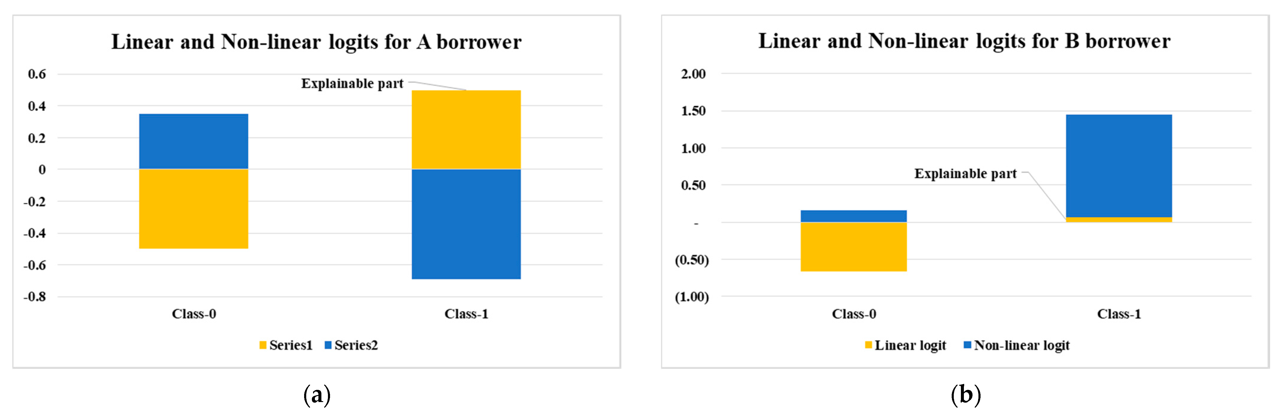
4.3. Model Interpretability

In this section, we show how to interpret the PIA-Soft model. As we explained, our model produces linear and non-linear logits for each borrower. Figure 3 shows the predicted linear and non-linear logits for A and B borrowers from German dataset. For A borrower, since the logit for class-1 is higher than class-0, we can predict that this borrower belongs to class-1. According to the proportion of class-1’s logit, the linear logit is larger than the non-linear logit, and we can only explain how the linear logit depends on the explanatory variables. In other words, we can explain and understand most of the borrower’s score for borrower A. On the contrary, for borrower B, the linear logit is a very small percentage of the total logit; therefore, we cannot explain the most of the borrower’s score. For this reason, our proposed PIA-Soft model can be partially interpretable. In terms of all datasets, the linear and non-linear logits for each borrower are show in Figure A1, Figure A2, Figure A3 and Figure A4.
In addition, our model can compute the impact on model output for each variable. Figure 3 shows the impact of variables for each class on German dataset. We can observe that if the amount of the most valuable available asset increases, the logit for class-0 (good borrower) increases more than the logit for class-1 (bad borrower). In other words, we can say that if the borrower has a large amount of valuable available assets, the borrower’s credit risk is decreased.
We also display how other variables affect credit score for all datasets in Figure 4 for German dataset. These estimated coefficients from the results of the PIA-Soft model are logically consistent with the real-life and logistic regression (see Figure 5). The logistic regression estimates coefficients for only class-1. Therefore, we compare weight parameters of the PIA-Soft model for class-1 to the logistic regression’s coefficients. We also displayed the impact of variables for each class and the comparison of PIA-Soft model and Logistic regression on other datasets in Figure A5, Figure A6, Figure A7, Figure A8, Figure A9 and Figure A10. In the end, our experimental results show that PIA-Soft model suggests a promising direction for partially interpretable machine learning model that can combine the softmax regression and neural network by end-to-end training.

5. Discussion

For credit scoring application, the model interpretability is one of the most critical features, and financial institutions want to understand how the borrower’s credit risk depends on the borrower’s characteristics. Recently, machine learning models have been successfully used to establish credit scoring models with high predictive performance. However, the machine learning model’s ambiguous decision-making process indicates the need to develop an explainable model with a high-predictive performance.
In this work, we aimed to propose an interpretable credit scoring model that can achieve state-of-the-art predictive performance using softmax regression and neural network models. Our proposed model consists of two main components: linear (softmax regression) and non-linear (neural network). The linear part explains the fundamental relationship between input and output variables. The non-linear part serves to improve the prediction performance by identifying the non-linear relationship between features for each borrower. In order to show the superiority of our proposed model, we compared our model to high-performance machine learning benchmarks on four public credit scoring datasets. In addition, in order to show our model can handle class imbalance problem without sampling techniques, we compare machine learning baselines with over sampling techniques. As bad borrowers occur infrequently, standard deep learning architectures tend to misclassify the minority (bad borrowers) classes compared to the majority (good borrowers) classes [11]. Therefore, we used the softmax function as an output of our model. Since the softmax computes the probability distributions of a list of potential outcomes and we update the logit (input of softmax function) for each class using neural network and linear models, our PIA-Soft model could handle the class imbalance problem.
Experimental results showed that our proposed model significantly outperformed machine learning models in terms of predictive performance. We also compare our proposed model to logistic regression to evaluate the model interpretation. From the result, the estimated coefficients of the PIA-Soft model are logically consistent with the real-life and logistic regression. Unlike logistic regression, our proposed model measures the impact of variables for each class, so we can estimate which class the borrower can move to faster based on each variable’s change. For example, the “the duration of credit” variable has an insignificant effect on class 1 (bad borrower) and a substantial impact on class 0 (good) for German dataset.
Finally, our proposed model suggests a promising direction for a partially interpretable machine learning model that can combine the softmax regression and neural network by end-to-end training.
However, since we use bank clients’ data to construct a credit scoring model, this sample data may differ from the overall population distribution. Therefore, there is a limitation that the trained machine learning models cannot be robust on overall population distribution. To solve this problem, we anticipate potential future work in this area that includes developing adaptive machine-learning algorithms for unseen data based on generative models such as variational auto-encoder, generative adversarial networks, etc.

6. Conclusions

In this work, we proposed a novel partially interpretable adaptive softmax regression model for class imbalance issue in the application of credit scoring. We compared our proposed model to benchmark machine learning models on four benchmark imbalanced credit scoring datasets. The results showed that our proposed PIA-Soft model significantly improved the baselines. We also observed that our model works better on both small and large datasets. In addition, we demonstrated that how our model partially interpret output. Depending on the characteristic of borrowers, our model logically explains the relationship between input and output. This marginal explanation between input and output can be used by financial institutions in their decision-making.

Author Contributions

L.M. and K.H.R. conceived the idea behind the paper. L.M. wrote the code for experiment. L.M. and O.-E.N. carried out the experiments and results. L.M., N.T.-U., O.-E.N., and K.H.R. drafted and revised the manuscript. All contributing authors have read and approved this manuscript prior to submission and agree to resolve any questions relating to any part of this paper. All authors have read and agreed to the published version of the manuscript.

Funding

This research was supported by the Basic Science Research Program through the National Research Foundation of Korea (NRF) funded by the Ministry of Science, ICT and Future Planning (No. 2019K2A9A2A06020672 and No. 2020R1A2B5B02001717).

Institutional Review Board Statement

Not applicable.

Informed Consent Statement

Not applicable.

Data Availability Statement

Not applicable.

Acknowledgments

This work has been done partially while Lkhagvadorj Munkhdalai visited in the Biomedical Engineering Institute, Chiang Mai University.

Conflicts of Interest

The authors declare no conflict of interest.

Appendix A

Figure A1. The predicted linear and nonlinear logits for each class on German dataset.
Applsci 11 03227 g0a1
Figure A2. The predicted linear and nonlinear logits for each class on Australian dataset.
Applsci 11 03227 g0a2
Figure A3. The predicted linear and nonlinear logits for each class on Taiwan dataset.
Applsci 11 03227 g0a3
Figure A4. The predicted linear and non-linear logits for each class on FICO dataset.
Applsci 11 03227 g0a4
Figure A5. The impact of variables for each class on Australian dataset.
Applsci 11 03227 g0a5
Figure A6. Comparison of PIA-Soft model and Logistic regression on Australian dataset.
Applsci 11 03227 g0a6
Figure A7. The impact of variables for each class on Taiwan dataset.
Applsci 11 03227 g0a7
Figure A8. Comparison of PIA-Soft model and Logistic regression on Taiwan dataset.
Applsci 11 03227 g0a8
Figure A9. The impact of variables for each class on FICO dataset.
Applsci 11 03227 g0a9
Figure A10. Comparison of PIA-Soft model and Logistic regression on FICO dataset.
Applsci 11 03227 g0a10

References

  1. Dastile, X.; Celik, T.; Potsane, M. Statistical and machine learning models in credit scoring: A systematic literature survey. Appl. Soft Comput. 2020, 91, 106263–106284. [Google Scholar] [CrossRef]
  2. Munkhdalai, L.; Munkhdalai, T.; Namsrai, O.E.; Lee, J.Y.; Ryu, K.H. An empirical comparison of machine-learning methods on bank client credit assessments. Sustainability 2019, 11, 699. [Google Scholar] [CrossRef] [Green Version]
  3. Demajo, L.M.; Vella, V.; Dingli, A. Explainable AI for Interpretable Credit Scoring. arXiv 2020, arXiv:2012.03749. [Google Scholar]
  4. Bussmann, N.; Giudici, P.; Marinelli, D.; Papenbrock, J. Explainable machine learning in credit risk management. Comput. Econ. 2020, 57, 203–216. [Google Scholar] [CrossRef]
  5. Došilović, F.K.; Brčić, M.; Hlupić, N. Explainable artificial intelligence: A survey. InMIPRO 2018, 41, 210–215. [Google Scholar]
  6. Modarres, C.; Ibrahim, M.; Louie, M.; Paisley, J. Towards explainable deep learning for credit lending: A case study. arXiv 2018, arXiv:1811.06471. [Google Scholar]
  7. Munkhdalai, L.; Wang, L.; Park, H.W.; Ryu, K.H. Advanced neural network approach, its explanation with lime for credit scoring application. InACIIDS 2019, 11432, 407–419. [Google Scholar]
  8. Brown, I.; Mues, C. An experimental comparison of classification algorithms for imbalanced credit scoring data sets. Expert Syst. Appl. 2012, 39, 3446–3453. [Google Scholar] [CrossRef] [Green Version]
  9. Marqués, A.I.; García, V.; Sánchez, J.S. On the suitability of resampling techniques for the class imbalance problem in credit scoring. J. Oper. Res. Soc. 2013, 64, 1060–1070. [Google Scholar] [CrossRef] [Green Version]
  10. Junior, L.M.; Nardini, F.M.; Renso, C.; Trani, R.; Macedo, J.A. A novel approach to define the local region of dynamic selection techniques in imbalanced credit scoring problems. Expert Syst. Appl. 2020, 152, 113351. [Google Scholar] [CrossRef]
  11. Munkhdalai, L.; Munkhdalai, T.; Ryu, K.H. GEV-NN: A deep neural network architecture for class imbalance problem in binary classification. Knowl. Based Syst. 2020, 194, 105534. [Google Scholar] [CrossRef]
  12. He, K.; Zhang, X.; Ren, S.; Sun, J. Deep residual learning for image recognition. In Proceedings of the IEEE Conference on Computer Vision and Pattern Recognition (CVPR), Las Vegas, NV, USA, 27–30 June 2016; pp. 770–778. [Google Scholar]
  13. Cox, D.R. The regression analysis of binary sequences. J. R. Stat. Soc. Ser. B Stat. Methodol. 1958, 20, 215–242. [Google Scholar] [CrossRef]
  14. Breiman, L. Random forests. Mach. Learn 2001, 45, 5–32. [Google Scholar] [CrossRef] [Green Version]
  15. Freund, Y.; Schapire, R.E. A decision-theoretic generalization of on-line learning and an application to boosting. J. Comput. Syst. Sci. 1997, 55, 119–139. [Google Scholar] [CrossRef] [Green Version]
  16. Chen, T.; Guestrin, C. Xgboost: A scalable tree boosting system. In Proceedings of the 22nd ACM Sigkdd International Conference on Knowledge Discovery and Data Mining, San Francisco, CA, USA, 13–17 August 2016; pp. 785–794. [Google Scholar]
  17. Rosenblatt, F. The perceptron: A probabilistic model for information storage and organization in the brain. Psychol. Rev. 1958, 65, 386. [Google Scholar] [CrossRef] [PubMed] [Green Version]
  18. Ke, G.; Meng, Q.; Finley, T.; Wang, T.; Chen, W.; Ma, W.; Liu, T.Y. Lightgbm: A highly efficient gradient boosting decision tree. NIPS 2017, 30, 3146–3154. [Google Scholar]
  19. Dorogush, A.V.; Ershov, V.; Gulin, A. CatBoost: Gradient boosting with categorical features support. arXiv 2018, arXiv:1810.11363. [Google Scholar]
  20. Arik, S.O.; Pfister, T. Tabnet: Attentive interpretable tabular learning. arXiv 2019, arXiv:1908.07442. [Google Scholar]
  21. Hand, D.J.; Anagnostopoulos, C. A better Beta for the H measure of classification performance. Pattern Recognit. Lett. 2014, 40, 41–46. [Google Scholar] [CrossRef] [Green Version]
  22. Lessmann, S.; Baesens, B.; Seow, H.V.; Thomas, L.C. Benchmarking state-of-the-art classification algorithms for credit scoring: An update of research. Eur. J. Oper. Res. 2015, 247, 124–136. [Google Scholar] [CrossRef] [Green Version]
  23. LeCun, Y.; Bengio, Y.; Hinton, G. Deep learning. Nature 2015, 521, 436–444. [Google Scholar] [CrossRef]
  24. Louzada, F.; Ara, A.; Fernandes, G.B. Classification methods applied to credit scoring: Systematic review and overall comparison. Comput. Oper. Res. 2016, 21, 117–134. [Google Scholar] [CrossRef] [Green Version]
  25. Orgler, Y.E. A credit scoring model for commercial loans. J. Money Credit. Bank 1970, 2, 435–445. [Google Scholar] [CrossRef]
  26. Bellotti, T.; Crook, J. Support vector machines for credit scoring and discovery of significant features. Expert Syst. Appl. 2009, 36, 3302–3308. [Google Scholar] [CrossRef] [Green Version]
  27. Ala’raj, M.; Abbod, M.F. Classifiers consensus system approach for credit scoring. Knowl. Based Syst. 2016, 104, 89–105. [Google Scholar] [CrossRef]
  28. Chuang, C.L.; Huang, S.T. A hybrid neural network approach for credit scoring. Expert Syst. 2011, 28, 185–196. [Google Scholar] [CrossRef]
  29. Munkhdalai, L.; Lee, J.Y.; Ryu, K.H. A Hybrid Credit Scoring Model Using Neural Networks and Logistic Regression. In Advances in Intelligent Information Hiding and Multimedia Signal Processing; Springer: Singapore, 2020; pp. 251–258. [Google Scholar]
  30. Vellido, A.; Martín-Guerrero, J.D.; Lisboa, P.J. Making machine learning models interpretable. InESANN 2012, 12, 163–172. [Google Scholar]
  31. West, D. Neural network credit scoring models. Comput. Oper. Res. 2000, 27, 1131–1152. [Google Scholar] [CrossRef]
  32. Pang, S.L. Study on Credit Scoring Model and Forecasting Based on Probabilistic Neural Network. Syst. Eng. Theory. Pract. 2005, 5, 006. [Google Scholar]
  33. Lisboa, P.J.; Etchells, T.A.; Jarman, I.H.; Arsene, C.T.; Aung, M.H.; Eleuteri, A.; Biganzoli, E. Partial logistic artificial neural network for competing risks regularized with automatic relevance determination. IEEE Trans. Neural Netw. 2009, 20, 1403–1416. [Google Scholar] [CrossRef]
  34. Marcano-Cedeño, A.; Quintanilla-Domínguez, J.; Andina, D. WBCD breast cancer database classification applying artificial metaplasticity neural network. Expert Syst. Appl. 2011, 38, 9573–9579. [Google Scholar] [CrossRef]
  35. Abdou, H.; Pointon, J.; El-Masry, A. Neural nets versus conventional techniques in credit scoring in Egyptian banking. Expert Syst. Appl. 2008, 35, 1275–1292. [Google Scholar] [CrossRef] [Green Version]
  36. Ala’raj, M.; Abbod, M.F. A new hybrid ensemble credit scoring model based on classifiers consensus system approach. Expert Syst. Appl. 2016, 64, 36–55. [Google Scholar] [CrossRef]
  37. Xiao, H.; Xiao, Z.; Wang, Y. Ensemble classification based on supervised clustering for credit scoring. Appl. Soft Comput. 2016, 43, 73–86. [Google Scholar] [CrossRef]
  38. Shen, F.; Zhao, X.; Kou, G.; Alsaadi, F.E. A new deep learning ensemble credit risk evaluation model with an improved synthetic minority oversampling technique. Appl. Soft Comput. 2021, 98, 106852. [Google Scholar] [CrossRef]
  39. He, H.; Zhang, W.; Zhang, S. A novel ensemble method for credit scoring: Adaption of different imbalance ratios. Expert Syst. Appl. 2018, 98, 105–117. [Google Scholar] [CrossRef]
  40. Zhang, W.; Yang, D.; Zhang, S.; Ablanedo-Rosas, J.H.; Wu, X.; Lou, Y. A novel multi-stage ensemble model with enhanced outlier adaptation for credit scoring. Expert Syst. Appl. 2021, 165, 113872. [Google Scholar] [CrossRef]
  41. Ribeiro, M.T.; Singh, S.; Guestrin, C. “Why should i trust you?” Explaining the predictions of any classifier. In Proceedings of the 22nd ACM SIGKDD International Conference on Knowledge Discovery and Data Mining, San Francisco, CA, USA, 13–17 August 2016; pp. 1135–1144. [Google Scholar]
  42. Lundberg, S.; Lee, S.I. A unified approach to interpreting model predictions. arXiv 2017, arXiv:1705.07874. [Google Scholar]
  43. Torrent, N.L.; Visani, G.; Bagli, E. PSD2 Explainable AI Model for Credit Scoring. arXiv 2020, arXiv:2011.10367. [Google Scholar]
  44. Munkhdalai, L.; Munkhdalai, T.; Ryu, K.H. A locally adaptive interpretable regression. arXiv 2020, arXiv:2005.03350. [Google Scholar]
  45. Ariza-Garzón, M.J.; Arroyo, J.; Caparrini, A.; Segovia-Vargas, M.J. Explainability of a machine learning granting scoring model in peer-to-peer lending. IEEE Access 2020, 8, 64873–64890. [Google Scholar] [CrossRef]
  46. FICO Explainable Machine Learning Challenge. Available online: https://community.fico.com/community/xml (accessed on 24 January 2021).
  47. Dash, S.; Günlük, O.; Wei, D. Boolean decision rules via column generation. arXiv 2018, arXiv:1805.09901. [Google Scholar]
  48. Bracke, P.; Datta, A.; Jung, C.; Sen, S. Machine learning explainability in finance: An application to default risk analysis. Bank Engl. Staff Work Paper 2019, 816, 1–44. [Google Scholar] [CrossRef] [Green Version]
  49. Chen, L.; Zhou, M.; Su, W.; Wu, M.; She, J.; Hirota, K. Softmax regression based deep sparse autoencoder network for facial emotion recognition in human-robot interaction. Inf. Sci. 2018, 428, 49–61. [Google Scholar] [CrossRef]
  50. Asuncion, A.; Newman, D. UCI Machine Learning Repository. Available online: https://archive.ics.uci.edu/ml/index.php (accessed on 24 January 2021).
  51. Chawla, N.V.; Bowyer, K.W.; Hall, L.O.; Kegelmeyer, W.P. SMOTE: Synthetic Minority Over-Sampling Technique. J. Artif. Intell. Res. 2002, 16, 321–357. [Google Scholar] [CrossRef]
  52. He, H.; Bai, Y.; Garcia, E.A.; Li, S. ADASYN: Adaptive synthetic sampling approach for imbalanced learning. In Proceedings of the 2008 IEEE International Joint Conference on Neural Networks, Hong Kong, China, 1–8 June 2008; pp. 1322–1328. [Google Scholar]
  53. Batista, G.E.; Prati, R.C.; Monard, M.C. A study of the behavior of several methods for balancing machine learning training data. ACM SIGKDD 2004, 6, 20–29. [Google Scholar] [CrossRef]
Figure 1. Partially interpretable adaptive softmax (PIA-Soft) architecture: where x . is an input, and p 0 and p 1 . are the predicted probabilities of the first and second classes, respectively.
Applsci 11 03227 g001
Figure 2. Overall architecture of PIA-Soft model.
Applsci 11 03227 g002
Figure 3. Linear and nonlinear logits for A and B borrowers from German dataset, (a) figure shows linear and nonlinear logits for A borrower and (b) figure shows linear and nonlinear logits for B borrower.
Applsci 11 03227 g003
Figure 4. Comparison of PIA-Soft model and Logistic regression on German dataset.
Applsci 11 03227 g004
Figure 5. The impact of variables for each class on German dataset.
Applsci 11 03227 g005
Table 1. Summary of datasets.
DatasetInstancesVariablesGood/Bad
German100024700/300
Australian69014387/307
Taiwan6000233000/3000
FICO9871245136/4735
Table 2. Searching space of hyper-parameters.
ModelParametersSearch Space
Random Forestmax_depth(2, 8)
min_samples_split(1, 8)
min_samples_leaf(1, 8]
criterion{‘gini’, ‘entropy’}
bootstrap{True, False}
AdaBoostlearning_rate(0.1, 1)
algorithm{‘SAMME.R’, ‘SAMME’}
XGBoostmin_child_weight(1, 10)
gamma{0, 0.1, 0.5, 0.8, 1}
subsample{0.5, 0.75, 0.9}
colsample_bytree{0.5, 0.6, 0.7, 0.8, 0.9, 1}
max_depth{2, 8}
learning_rate{0.01, 0.1, 0.2, 0.3, 0.5}
LightGBMmin_child_samples(10, 60)
reg_alpha{0, 0.1, 0.5, 0.8, 1}
subsample{0.5, 0.75, 0.9}
colsample_bytree{0.5, 0.6, 0.7, 0.8, 0.9, 1}
max_depth(2, 8)
learning_rate{0.01, 0.1, 0.2, 0.3, 0.5}
CatBoostmin_child_samples(10, 60)
subsample{0.5, 0.75, 0.9}
colsample_bytree{0.5, 0.6, 0.7, 0.8, 0.9, 1}
max_depth(2, 8)
learning_rate{0.01, 0.1, 0.2, 0.3, 0.5}
TabNetn_d(4, 16)
n_a(4, 16)
mask_type{‘entmax’, ‘sparsemax’}
Table 3. The prediction performance for German dataset over different evaluation metrics.
Sampling MethodModelAUCAccuracyF-SscoreG-Mean
No samplingLogistic0.788 +/− 0.0720.762 +/− 0.0620.774 +/− 0.0560.777 +/− 0.053
Random forest0.788 +/− 0.0710.771 +/− 0.0700.783 +/− 0.0650.778 +/− 0.067
AdaBoost0.762 +/− 0.0380.721 +/− 0.0400.736 +/− 0.0410.737 +/− 0.039
XGBoost0.778 +/− 0.0590.762 +/− 0.0590.775 +/− 0.0510.774 +/− 0.053
Neural Network0.791 +/− 0.0690.759 +/− 0.0610.771 +/− 0.0540.775 +/− 0.053
LightGBM0.766 +/− 0.0220.764 +/− 0.0190.777 +/− 0.0180.773 +/− 0.023
CatBoost0.783 +/− 0.0180.771 +/− 0.0280.783 +/− 0.0230.775 +/− 0.023
TabNet0.653 +/− 0.0220.678 +/− 0.0180.695 +/− 0.0200.685 +/− 0.016
SMOTELogistic0.798 +/− 0.0150.767 +/− 0.0120.767 +/− 0.0120.767 +/− 0.012
Random forest0.776 +/− 0.0250.752 +/− 0.0230.754 +/− 0.0180.753 +/− 0.020
AdaBoost0.725 +/− 0.0190.715 +/− 0.0210.715 +/− 0.0210.715 +/− 0.020
XGBoost0.782 +/− 0.0290.750 +/− 0.0440.752 +/− 0.0360.751 +/− 0.042
Neural Network0.795 +/− 0.0200.764 +/− 0.0190.765 +/− 0.0140.765 +/− 0.015
LightGBM0.763 +/− 0.0410.758 +/− 0.0430.771 +/− 0.0410.764 +/− 0.042
CatBoost0.775 +/− 0.0390.759 +/− 0.0580.772 +/− 0.0540.770 +/− 0.053
TabNet0.717 +/− 0.0390.720 +/− 0.0430.735 +/− 0.0370.727 +/− 0.038
ADASYNLogistic0.794 +/− 0.0670.788 +/− 0.0550.799 +/− 0.0510.797 +/− 0.054
Random forest0.793 +/− 0.0700.773 +/− 0.0580.785 +/− 0.0500.783 +/− 0.055
AdaBoost0.715 +/− 0.0420.703 +/− 0.0480.719 +/− 0.0450.716 +/− 0.043
XGBoost0.765 +/− 0.0750.764 +/− 0.0580.776 +/− 0.0520.772 +/− 0.054
Neural Network0.796 +/− 0.0640.792 +/− 0.0590.802 +/− 0.0560.800 +/− 0.056
LightGBM0.758 +/− 0.0240.742 +/− 0.0380.756 +/− 0.0360.749 +/− 0.037
CatBoost0.780 +/− 0.0380.774 +/− 0.0380.786 +/− 0.0360.778 +/− 0.037
TabNet0.709 +/− 0.0750.711 +/− 0.0770.726 +/− 0.0720.720 +/− 0.073
ROSLogistic0.786 +/− 0.0710.766 +/− 0.0710.778 +/− 0.0670.780 +/− 0.065
Random forest0.797 +/− 0.0680.764 +/− 0.0840.777 +/− 0.0770.779 +/− 0.077
AdaBoost0.710 +/− 0.0500.688 +/− 0.0520.704 +/− 0.0520.710 +/− 0.045
XGBoost0.769 +/− 0.0680.748 +/− 0.0780.761 +/− 0.0700.764 +/− 0.065
Neural Network0.788 +/− 0.0670.749 +/− 0.0470.761 +/− 0.0430.761 +/− 0.043
LightGBM0.793 +/− 0.0140.767 +/− 0.0130.767 +/− 0.0130.767 +/− 0.013
CatBoost0.794 +/− 0.0130.767 +/− 0.0100.767 +/− 0.0100.766 +/− 0.010
TabNet0.780 +/− 0.0140.760 +/− 0.0140.760 +/− 0.0150.759 +/− 0.014
PIA-Soft (Ours)0.798 +/− 0.0450.781 +/− 0.0510.795 +/− 0.0470.795 +/− 0.049
Table 4. The prediction performance for Australia dataset over different evaluation metrics.
Sampling MethodModelAUCAccuracyF-ScoreG-Mean
No samplingLogistic0.911 +/− 0.0530.869 +/− 0.0470.868 +/− 0.0470.862 +/− 0.046
Random forest0.916 +/− 0.0640.883 +/− 0.0530.883 +/− 0.0520.876 +/− 0.052
AdaBoost0.928 +/− 0.0350.894 +/− 0.0240.894 +/− 0.0230.891 +/− 0.024
XGBoost0.915 +/− 0.0590.870 +/− 0.0670.870 +/− 0.0680.868 +/− 0.065
Neural Network0.904 +/− 0.0520.867 +/− 0.0510.866 +/− 0.0510.860 +/− 0.049
LightGBM0.937 +/− 0.0220.904 +/− 0.0210.904 +/− 0.0210.902 +/− 0.022
CatBoost0.938 +/− 0.0150.910 +/− 0.0180.910 +/− 0.0180.907 +/− 0.017
TabNet0.852 +/− 0.0470.823 +/− 0.0340.822 +/− 0.0340.816 +/− 0.038
SMOTELogistic0.910 +/− 0.0540.873 +/− 0.0560.873 +/− 0.0560.867 +/− 0.056
Random forest0.916 +/− 0.0650.884 +/− 0.0560.884 +/− 0.0560.882 +/− 0.055
AdaBoost0.923 +/− 0.0390.879 +/− 0.0450.879 +/− 0.0450.876 +/− 0.044
XGBoost0.903 +/− 0.0580.855 +/− 0.0600.854 +/− 0.0610.848 +/− 0.060
Neural Network0.906 +/− 0.0540.842 +/− 0.1090.826 +/− 0.1550.834 +/− 0.117
LightGBM0.936 +/− 0.0250.898 +/− 0.0230.898 +/− 0.0230.897 +/− 0.023
CatBoost0.931 +/− 0.0190.914 +/− 0.0190.914 +/− 0.0190.912 +/− 0.018
TabNet0.836 +/− 0.0230.821 +/− 0.0300.822 +/− 0.0310.820 +/− 0.031
ADASYNLogistic0.911 +/− 0.0530.876 +/− 0.0510.876 +/− 0.0510.870 +/− 0.050
Random forest0.917 +/− 0.0650.880 +/− 0.0550.880 +/− 0.0540.875 +/− 0.054
AdaBoost0.916 +/− 0.0390.873 +/− 0.0390.873 +/− 0.0390.871 +/− 0.038
XGBoost0.917 +/− 0.0600.851 +/− 0.1030.835 +/− 0.1470.841 +/− 0.122
Neural Network0.904 +/− 0.0540.863 +/− 0.0460.863 +/− 0.0460.859 +/− 0.045
LightGBM0.934 +/− 0.0230.898 +/− 0.0150.898 +/− 0.0150.896 +/− 0.016
CatBoost0.934 +/− 0.0180.904 +/− 0.0160.904 +/− 0.0160.901 +/− 0.015
TabNet0.800 +/− 0.0630.804 +/− 0.0580.804 +/− 0.0580.801 +/− 0.057
ROSLogistic0.911 +/− 0.0530.879 +/− 0.0520.878 +/− 0.0520.872 +/− 0.052
Random forest0.917 +/− 0.0650.883 +/− 0.0550.883 +/− 0.0550.878 +/− 0.055
AdaBoost0.912 +/− 0.0450.862 +/− 0.0620.861 +/− 0.0630.859 +/− 0.061
XGBoost0.909 +/− 0.0670.857 +/− 0.0520.855 +/− 0.0520.849 +/− 0.052
Neural Network0.903 +/− 0.0550.846 +/− 0.0960.833 +/− 0.1320.835 +/− 0.117
LightGBM0.926 +/− 0.0260.892 +/− 0.0240.892 +/− 0.0240.891 +/− 0.024
CatBoost0.924 +/− 0.0120.902 +/− 0.0180.902 +/− 0.0190.900 +/− 0.018
TabNet0.842 +/− 0.0480.802 +/− 0.0590.803 +/− 0.0580.802 +/− 0.059
PIA-Soft (Ours)0.934 +/− 0.0410.896 +/− 0.0790.894 +/− 0.0860.895 +/− 0.075
Table 5. The prediction performance for Taiwan dataset over different evaluation metrics.
Sampling MethodModelAUCAccuracyF-ScoreG-Mean
No samplingLogistic0.637 +/− 0.0280.644 +/− 0.0250.644 +/− 0.0250.643 +/− 0.024
Random forest0.750 +/− 0.0160.732 +/− 0.0120.732 +/− 0.0120.732 +/− 0.012
AdaBoost0.721 +/− 0.0100.708 +/− 0.0150.708 +/− 0.0150.708 +/− 0.015
XGBoost0.744 +/− 0.0190.724 +/− 0.0160.724 +/− 0.0160.725 +/− 0.016
Neural Network0.736 +/− 0.0180.715 +/− 0.0180.715 +/− 0.0180.715 +/− 0.018
LightGBM0.751 +/− 0.0110.732 +/− 0.0120.731 +/− 0.0120.731 +/− 0.012
CatBoost0.753 +/− 0.0110.734 +/− 0.0120.734 +/− 0.0120.734 +/− 0.012
TabNet0.739 +/− 0.0120.723 +/− 0.0190.723 +/− 0.0180.723 +/− 0.018
PIA-Soft (Ours)0.744 +/− 0.0150.725 +/− 0.0150.726 +/− 0.0150.726 +/− 0.015
Table 6. The prediction performance for FICO dataset over different evaluation metrics.
Sampling MethodModelAUCAccuracyF-ScoreG-Mean
No samplingLogistic0.798 +/− 0.0150.767 +/− 0.0120.767 +/− 0.0120.767 +/− 0.012
Random forest0.774 +/− 0.0300.755 +/− 0.0160.757 +/− 0.0140.755 +/− 0.016
AdaBoost0.773 +/− 0.0160.755 +/− 0.0140.755 +/− 0.0140.755 +/− 0.014
XGBoost0.787 +/− 0.0180.754 +/− 0.0350.756 +/− 0.0290.757 +/− 0.025
Neural Network0.798 +/− 0.0140.756 +/− 0.0350.758 +/− 0.0280.760 +/− 0.025
LightGBM0.792 +/− 0.0150.766 +/− 0.0140.766 +/− 0.0140.766 +/− 0.014
CatBoost0.795 +/− 0.0140.768 +/− 0.0100.768 +/− 0.0100.768 +/− 0.010
TabNet0.782 +/− 0.0130.760 +/− 0.0100.760 +/− 0.0100.760 +/− 0.010
SMOTELogistic0.798 +/− 0.0150.767 +/− 0.0120.767 +/− 0.0120.767 +/− 0.012
Random forest0.776 +/− 0.0250.752 +/− 0.0230.754 +/− 0.0180.753 +/− 0.020
AdaBoost0.725 +/− 0.0190.715 +/− 0.0210.715 +/− 0.0210.715 +/− 0.020
XGBoost0.782 +/− 0.0290.750 +/− 0.0440.752 +/− 0.0360.751 +/− 0.042
Neural Network0.795 +/− 0.0200.764 +/− 0.0190.765 +/− 0.0140.765 +/− 0.015
LightGBM0.792 +/− 0.0140.766 +/− 0.0140.766 +/− 0.0140.766 +/− 0.014
CatBoost0.794 +/− 0.0140.767 +/− 0.0120.767 +/− 0.0120.767 +/− 0.011
TabNet0.786 +/− 0.0160.763 +/− 0.0130.763 +/− 0.0130.763 +/− 0.013
ADASYNLogistic0.798 +/− 0.0150.767 +/− 0.0120.767 +/− 0.0120.767 +/− 0.012
Random forest0.773 +/− 0.0330.751 +/− 0.0250.753 +/− 0.0200.751 +/− 0.025
AdaBoost0.727 +/− 0.0280.718 +/− 0.0180.718 +/− 0.0180.718 +/− 0.018
XGBoost0.781 +/− 0.0320.754 +/− 0.0350.756 +/− 0.0290.755 +/− 0.032
Neural Network0.795 +/− 0.0210.764 +/− 0.0180.766 +/− 0.0130.766 +/− 0.014
LightGBM0.792 +/− 0.0150.766 +/− 0.0140.766 +/− 0.0140.766 +/− 0.014
CatBoost0.795 +/− 0.0140.768 +/− 0.0100.768 +/− 0.0100.768 +/− 0.010
TabNet0.783 +/− 0.0160.759 +/− 0.0140.759 +/− 0.0140.759 +/− 0.014
ROSLogistic0.798 +/− 0.0150.767 +/− 0.0120.767 +/− 0.0120.767 +/− 0.012
Random forest0.781 +/− 0.0180.755 +/− 0.0220.757 +/− 0.0180.755 +/− 0.023
AdaBoost0.725 +/− 0.0160.714 +/− 0.0140.714 +/− 0.0140.714 +/− 0.014
XGBoost0.786 +/− 0.0190.750 +/− 0.0470.752 +/− 0.0400.755 +/− 0.029
Neural Network0.799 +/− 0.0150.761 +/− 0.0220.763 +/− 0.0170.763 +/− 0.017
LightGBM0.793 +/− 0.0140.767 +/− 0.0130.767 +/− 0.0130.767 +/− 0.013
CatBoost0.794 +/− 0.0130.767 +/− 0.0100.767 +/− 0.0100.766 +/− 0.010
TabNet0.780 +/− 0.0140.760 +/− 0.0140.760 +/− 0.0150.759 +/− 0.014
PIA-Soft (Ours)0.807 +/− 0.0160.788 +/− 0.0130.788 +/− 0.0130.788 +/− 0.013
Publisher’s Note: MDPI stays neutral with regard to jurisdictional claims in published maps and institutional affiliations.

