Online Forecasting and Anomaly Detection Based on the ARIMA Model

Abstract

Real-time diagnostics of complex technical systems such as power plants are critical to keep the system in its working state. An ideal diagnostic system must detect any fault in advance and predict the future state of the technical system, so predictive algorithms are used in the diagnostics. This paper proposes a novel, computationally simple algorithm based on the Auto-Regressive Integrated Moving Average model to solve anomaly detection and forecasting problems. The good performance of the proposed algorithm was confirmed in numerous numerical experiments for both anomaly detection and forecasting problems. Moreover, a description of the Autoregressive Integrated Moving Average Fault Detection (ARIMAFD) library, which includes the proposed algorithms, is provided in this paper. The developed algorithm proves to be an efficient algorithm and can be applied to problems related to anomaly detection and technological parameter forecasting in real diagnostic systems.

1. Introduction

The number of real-time or online applications that generate time series data is increasing rapidly in various industries. The importance of anomaly detection in such applications is also increasing [1]. Generally, anomaly detection algorithms are intended to find a point of change in the system’s state or behavior. The traditional classification of anomaly detection algorithms includes “online” and “offline” types. The main difference between them is that the offline data availability problem assumes that the full set of data is available, transforming the problem by finding all existing changepoints accurately. The online problem, in turn, expects the data to become available point by point in real time, transforming the problem by finding anomalies as soon as they occur [2]. Online or streaming applications are mainly used in critical systems where real-time decisions with acceptable quality are required. The trade-off between the detector’s quality and computational time is one of the challenges for online algorithms. The problems that can be solved using these algorithms are actually important and vary from computer network intrusions to heart attack recognition.

The Autoregressive Moving Average (ARMA) model is widely used for time series analysis and forecasting [3,4,5]. The ARMA model is a combination of the Autoregressive model (AR), which describes the analytical component of the signal, and the moving average model (MA), which describes the noise component of the signal. The advantage of the ARMA model is its clear mathematical and statistical base. However, there are serious drawbacks such as time-consuming model tuning and hyperparameter selection. Another disadvantage of the model is its applicability only to stationary time series. The latter problem is resolved with the Autoregressive Integrated Moving Average (ARIMA) model, which evaluates the differences in the time series. A number of studies have been carried out for the automatic selection of hyperparameters; however, the need for manual selection of hyperparameters remains [6]. ARMA and ARIMA models and their modifications, such as Seasonal Autoregressive Integrated Moving Average (SARIMA), are described in detail in [6,7,8].

Since the state of systems can gradually change over time, causing data drifts or statistical changes in the data, continuous updating of the model is required to achieve the correct results and to make the model more robust and adaptive [9]. As such, continuous model learning or online refitting is used in many applications and can be achieved in a wide variety of practical tasks, such as predicting the values of technological parameters and detecting equipment faults [10]. Unfortunately, training the classical ARIMA models with a large amount of data is time consuming, making it inefficient to use and refit the model in the online mode. Many works are dedicated to creating online ARIMA algorithms for forecasting problems (see [11,12,13,14,15,16,17]). Most of them are based on removing the terms of the moving average and increasing the order of the auto-regressive part.

In this paper, a comparison of several online algorithms based on the ARIMA model is provided. Moreover, this paper represents a new algorithm that can be used both for anomaly detection and forecasting purposes in real-time streaming applications. Numerical experiments were conducted on the Numenta Anomaly Benchmark (NAB) [9], which contains anomalous data from real-world streaming applications and a real-world proprietary turbogenerator-bearing vibration dataset. All proposed algorithms are implemented in the library in the Python3 programming language. A brief description of the library and a link to the source code can be found in the Materials and Methods section.

2. Materials and Methods

2.1. Classical ARIMA Model

The ARMA model is described by an equation from [6]:

$$\widehat{X_t}=\sum _{i=1}^q{\beta }_i{ϵ}_{t-i}+\sum _{i=1}^p{\alpha }_i{X}_{t-i}+{ϵ}_t+c$$

(1)

where $X_t$ is the value of the X time series at moment t; $\alpha \in {\mathbb{R}}^p$ and $\beta \in {\mathbb{R}}^q$ are the vectors of the weight coefficients; $ϵ$ is a noise term; c is a constant; ${\sum }_{i=1}^p{\alpha }_i{X}_{t-i}+{ϵ}_t+c$ is an autoregressive model with order p, which is a linear combination of the previous p values of series, constants and noise terms; ${\sum }_{i=1}^q{\beta }_i{ϵ}_{t-i}+{ϵ}_t$ is the moving average model with order q, which is a linear combination of the previous q noise terms and current noise term.

Time series representing real-world processes are often non-stationary. Deterministic components, such as trends, seasonality, slow and fast variation, and cyclical irregularity are usually represented in this manner. An effective way to remove most of these components is to compute their differences. For the time series X, at time moment t, the first order differences (lag = 1) are equal to $\nabla X_t=X_t-X_{t-1}$, while the second order differences are equal to ${\nabla }^2{X}_t=\nabla X_t-\nabla X_{t-1}$. To remove the seasonality, seasonal differences can be calculated, which are pairwise differences in values in neighboring seasons.

If ${\nabla }^d{X}_t$ is described by the ARMA model (p, q), it can be said that $X_t$ is described by the ARIMA model (p, d, q):

$${\nabla }^d{\tilde{X}}_t=\sum _{i=1}^q{\beta }_i{ϵ}_{t-i}+\sum _{i=1}^p{\alpha }_i{\nabla }^d{X}_{t-i}+{ϵ}_t+c$$

(2)

where p, d, q are the hyperparameters or orders of a model, $\alpha \in {\mathbb{R}}^p$ and $\beta \in {\mathbb{R}}^q$ are the vectors of the weight coefficients.

The predicted value of ${\tilde{X}}_t$ can be calculated as:

$${\tilde{X}}_t={\nabla }^d{\tilde{X}}_t+\sum _{i=0}^{d-1}{\nabla }^i{X}_{t-1}$$

(3)

As stated earlier, hyperparameter selection is a separate, non-trivial task. The Box–Jenkins method for solving this problem is described in [6].

2.2. Online Algorithms Based on the ARIMA Model

2.2.1. Online Gradient Descent

Generally, the maximum likelihood (ML) and prediction error (PE) methods with a non-convex error criterion function are used to find the optimal ARMA weights. Other algorithms (interested readers are directed to [18]) are also used to solve this problem, but they all have their drawbacks. For example, they may fail to deliver the global optima.

The use of classical online algorithms with convex optimization methods, in this case, is impossible since the moving average model is nonlinear in its parameters and, therefore, to estimate the parameters, it is necessary to use nonlinear estimation procedures [6]. In turn, noise components ${\left\{{ϵ}_t\right\}}_{t=1}^T$ are required at each iteration when updating the model weights $(\alpha ,\beta )$ and at each iteration of the prediction procedure.

The solution to this problem may be the ARMA Online Gradient Descent algorithm (ARMA-OGD) from [12] (see Algorithm 1, where $TL{M}_{max}q$ is the maximum value of the Lagrange multipliers [12]). In this case, all terms of an MA model are replaced by additional autoregressive terms. The ARIMA model (p, d, q) is converted to the ARIMA model (p + m, d, 0), where $m\in \mathbb{N}$ is a constant, meaning that the algorithm with the coefficient vector $\gamma \in {\mathbb{R}}^{p+m}$ attains a sublinear regret bound against the best ARMA model (p, d, q) prediction in hindsight, with weak assumptions of the noise terms. The sublinear regret with computational simplicity indicates the acceptableness of this approach. However, this algorithm requires the following assumptions:

• Noise components are randomly and independently distributed with zero expectations and satisfy the following conditions: $\mathbb{E}\left[\left|{ϵ}_t\right|\right]<M_{max}<\infty$ and $\mathbb{E}\left[{\ell }_t\left(X_t,X_t-{ϵ}_t\right)\right]<\infty$ for every t.
• The loss function ${\ell }_t$ must satisfy a Lipschitz condition [19].
• Autoregressive weight coefficients ${\alpha }_i$ satisfy $\left|{\alpha }_i\right|<1$. This assumption is necessary to restrict the decision set [12], but it is not necessary or sufficient for stability. In fact, the absolute values of autoregressive weight coefficients can be bounded to any other real number.
• Moving average weight coefficients ${\beta }_i$ satisfy ${\sum }_{i=1}^q\left|{\beta }_i\right|<1-\epsilon$ for some $\epsilon >0$.
• The signal is bounded by the constant. Without the loss of generality, we assume that $\left|X_t\right|<1$ for every t.

Algorithm 1 Online Gradient Descent.

Input Hyperparameters $p,d,q$, learning rate $\eta$; Set $m={log}_{max}\left({\left(TL{M}_{max}q\right)}^{-1}\right)$ For t from 1 to $T-1$ do:      Predict ${\tilde{X}}_t\left({\gamma }^t\right)={\sum }_{i=1}^{p+m}{\gamma }_i{\nabla }^d{X}_{t-i}+{\sum }_{i=0}^{d-1}{\nabla }^i{X}_{t-1}$;      Get $X_t$ and ${\ell }_t^m\left({\gamma }^t\right)={\ell }_t\left(X_t,{\tilde{X}}_t\left({\gamma }^t\right)\right)$;      Set ${\nabla }_t=\nabla {\ell }_t^m\left({\gamma }^t\right)$;      Update ${\gamma }^{t+1}\leftarrow {\prod }_{\mathcal{K}}\left({\gamma }^t-\frac{1}{\eta }{\nabla }_t\right)$ End for

2.2.2. Full Refitting

The next online algorithm considered, based on the ARIMA model, is a full refitting algorithm. In this algorithm, the model is refitted on the whole dataset, including new data, each time the new point(s) have been received (Algorithm 2). The “warm start” technology was used, according to which the weight coefficients of the ARIMA model are not initialized randomly, but are remembered from the last loop and are given as initials for a new fitting loop. This allows the optimization algorithm to converge much faster.

Algorithm 2 Full refitting.

Input Hyperparameters $p,d,q$, learning rate $\eta$; Set randomly ${\alpha }^1,{\beta }^1$ For t from $T_{test}^1$to$T-1$ do:      Set ${\alpha }^t,{\beta }^t\leftarrow fit{({\alpha }^{t-1},{\beta }^{t-1},[X_1\dots X_t],\eta )}^{*},$      Predict ${\tilde{X}}_t\left({\alpha }^t,{\beta }^t\right)={\sum }_{i=0}^{d-1}{\nabla }^i{X}_{t-1}+{\sum }_{i=1}^q{\beta }_i^t{ϵ}_{t-i}+{\sum }_{i=1}^p{\alpha }_i^t{\nabla }^d{X}_{t-i}+{ϵ}_t+c$ End for * $fit\left(\right)$ is the notation of any suitable optimization algorithm using “warm start” technology

2.2.3. Window Refitting

In the window refitting algorithm, the model is refitted not on the whole dataset, but only on its last section in relation to the current time moment. The size of each new training set is determined by the width of the window. The width is a hyperparameter, which requires an individual setting. The wider the window, the more accurate and computationally complex the model, and vice versa. This algorithm also uses “warm start” technology (see Algorithm 3).

Algorithm 3 Window refitting.

Input Hyperparameters $p,d,q$, learning rate $\eta$, window width W; Set randomly ${\alpha }^1,{\beta }^1$ For t from $T_{test}^1$to$T-1$ do:      Set ${\alpha }^t,{\beta }^t\leftarrow fit{({\alpha }^{t-1},{\beta }^{t-1},[X_{t-W}\dots X_t],\eta )}^{*},$      Predict ${\tilde{X}}_t\left({\alpha }^t,{\beta }^t\right)={\sum }_{i=0}^{d-1}{\nabla }^i{X}_{t-1}+{\sum }_{i=1}^q{\beta }_i^t{ϵ}_{t-i}+{\sum }_{i=1}^p{\alpha }_i^t{\nabla }^d{X}_{t-i}+{ϵ}_t+c$ End for * $fit\left(\right)$ is the notation of any suitable optimization algorithm using “warm start” technology

2.3. Performance Metric for the Forecasting Problem

To evaluate the forecasting algorithms, the Mean Absolute Percentage Error was used (Equation (4)). The main motivation for choosing this metric is the easy interpretability of the results and the ability to compare forecast errors between different physical measures.

$$MAPE(X_t,{\tilde{X}}_t)=\frac{1}{T}\sum _{t=1}^T\frac{\left|X_t-{\tilde{X}}_t\right|}{max\left(ϵ,\left|X_t\right|\right)}$$

(4)

where ${\tilde{X}}_t$ is a predicted value at a time moment t, $X_t$ is a true value at time moment t, T is the number of points in time series X, and $ϵ$ is an arbitrarily small yet strictly positive number to avoid undefined results when $X_t$ is zero—in our case, $ϵ=2.22·{10}^{-16}$.

2.4. Anomaly Detection Algorithms

2.4.1. Novel Anomaly Detection Algorithm Based on OGD Algorithm

According to the definition in [20], the technical state is the state of the system at a certain point in time, which, under certain environmental conditions, is characterized by the values of the parameters established by the technical documentation for the system. In our case, this is $X_t$. This state may implicitly include information about the presence of a defect or other anomaly in a system. Applying the ARIMA models to these parameters can make the presence of an anomaly in a technical system more apparent. Weight coefficients can provide more transparent and precise information about changes in a system state than the parameters themselves.

The Online Gradient Descent algorithm allows us to track weight coefficients in online mode. This makes it possible to use the base of the Online Gradient Descent algorithm not only for forecasting problems, but also for anomaly detection problems. For this, it is necessary to transform the OGD algorithm by essentially creating a novel algorithm based on it.

Let us suppose that we have the entire history of the weight coefficients’ changes in the form of vectors ${\gamma }^1\dots {\gamma }^{T-1}$.

From Algorithm 1:

$${\gamma }^{t+1}\leftarrow \prod _{\mathcal{K}}\left({\gamma }^t-\frac{1}{\eta }{\nabla }_t\right)\mathrm{for}\mathrm{each}t\mathrm{from}1\mathrm{to}T$$

(5)

If the coefficient vector satisfies all the requirements, there is no need to project the vector of the weight coefficients. Then, this formula is converted into the following form:

$${\gamma }^{t+1}={\gamma }^t-\frac{1}{\eta }{\nabla }_t$$

(6)

However, tracking the values of the weight coefficients themselves is impractical for the following reasons:

• The optimal values of the weight coefficients are unknown initially.
• The state of a considered system may gradually change over time. This will lead to a shift in the optimal values of the weight coefficients. This, in turn, can lead to a high false-positive rate in an anomaly detection algorithm.

To avoid these shortcomings, we plot the discrete differences in the weight coefficients along a time axis. This solution allows us to analyze the state of the technical system more interpretably since, in a steady state, this value should tend toward 0 and, in the case of a change in an operating mode or anomaly mode, deviate from 0. Moreover, the value of the shift in each specific weight coefficient over the time interval is the sum of these weight coefficient values throughout the time interval. The vector of a discrete difference in a weight coefficient is:

$$\nabla {\gamma }^t={\gamma }^{t+1}-{\gamma }^t=-\frac{1}{\eta }{\nabla }_t$$

(7)

Thus, a discrete difference vector must tend toward 0 when close to the optimum value. At the same time, a strong and sudden deviation from 0 may indicate the occurrence of an anomaly. In order to monitor these changes, a threshold can be introduced, which is a hyperparameter and requires separate tuning. Based on the above, an anomaly detection and forecasting algorithm was obtained (the pseudo-code is presented in Algorithm 4).

As a rule, the state of a technical system is characterized by a large number of parameters that do not have the same scale and cannot be directly compared, which makes it difficult to describe the state of a technical system through the weights of the modernized ARIMA model. To solve this problem, the following normalization of the initial parameters was carried out:

$$\widetilde{X_i}=\frac{X_i-\mu }{\sigma }$$

(8)

where $\widetilde{X_i}$ is a scaled time series, $X_i$ is an initial time series, $\mu$ is the expectation of X, and $\sigma$ is the standard deviation of X.

Algorithm 4 ARIMA Anomaly detection.

Input Hyperparameters $p,d,q$, learning rate $\eta$, threshold ${ϵ}_{th}$, empty list r; Set $m={log}_{max}\left({\left(TL{M}_{max}q\right)}^{-1}\right)$ For t from 1 to $T-1$ do:      Predict ${\tilde{X}}_t\left({\gamma }^t\right)={\sum }_{i=1}^{p+m}{\gamma }_i{\nabla }^d{X}_{t-i}+{\sum }_{i=0}^{d-1}{\nabla }^i{X}_{t-1}$;      Get $X_t$ and ${\ell }_t^m\left({\gamma }^t\right)={\ell }_t\left(X_t,{\tilde{X}}_t\left({\gamma }^t\right)\right)$;      Set ${\nabla }_t=\nabla {\ell }_t^m\left({\gamma }^t\right)$;      Update ${\gamma }^{t+1}\leftarrow {\prod }_{\mathcal{K}}\left({\gamma }^t-\frac{1}{\eta }{\nabla }_t\right)$      Update $\nabla {\gamma }^t=-\frac{1}{\eta }{\nabla }_t$      For w from 1 to $p+m$ do:          If $|\nabla {\gamma }_w^t|<{ϵ}_{th}$ then              Add value t to r              ALERT      End for End for

In practice, when verification is provided using benchmarks, the sample size is not big enough (unlike real technical systems) to achieve a global optimum by stochastic gradient descent. In this regard, four heuristic methods have been developed, which are more sensitive to anomalies in this case. The first three are similar in meaning and can be used in batch processing. They are distinguished by metrics that generalize the entire set of weight coefficients with one point for each available time moment. The fourth method can only be used for offline analysis (this method is not overfitted for a particular dataset because similar results have been obtained for other datasets). All methods are presented below (executed instead of the condition in Algorithm 4):

• Metric based on Euclidean norm

  $$\begin{array}{cc}\hfill & Metri{c}_1^t=\sqrt{\sum _{n=1}^S{(\nabla {\gamma }_{ts})}^2}\hfill \\ \hfill & {ϵ}_{t{h}_1}^t=\mu {\left(Metri{c}_1^t\right)}_{t-win}^t+3·\sigma {\left(Metri{c}_1^t\right)}_{t-win}^t\hfill \\ \hfill & \mathrm{If}Metri{c}_1^{t+1}>{ϵ}_{t{h}_1}^t\mathrm{then}\mathrm{ALERT}\hfill \end{array}$$

  where S is the number of all weight coefficients of the ARIMA models for the considered system, t is the time moment, $\nabla {\gamma }_{ts}$ is a discrete difference in one specific weight coefficient, $win$ is the width of the window (requiring separate tuning, can be an equally timed physical process), $\mu$ is a function for computing the mean of a metric in a particular window $win$, $\sigma$ is a function for computing the standard deviation of a metric in a particular window $win$, and ${ϵ}_{t{h}_1}^t$ is the threshold of the metric.
• Using a metric based on the maximum absolute values

  $$\begin{array}{cc}\hfill & Metri{c}_2^t=max\left\{\right|\nabla {\gamma }_{ts}{\left|\right\}}_{s=1}^S\hfill \\ \hfill & {ϵ}_{t{h}_2}^t=\mu {\left(Metri{c}_2^t\right)}_{t-win}^t+3·\sigma {\left(Metri{c}_2^t\right)}_{t-win}^t\hfill \\ \hfill & \mathrm{If}Metri{c}_2^{t+1}>{ϵ}_{t{h}_2}^t\mathrm{then}\mathrm{ALERT}\hfill \end{array}$$
• Metric based on the mean of max/std

  $$\begin{array}{cc}\hfill & Metri{c}_3^t=\mathrm{mean}{\left\{\frac{max\left\{\right|\nabla {\gamma }_{ws}{\left|\right\}}_{w=t-window}^t}{\mathrm{std}\left\{\right|\nabla {\gamma }_{ws}{\left|\right\}}_{w=t-window}^t}\right\}}_{s=1}^S\hfill \\ \hfill & {ϵ}_{+t{h}_3}=\mu {\left(Metri{c}_3^t\right)}_{t-win}^t+3·\sigma {\left(Metri{c}_3^t\right)}_{t-win}^t\hfill \\ \hfill & {ϵ}_{-t{h}_3}=\mu {\left(Metri{c}_3^t\right)}_{t-win}^t-3·\sigma {\left(Metri{c}_3^t\right)}_{t-win}^t\hfill \\ \hfill & \mathrm{If}(Metri{c}_3^{t+1}>{ϵ}_{+t{h}_3}^t)\mathrm{or}(Metri{c}_3^{t+1}<{ϵ}_{-t{h}_3}^t)\mathrm{then}\mathrm{ALERT}\hfill \end{array}$$
• Complex metric

  $$\begin{array}{cc}\hfill & Metri{c}_{41}^t=max\left\{\right|\nabla {\gamma }_{ts}{\left|\right\}}_{s=1}^S\hfill \\ \hfill & Metri{c}_{42}^t=\sum _{i=t-win}^{t+win}{a}_i·Metri{c}_{41}^i\mathrm{where}{a}_t=e^{\frac{2·t}{40.5·win}}\hfill \\ \hfill & Metri{c}_{43}^t=\left\{\begin{array}{cc}0,\hfill & \mathrm{if}Metri{c}_{42}^t<Q\hfill \\ Metri{c}_{42}^t,\hfill & \mathrm{else}\hfill \end{array}\right.\hfill \\ \hfill & \mathrm{where}Q\mathrm{is}\mathrm{the}\mathrm{first}\mathrm{value}\mathrm{after}\mathrm{index}\mathrm{which}\mathrm{is}\hfill \\ \hfill & \mathrm{greater}\mathrm{than}\frac{9·T}{10}\mathrm{of}\mathrm{a}\mathrm{sorted}\mathrm{smallest}\mathrm{to}\mathrm{largest}\mathrm{values}\mathrm{of}Metri{c}_{43}\hfill \\ \hfill & \mathrm{If}Metri{c}_{43}^t\mathrm{is}\mathrm{local}\mathrm{maxima}\mathrm{then}\mathrm{ALERT}\hfill \end{array}$$

2.4.2. One Point Prediction

The idea of using the ARIMA model for anomaly detection purposes is not new. However, when using the ARIMA model in an anomaly detection algorithm, the approach is almost always the same [10,21,22]. The ARIMA model makes a prediction, then the difference between this prediction and the actual values is calculated and, if this difference is significant, then it is an anomaly. The pseudo-code of this approach is presented in the Algorithm 5. This algorithm has been chosen for comparison with the developed algorithm (Algorithm 4).

Algorithm 5 One-point prediction.

Input Hyperparameters $p,d,q$, learning rate $\eta$, threshold $\widetilde{{ϵ}_{th}}$, emply list r; Set $\alpha ,\beta \leftarrow fit{({\alpha }^{t-1},{\beta }^{t-1},[X_1\dots X_t],\eta )}^{*},$ For t from $T_{test}^1$ to $T-1$ do:      Predict ${\tilde{X}}_t\left(\alpha ,\beta \right)={\sum }_{i=0}^{d-1}{\nabla }^i{X}_{t-1}+{\sum }_{i=1}^q{\beta }_i{ϵ}_{t-i}+{\sum }_{i=1}^p{\alpha }_i{\nabla }^d{X}_{t-i}+{ϵ}_t+c$      If $|{\tilde{X}}_t-X_t|<\widetilde{{ϵ}_{th}}$ then              Add value t to r              ALERT End for * $fit\left(\right)$ is the notation of any suitable optimization algorithm

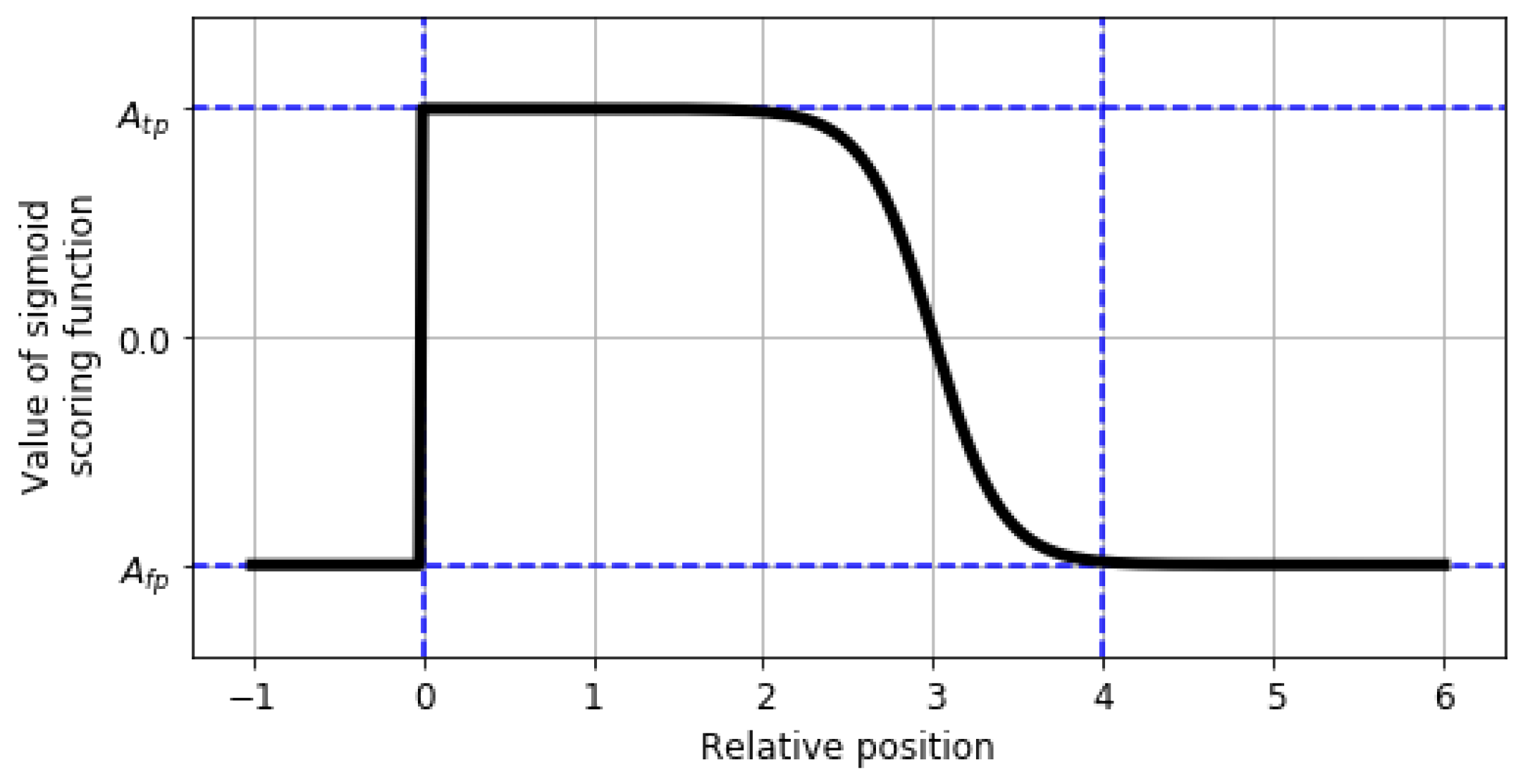
2.5. Performance Metric for Anomaly Detection Problem

Standard metrics, such as precision and recall, are not suitable for evaluating anomaly detection algorithms in systems where time series are used since they do not take into account the specifics of time. Because of this, some measurable characteristics of the algorithm performance, such as detection delay, are not accounted for either. For this reason, the Numenta Anomaly Benchmark performance scoring algorithm (or the NAB evaluating algorithm) was chosen from [9]. The purpose of this algorithm is to encourage early detection and to penalize false positives and false negatives.

The NAB evaluating algorithm contains three components, which must be tuned:

• the anomaly window;
• the application profiles;
• the scoring function.

The window in which the detected anomaly is perceived as a true positive is called an anomaly window (vertical blue lines in Figure 1). It is recommended by [9] to take a window equal to 10% of the sample length divided by the number of anomalies centered around a ground truth anomaly label. For technical systems, a more reasonable approach is to take the moment of occurrence of a hidden defect as a left boundary and the window width as the value characterizing the time taken to complete physical processes, during which the defect degrades.

In order to better understand the properties of each specific anomaly detection algorithm, the concept of an application profile was proposed. The application profile is a set of coefficients for true positives, false positives, and false negatives: $A_{TP},A_{FP},A_{FN}$, with $0\le A_{TP}$ and $-1\le A_{FP},A_{FN}\le 0$. Three application profiles are usually used: standard (standard weights of coefficients), reward low FPs (heavily penalizes FPs), and reward low FNs (heavily penalizes FNs). The application profiles (see

Table 1. Application profile for NAB scoring algorithm used in this work.

Metric	${\mathit{A}}_{\mathit{TP}}$	${\mathit{A}}_{\mathit{FP}}$	${\mathit{A}}_{\mathit{TN}}$	${\mathit{A}}_{\mathit{FN}}$
Standard	1.0	−0.11	1.0	−1.0
LowFP	1.0	−0.22	1.0	−1.0
LowFN	1.0	−0.11	1.0	−2.0

), given by [23], are used in our work.

The scoring function is used to weigh all true positives, false positives, and false negatives (true negatives are not used for evaluation, on principle), taking into account the coefficients and window width. Inside the window, only the first detection is used to weigh the true positives, while the rest are not taken into account. The sigmoidal scoring function gives high scores to early detections and gently penalizes detections outside of the window (see Figure 1). The equation of the scoring function is as follows:

$${\sigma }^A\left(y\right)=\left(A_{TP}-A_{FP}\right)\left(\frac{1}{1+e^{5y}}\right)-1$$

(9)

where y is the relative position of the detection within the anomaly window.

Score for each special time series d:

$$S_d^A=\left(\sum _{y\in Y_d}{\sigma }^A\left(y\right)\right)+A_{FN}{f}_d$$

(10)

where $Y_d$ is the set of data instances detected as anomalies by the detection algorithm and $f_d$ is the number of windows in which there are no detected anomalies.

To evaluate the anomaly detection algorithm in the entire set of D datasets, it is necessary to add them together:

$$S^A=\sum _{d\in D}{S}_d^A$$

(11)

The final score is:

$$S_{NAB}^A=100·\frac{S^A-S_{\mathrm{null}}^A}{S_{\mathrm{perfect}}^A-S_{\mathrm{null}}^A}$$

(12)

where $S_{\mathrm{perfect}}^A$ is a perfect score in which all anomalies are detected correctly and there are no false positives; $S_{\mathrm{null}}^A$ is a score in which no anomalies are detected.

The better the final score, the better the anomaly detection algorithm. The best result is equal to 100.

2.6. Python Library

One of the results of this work is the Anomaly Detection Library, named “ARIMAFD”. The library is implemented in the Python3 programming language. It includes an algorithm based on the ARIMA model for both forecasting and anomaly detection problems and others algorithms, as described in this paper. The advantages of algorithms from this library include the fact that a training set is not necessary, as well as the ability to work in online mode (batch processing). The disadvantages include the laborious process necessary to obtain the stationarity of the time series and to use heuristics.

The Anomaly Detection Library can be installed via the Python Package Index (PyPI) or via a link on GitHub https://github.com/waico/arimafd (accessed on 1 April 2021). For the purpose of unification, the commands and API design were developed in comparison with the scikit-learn library. An MIT License was used for the library.

3. Results

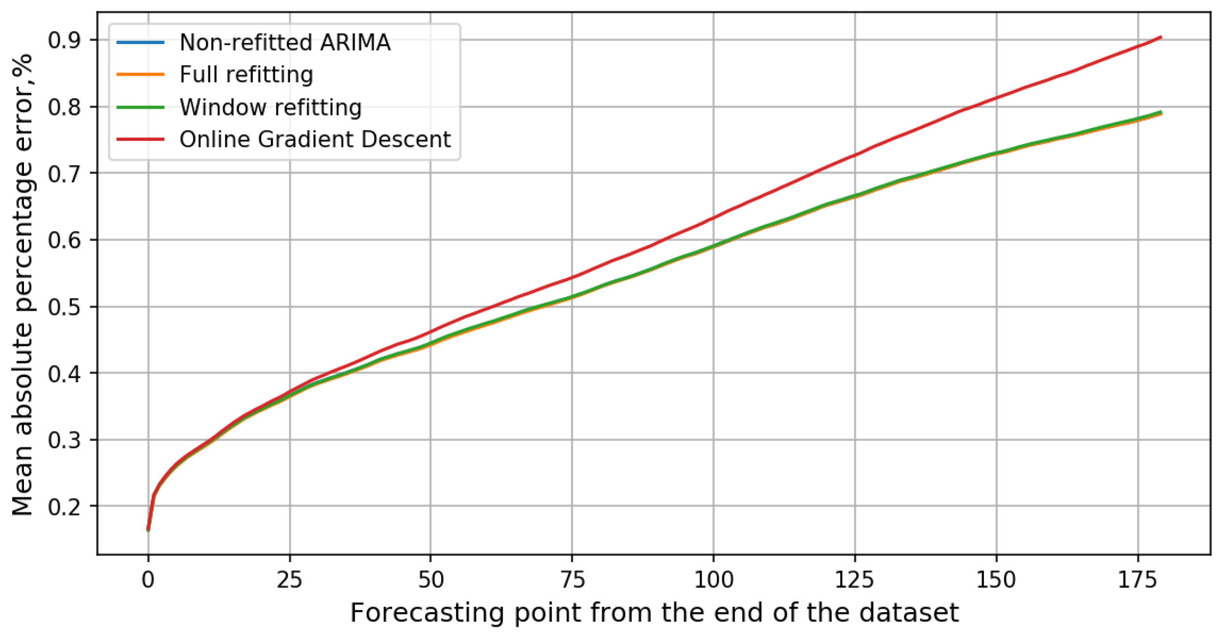
3.1. Forecasting by Online Algorithms

We used one specific time series, received from the sensors of the turbogenerator in a single operational mode without transients, which produces a total of 25 thousand samples in about half a month. The choice to use only one time series was due to our desire to compare the forecast results for one physical quantity. The time series was separated in the training and testing sets, accordingly, as 5 and 20 thousand samples (5 thousand samples are enough for the first training period). At each point in the testing set, the results were evaluated.

Table 2. Mean absolute percentage error of algorithms and ratio of learning time between algorithms. Non-refitted Autoregressive Integrated Moving Average (ARIMA) is an algorithm with unchanged weight coefficients for the testing set after fitting on the training set. The training time ratio is the ratio of the mean time taken for one model retraining procedure in the research algorithm compared to the mean time taken for one model retraining procedure in the Gradient Descent algorithm (0.09 s per one retraining procedure by the Intel Core i9-9900K processor).

Algorithm	MAPE, %				Training
	1 Point	30 Points	60 Points	180 Points	Time Ratio
Non-refitted ARIMA	0.1642	0.3828	0.4713	0.7886	0.00
Full refitting	0.1644	0.3808	0.4698	0.7887	205.24
Window refitting	0.165	0.3823	0.4725	0.7914	16.04
Online gradient descent	0.1667	0.3895	0.4936	0.9036	1.00

presents the results for time series forecasting by various online algorithms, as presented in Section 2.2. The results in Table 2 are presented in more detail in Figure 2. Despite the fact that the MAPE curves of the non-refitted ARIMA, full refitting and window refitting algorithms are visually merged into one (their similar numerical values are shown in Table 2), this picture shows the general behavior of the algorithms’ MAPE with an increase in the forecast horizon. We discuss the results more broadly in Section 4.

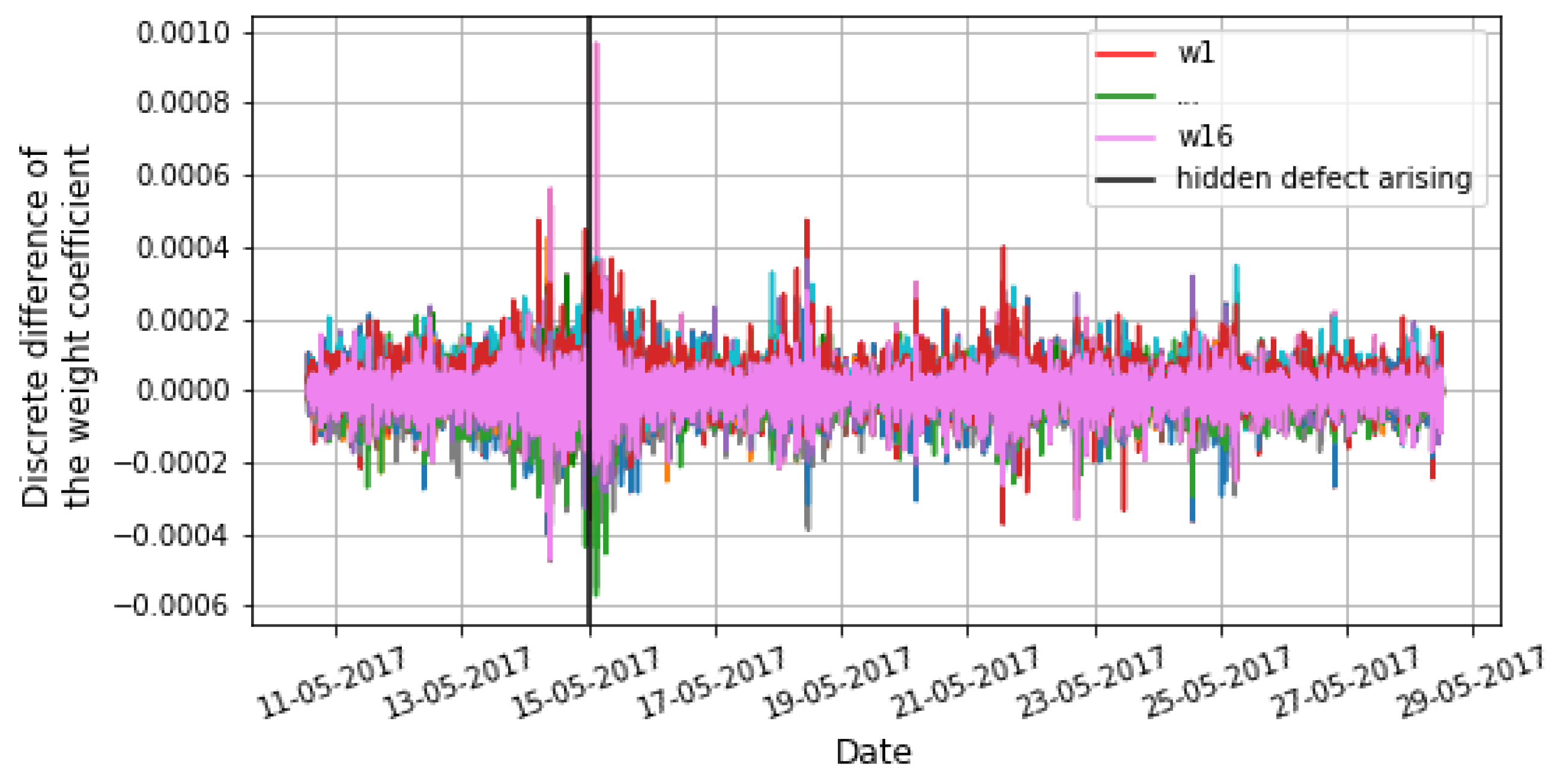
3.2. Anomaly Detection

Using the Numenta Anomaly benchmark [9], the developed anomaly detection algorithm based on the ARIMA model was tested.

Table 3. Score NAB from the scoreboard, where symbol * marks the result obtained by Algorithms 4 and 5.

Detector	Standard Profile	Reward Low FP	Reward Low FN
Perfect	100.0	100.0	100.0
Numenta HTM	70.5–69.7	62.6–61.7	75.2–74.2
CAD OSE	69.9	67.0	73.2
ARIMA AD algorithm with complex metric *	65.03	48.11	71.23
earthgecko Skyline	58.2	46.2	63.9
KNN CAD	58.0	43.4	64.8
One point prediction *	56.76	25.61	67.44
Relative Entropy	54.6	47.6	58.8
ARIMA AD algorithm with mean of max/std metric *	53.66	34.20	60.48
ARIMA AD algorithm with max of absolute value metric *	51.11	29.05	59.07
Random Cut Forest	51.7	38.4	59.7
Twitter ADVec v1.0.0	47.1	33.6	53.5
Windowed Gaussian	39.6	20.9	47.4
Etsy Skyline	35.7	27.1	44.5
ARIMA AD algorithm with Euclidean norm metric *	18.57	13.75	21.00
Bayesian Changepoint	17.7	3.2	32.2
EXPoSE	16.4	3.2	26.9
Random	11.0	1.2	19.5
Null	0.0	0.0	0.0

shows the scoreboard with the current state of the anomaly detection algorithm’s performance for the Numenta Anomaly benchmark, taken from the official page of the NAB on GitHub, and the results obtained using Algorithms 4 and 5. It can be seen from the table that the anomaly detection algorithm based on the ARIMA model shows strong results, and the algorithm based on Online Gradient descent and the complex metric took third place in accordance with this scoreboard.

This algorithm was also tested for its ability to detect hidden defects on real technical systems. Figure 3 shows the discrete differences in the weight coefficients of a turbogenerator-bearing vibration. From this figure, it can be seen that the received values increase in absolute value in a time moment in which, according to the commission, a defect arises, leading to the failure of the turbogenerator. Most of the other splashes are related to changes in the operation mode. For the case of the turbogenerator, one out of five hidden defects was detected.

4. Discussion

The results obtained during the forecasting experiment with various online algorithms were rather interesting and sometimes unexpected. The main results are shown in Table 2 and Figure 2. In actual fact, we expected to obtain results showing that non-refitted ARIMA had the worst result in terms of the MAPE, but this does not always happen when using real-world data. One of the possible reasons for this is that, halfway through a month, the technical system’s state does not change so much that the trained model becomes incorrect. On the other hand, the models have to be retrained sooner or later due to the turbogenerator’s continuous state changes and data drift. In this case, questions regarding the model retraining frequency and window selection for retraining are raised. The OGD algorithm allows us to dispel these questions since the model is updated constantly in real time. Additionally, the results clearly show that all algorithms are suitable for short-term forecasting. However, for long-term forecasting (180 points ahead), as expected [16], the OGD algorithm is less suitable, as the MAPE value is quite small (less than 1 percent) and still comparable with other algorithms’ results. The comparison of computational complexity also favors the OGD-based algorithm among the retrainable model-based algorithms (Table 2).

We also obtained interesting results for the anomaly detection problems at the turbogenerator. We detected one out of five hidden defects. At first glance, it seems that we obtained a weak result when applying this algorithm since just one hidden defect out of five was correctly detected. However, in actual fact, we were able to detect the emergence of an anomaly that has not been detected by existing diagnostic systems, and which ultimately led to serious financial losses. Moreover, this algorithm is an unsupervised change point detection algorithm, which means that it can contribute toward safety, even in the case of previously unknown hidden defects. As for the remaining four hidden defects, there is currently no understanding of whether they impacted the signals from the sensors and, consequently, the possibility of detection. Some more anomaly detection results were obtained using the Numenta Anomaly Benchmark. This benchmark was initially created to evaluate unsupervised real-time anomaly detection algorithms and includes time series data from various sources. The fact that the developed algorithm took third place on the corresponding scoreboard allows us to assert that the developed algorithm can be universally applied.

5. Conclusions

Many researchers are working on high-performance anomaly detection and forecasting algorithms with the ability to learn continuously and adapt to changing states. In this paper, we proposed a novel algorithm that can solve all of these challenging tasks simultaneously. It is based on the well-known ARIMA model, which is widely used for time-series modeling. The proposed algorithm works in online mode and uses unlabelled data, making it possible to solve tasks in an unsupervised manner. At the same time, it is much more computationally efficient and almost identically accurate when compared to classical ARIMA-based algorithms. All of these characteristics are essential for online process monitoring, including technical system diagnostics. A library in the Python3 programming language, using the “ARIMAFD” algorithm, was also proposed. As such, it is applicable both for anomaly detection and forecasting purposes.

For the forecasting problem, the proposed algorithm was compared with two pseudo-online algorithms and the non-learning ARIMA model. The results clearly show that all the algorithms turned out to be quite accurate, while their computational complexity and stability to changes in a system differed significantly, in favor of the developed online ARIMA-based algorithm. The strong ability of the proposed algorithm to find anomalies was confirmed by the fact that it took third place in the Numenta Anomaly Benchmark competition and the fact that it was able to detect a fault in the real-world data from the turbogenerator. The proposed algorithm not only beats the classical ARIMA-based 1-point-ahead prediction (Algorithm 5), but also outperforms most of the well-known online anomaly detection algorithms proposed by respectable researchers. While the results on the NAB prove the applicability of the proposed algorithm in various applications, successful anomaly detection in the turbogenerator data shows the clear benefits that the algorithm can bring in improving the safety and economic efficiency of power plants. Taken together, these results suggest that the combined algorithm we developed may be able to contribute to the development of technical diagnostics and online process monitoring.

The next steps in this direction should be the extension of a heuristics list that makes the overall algorithm more robust and invariant to the data, as well as the use of more advanced optimization algorithms.

References

1. Ahmad, S.; Purdy, S. Real-time anomaly detection for streaming analytics. arXiv 2016, arXiv:1607.02480. [Google Scholar]
2. Aminikhanghahi, S.; Cook, D.J. A survey of methods for time series change point detection. Knowl. Inf. Syst. 2017, 51, 339–367. [Google Scholar] [CrossRef] [PubMed] [Green Version]
3. Dobre, I.; Alexandru, A.A. Modelling unemployment rate using Box-Jenkins procedure. J. Appl. Quant. Methods 2008, 3, 156–166. [Google Scholar]
4. Rahman, M.; Islam, A.H.M.S.; Nadvi, S.Y.M.; Rahman, R.M. Comparative study of ANFIS and ARIMA model for weather forecasting in Dhaka. In Proceedings of the 2013 International Conference on Informatics, Electronics and Vision (ICIEV), Dhaka, Bangladesh, 17–18 May 2013. [Google Scholar] [CrossRef]
5. Asteriou, D.; Hall, S.G. Applied Econometrics; Macmillan International Higher Education: London, UK, 2015. [Google Scholar]
6. Box, G.E.; Jenkins, G.M.; Reinsel, G.C.; Ljung, G.M. Time Series Analysis: Forecasting and Control; John Wiley & Sons: Hoboken, NJ, USA, 2015. [Google Scholar]
7. Brockwell, P.J.; Davis, R.A.; Calder, M.V. Introduction to Time Series and Forecasting; Springer: New York, NY, USA, 2002; Volume 2. [Google Scholar]
8. Shumway, R.H.; Stoffer, D.S. Time Series Analysis and Its Applications: With R Examples; Springer: New York, NY, USA, 2017. [Google Scholar]
9. Lavin, A.; Ahmad, S. Evaluating Real-Time Anomaly Detection Algorithms—The Numenta Anomaly Benchmark. In Proceedings of the 2015 IEEE 14th International Conference on Machine Learning and Applications (ICMLA), Miami, FL, USA, 9–11 December 2015. [Google Scholar] [CrossRef] [Green Version]
10. Schmidt, F.; Suri-Payer, F.; Gulenko, A.; Wallschlager, M.; Acker, A.; Kao, O. Unsupervised Anomaly Event Detection for Cloud Monitoring Using Online Arima. In Proceedings of the 2018 IEEE/ACM International Conference on Utility and Cloud Computing Companion (UCC Companion), Zurich, Switzerland, 17–20 December 2018. [Google Scholar] [CrossRef]
11. Zinkevich, M. Online convex programming and generalized infinitesimal gradient ascent. In Proceedings of the 20th International Conference on Machine Learning (ICML-03), Washington, DC, USA, 21–24 August 2003; pp. 928–936. [Google Scholar]
12. Anava, O.; Hazan, E.; Mannor, S.; Shamir, O. Online Learning for Time Series Prediction. arXiv 2013, arXiv:1302.6927v1. [Google Scholar]
13. Chen, Q.; Guan, T.; Yun, L.; Li, R.; Recknagel, F. Online forecasting chlorophyll a concentrations by an auto-regressive integrated moving average model: Feasibilities and potentials. Harmful Algae 2015, 43, 58–65. [Google Scholar] [CrossRef]
14. Leithon, J.; Lim, T.J.; Sun, S. Renewable energy management in cellular networks: An online strategy based on ARIMA forecasting and a Markov chain model. In Proceedings of the 2016 IEEE Wireless Communications and Networking Conference, Doha, Qatar, 3–6 April 2016. [Google Scholar] [CrossRef]
15. Yao, L.; Su, L.; Li, Q.; Li, Y.; Ma, F.; Gao, J.; Zhang, A. Online Truth Discovery on Time Series Data. In Proceedings of the 2018 SIAM International Conference on Data Mining; Society for Industrial and Applied Mathematics: Philadelphia, PA, USA, 2018; pp. 162–170. [Google Scholar] [CrossRef] [Green Version]
16. Anava, O.; Hazan, E.; Zeevi, A. Online time series prediction with missing data. In Proceedings of the International Conference on Machine Learning, Lille, France, 6–11 July 2015; pp. 2191–2199. [Google Scholar]
17. Giraud, C.; Roueff, F.; Sanchez-Perez, A. Aggregation of predictors for nonstationary sub-linear processes and online adaptive forecasting of time varying autoregressive processes. Ann. Stat. 2015, 43, 2412–2450. [Google Scholar] [CrossRef]
18. Enqvist, P. A convex optimization approach to n, m (ARMA) model design from covariance and cepstral data. SIAM J. Control Optim. 2004, 43, 1011–1036. [Google Scholar] [CrossRef]
19. Vasiliev, F. Optimization Methods. Second Book; Factorial Press: Moscow, Russia, 2017. [Google Scholar]
20. USSR State Committee for Product Quality and Standards Management; Ministry of Automotive and Agricultural Engineering of the USSR; USSR Academy of Sciences; Ministry of Higher and Secondary Education of the RSFSR; State Commission of the Council of Ministers of the USSR for food purchases. Technical Diagnostics. Terms and Definitions. GOST 20911-89; Interstate Standard: Moscow, Russia, 1991. [Google Scholar]
21. Yaacob, A.H.; Tan, I.K.; Chien, S.F.; Tan, H.K. ARIMA Based Network Anomaly Detection. In Proceedings of the 2010 Second International Conference on Communication Software and Networks, Bangalore, India, 5–9 January 2010. [Google Scholar] [CrossRef]
22. Krishnamurthy, B.; Sen, S.; Zhang, Y.; Chen, Y. Sketch-based change detection: Methods, evaluation, and applications. In Proceedings of the 3rd ACM SIGCOMM Conference on Internet Measurement, Miami Beach, FL, USA, 27–29 October 2003; pp. 234–247. [Google Scholar]
23. Ishimtsev, V.; Nazarov, I.; Bernstein, A.; Burnaev, E. Conformal k-NN Anomaly Detector for Univariate Data Streams. arXiv 2017, arXiv:1706.03412v1. [Google Scholar]
Figure 1. Scaled sigmoid function.
Applsci 11 03194 g001
Figure 2. Absolute forecasting error averaged over all refitting. Forecasting horizon is 180 points.
Applsci 11 03194 g002
Figure 3. The discrete difference in the modernized ARIMA weight coefficients for turbogenerator-bearing vibration time series. The black vertical line shows the time moment in which the hidden defect arose.
Applsci 11 03194 g003