Article

Uncertainty of the 2D Resistivity Survey on the Subsurface Cavities

by
Yonatan Garkebo Doyoro
1,2,
Ping-Yu Chang
2,3,* and
Jordi Mahardika Puntu
2
1
Earth System Science, Taiwan International Graduate Program (TIGP), Academia Sinica, Taipei 115, Taiwan
2
Department of Earth Science, National Central University, Taoyuan 320, Taiwan
3
Earthquake-Disaster, Risk Evaluation and Management Centre, National Central University, Taoyuan 320, Taiwan
*
Author to whom correspondence should be addressed.
Appl. Sci. 2021, 11(7), 3143; https://doi.org/10.3390/app11073143
Submission received: 23 February 2021 / Revised: 22 March 2021 / Accepted: 29 March 2021 / Published: 1 April 2021
(This article belongs to the Special Issue Advances in Applied Geophysics)

Abstract

:
We examined the uncertainty of the two-dimensional (2D) resistivity method using conceptual cavity models. The experimental cavity study was conducted to validate numerical model results. Spatial resolution and sensitivity to resistivity perturbations were also assessed using checkerboard tests. Conceptual models were simulated to generate synthetic resistivity data for dipole-dipole (DD), pole-dipole (PD), Wenner–Schlumberger (WS), and pole-pole (PP) arrays. The synthetically measured resistivity data were inverted to obtain the geoelectric models. The highest anomaly effect (1.46) and variance (24,400 Ω·m) in resistivity data were recovered by the DD array, whereas the PP array obtained the lowest anomaly effect (0.60) and variance (2401 Ω·m) for the shallowest target cavity set at 2.2 m depth. The anomaly effect and variance showed direct dependency on the quality of the inverted models. The DD array provided the highest model resolution that shows relatively distinct anomaly geometries. In contrast, the PD and WS arrays recovered good resolutions, but it is challenging to determine the correct anomaly geometries with them. The PP array reproduced the lowest resolution with less precise anomaly geometries. Moreover, all the tested arrays showed high sensitivity to the resistivity contrasts at shallow depth. The DD and WS arrays displayed the higher sensitivity to the resistivity perturbations compared to the PD and PP arrays. The inverted models showed a reduction in sensitivity, model resolution, and accuracy at deeper depths, creating ambiguity in resistivity model interpretations. Despite these uncertainties, our modeling specified that two-dimensional resistivity imaging is a potential technique to study subsurface cavities. We inferred that the DD array is the most appropriate for cavity surveys. The PD and WS arrays are adequate, while the PP array is the least suitable for cavity studies.

1. Introduction

Resistivity imaging is a geophysical method, which has become a powerful tool to investigate shallow subsurface features. The technique has been widely used in several fields of geosciences, such as structural geological [1,2,3,4,5], hydrogeological [6,7], geohazard [8,9], and environmental [10,11,12,13] studies. Subsurface cavity structures most commonly occur in carbonate terrain through the dissolution of carbonate rocks. Isostatic subsidence of the developed cavity can impose substantial damage on structural, environmental, and human values. Engineering structures require subsurface investigation to map and assess the presence of cavities, which reduces construction risks. Several geophysical methods are applied in order to determine the size, position, and depth of the subsurface cavities. Among the geophysical methods, resistivity imaging is a commonly used technique to identify cavity structures [12,14,15,16].
Despite the applicability success, resistivity imaging often leads to non-unique models of the subsurface. It is well-known that the resistivity method produces uncertainties in final model interpretation because of the inherited ambiguity in data inversion. This is because the inversion of electrical resistivity data is a non-linear problem, while the solutions are obtained using a linearized forward model [17,18,19]. The resistivity survey measures a limited number of data points at a discrete electrode spacing, which also constrained to obtain a unique resistivity response of the subsurface structures [20]. Thus, the delineation and mapping of subsurface cavities remain challenging in environmental studies using resistivity imaging [11,21].
Different factors can be considered in cavity studies, such as target size, depth, orientation, geometry, filling materials, and resistivity contrast with the host medium. The measured apparent resistivity data gives an average value representing a volume of geological material. The volume-averaging property of the resistivity method may obscure the small-scale cavity. The sparse sampling and less sensitivity characteristics of the resistivity method with increased survey depth may also obscure cavity information [15,22]. These factors may delimit the technique and the type of array to be used in resistivity imaging [23,24]. Even though the cavity depth is small and situated at a relatively deeper depth, substantial resistivity contrast between the cavity and the host medium can reveal suitable imaging results [12,21,25].
Moreover, selecting the best electrode configuration to recover the material variations over a cavity zone is the main problem in resistivity study. Among the commonly used electrode configurations, the dipole-dipole (DD) array is widely used to detect subsurface lateral changes, yet it is more vulnerable to measurement noises and often produces a low signal-to-noise ratio. The pole-dipole (PD) configuration has relatively higher signal strength compared to the DD array. However, the PD array provides asymmetrical resistivity data that adds bias to the inverted models [21,25], whereas the Wenner–Schlumberger (WS) configuration is moderately sensitive to both lateral and vertical variations. The WS array also has a higher signal-to-noise ratio, yet it recovers a relatively lower resistivity contrast compared to the DD arrays [26,27]. On the other hand, the pole-pole (PP) array can produce comprehensive horizontal data coverage and survey greater depths as compared to other types of arrays. However, its remote electrode is highly sensitive to ambient (telluric) noises [21,25]. Therefore, each array has its advantages and limits in relation to cavity imaging, and a comprehensive study is needed to ascertain which configuration is the most suitable one.
Many studies have been carried out to compare the pros and cons of the most commonly used resistivity imaging arrays. The study in Reference [22] stressed on the measurement sensitivities of the arrays to compare the Wenner, dipole-dipole, pole-dipole, pole-pole, Wenner–Schlumberger, and gradient arrays. The dipole-dipole, pole-dipole, and pole-pole arrays were compared based on the depth of investigation [28]. Another study [25] performed numerical simulation for five synthetic models using different arrays: pole-pole, pole-dipole, half-Wenner, Wenner, Schlumberger, dipole-dipole, Wenner-β, γ-array, moving gradient, and midpoint-potential-referred measurement arrays. They suggested the moving gradient array, pole-dipole, dipole-dipole, and Schlumberger arrays. However, the final choice of the arrays should be decided based on the type of expected geology as the subsurface geological distributions have a significant impact on the arrays’ imaging ability. Various numerical simulations for different noise perturbations were conducted by emphasizing the data-acquiring ability of the arrays: Wenner, dipole-dipole, Wenner–Schlumberger, and linear grid [29]. Comparison of arrays (Wenner, Wenner–Schlumberger, dipole-dipole, pole-dipole, and pole-pole) for imaging buried tunnels showed better results using the Wenner–Schlumberger and dipole-dipole arrays [30]. The Wenner-Alph and Wenner–Schlumberger showed a better result than the dipole-dipole array for reconstructing the landslide model [31]. Among the Wenner, dipole-dipole, pole-dipole, and pole-pole arrays used for detecting the cleared-wall foundations, the Wenner and dipole-dipole arrays were selected as the best methods [32]. From the numerical modeling using the dipole-dipole, pole-dipole, dipole-pole, and pole-pole arrays, the pole-dipole array showed the best result for modeling sinkhole [33]. The dipole-dipole array imaged the sinkhole better than the Wenner and Schlumerger arrays [21]; in contrast, the Wenner array showed better model resolution than the dipole-dipole array for surveying the underground three-dimensional cavity [34]. Even though these studies have evaluated the effectiveness of resistivity imaging for different geological conditions, there are no studies that assess the constraints of resistivity imaging as well as the configuration best-suited for imaging subsurface cavities.
In this study, we present the resistivity imaging uncertainties using synthetic and experimental cavity models. We simulated a cavity model with different depths, sizes, orientations, geometries, and filling materials, as these features substantially change the model result of the resistivity imaging [25]. Additionally, arrays’ spatial resolution and sensitivity were examined. The modeling was performed for the DD, PD, WS, and PP arrays since the resolution of data inversion is also constrained by the type of arrays. A model with cells of a given resistivity value was constructed, and the apparent resistivity data were formulated using the finite-element method. Inversion of measured resistivity data was provided with the two-dimensional (2D) geoelectric models. We examined the constraints of the resistivity method on recovering cavity information for different cavity models. Moreover, the potential capability of arrays that can reveal the cavity structures was tested and identified.

2. Methodology

Resistivity imaging is usually applied in unknown geologic conditions, which cannot fully recover the true subsurface structure for the measured data [35]. Using a synthetic model under the controlled circumstance is a fundamental approach to assessing imaging method accuracy. A synthetic modeling so-called forward-inverse cycle consists of standard geophysical inversion processes, which inverts the synthetically measured data by the mathematical method to get specific resistivity distribution. It also implements a forward calculation that predicts a set of resistivity data based on a given synthetic model [36]. We used forward-inverse modeling to examine resistivity imaging uncertainties and identify appropriate arrays for cavity probing based on model accuracy, resolution, and sensitivity. In the following section, we systematically present modeling procedures and data analysis.

2.1. Forward-Inverse Modeling

We developed resistivity conceptual models to represent karstic subsurface structures in limestone terrain. In nature, cavities have different depth of burial, size, geometry, and orientation that can be air-filled, water-filled, or sediment-filled [37,38]. To study the effect of these cavity properties on the recovering ability of the 2D resistivity methods (DD, PD, WS, and PP arrays), we generate different synthetic models. The cavity depths, sizes, orientations, and geometries were considered in our numerical modeling. Since the survey depth has a significant effect on the resistivity model resolution, we focused on the arrays’ performance with cavity depths. We set an air-filled cavity model at six different depths, naming cavity targets as T1, T2, T3, T4, T5, and T6, with the depths of 2.2, 4.2, 6.2, 8.2, 10.2, and 12.2 m, respectively (as shown in Figure 1). The target cavity T2 was used for further analysis as its depth is more common in cavernous limestone terrain. We numerically modelled the conductive cavities by using a filling of dry and saturated clay; however, the resistivity of the cavity filling material is a function of the particle size, saturation, and resistivity of the pore fluid [39].
As this study specifically examines the case of cavities in karstic terrain, the conceptual models’ host medium was considered as uniform dry limestone rock with a resistivity value of 1000 Ω·m. Only in the case of conductive cavity modeling, when the water table is above the cavity, did we use a resistivity value of 450 Ω·m for the host limestone [38,40]. We used the resistivity value of 10,000 Ω·m for the air-filled cavity [11], 90 Ω·m for the cavity filled with dry clay [41], and 50 Ω·m for the cavity filled with saturated clay [33]. The arrays such as DD, PD, WS, and PP were used for surface probing, which apply 89 electrodes with 1 m spacing.
Furthermore, the synthetic reconstruction test, known as the checkerboard resolution test, was implemented in this study. The checkerboard test is often applied in seismic studies to examine the lateral resolution of the tomographic image. The alternating pattern of positive and negative anomalies along a spatial dimension is used to develop the checkerboard model. Inversion was performed for synthetically measured data to evaluate the recovered model resolution [42,43,44].
We applied the checkerboard resolution test to assess the resolution of resistivity tomogram in-depth cross-section along the survey profiles. Three different size scenarios of checkerboard cells were used to examine the anomaly size effect on the spatial resolution of the recovered models. We used a checkerboard cell size with 1 (vertical) × 2 m (horizontal) dimensions in scenario 1. In scenario 2, the size increased by the factor of two, i.e., 2 × 4 m cell size, while the factor of four was used in scenario 3, i.e., 4 × 8 m cell size. The background resistivity (1000 Ω·m) was perturbed by ±20% resistivity anomaly; thus, the checkerboard cells were assigned by alternating resistivity values of 800 and 1200 Ω·m.
Sensitivity in resistivity study can be used in different ways [22,45,46,47,48]. In this study, sensitivity was used to assess how the arrays are sensitive to different resistivity perturbations (contrasts). In addition to evaluating the spatial resolution of the inverted tomogram, we applied the checkerboard test to examine the sensitivities of the array (DD, PD, WS, and PP). We used a checkerboard cell size of 2 m in the vertical direction and 4 m in the horizontal direction with background resistivity of 1000 Ω·m, which was perturbed by ±20%, 40%, 60%, and 80% anomalies.
The conceptual models were simulated to generate synthetic resistivity data. We implemented the AGI EarthImagerTM 2D software [49] for the model simulations. The finite-element modeling calculates the resistivity data using a partial differential equation [50]. Throughout the entire lateral and vertical mesh formulations, 1.0 m thickness and depth increment factor were used. Finer meshes of 0.5 × 0.5 m were applied to increase the forward modeling accuracy. The simulation was perturbed using Gaussian noise (a random value generated with zero mean and 3% standard deviation) in order to integrate the field data-acquisition noise effects.
We applied a robust inversion scheme to recover the 2D geoelectric model. It optimizes [51] the least-square method [52] by integrating the weighting matrices, giving approximately equal weight for data misfit and model roughness vector in the inversion processes. Robust inversion also provides improved inversion results for sharper resistivity models. It obtains more compacted anomalies, and it is a sound method to reduce data outliers [53]. Consistently, in our modeling, the robust inversion provided minor inversion artefacts, especially for large resistivity contrasts over a short profile distance.
The use of a larger grid size makes the inversion process more efficient; however, it leads to low model resolutions. Further discretization of the model parameters, on the contrary, does not show substantial changes in the model structure rather than smoothening the transition zones [53]. Hence, we applied an optimal grid of 1 × 1 m for the inversion of apparent resistivity data. The damping and smoothing factors were set to 10 initially, and these factors were reduced iteratively.

2.2. Data Analysis

We analyzed the numerically measured apparent resistivity data using a statistical variance, which describes how far the data are spread out from the average value. Variance was also used to examine the association of measured resistivity data with the cavities since the resistivity method explicitly depends on the subsurface resistivity variations. A higher variance may indicate larger resistivity contrast and vice versa. Hence, the variance (σρ) for the measured apparent resistivities (ρi) with the mean value (µρ) was calculated as follows:
σ ρ 2 =   1 N   i = 1 N ( ρ i µ ρ ) 2
The anomaly effect (AE) was first introduced by Militzer [54], commonly used to evaluate arrays’ measuring abilities. The anomaly effect was also used to examine arrays’ applicability for different subsurface features, and it is calculated using the expression [25,55]:
AE = | max ( ρ a ρ av ) min ( ρ a ρ av ) |
where ρ max , ρ min , and ρ av represent the maximum, minimum, and average apparent resistivities, respectively. We applied the anomaly effect to assess the recovering abilities of the arrays and inspect the corresponding image quality as a function of cavity depth.
Data misfit between the measured and predicted apparent resistivity using relative root mean square (RMS) error [56] was used to assess arrays’ inversion error with cavity depth.
The depth of investigation (DOI) index [28,57] calculated the depth below, for which the obtained model influenced by the reference model rather than the measured data, by inverting the same dataset twice with different reference models (m01 and m02) using 0.1 and 10 times of the average apparent resistivity. DOI value of the bottom model (Rb) was used to normalize the DOI index, and it is presented as:
DOI   ( x , z ) =   m 1 ( x , z )   m 2   ( x , z ) R b ( m 01 m 02 )
where m1 and m2 indicate the inverted resistivity values of the same cell for the two inversions.
We also examined the arrays’ model accuracy based on the image correlation between the actual and inverted cavity models. The similarities were quantified using a statistical correlation coefficient that is expressed by:
Correl   ( ρ i , ρ a ) = ( ρ i µ i ) ( ρ a µ a ) ( ρ i µ i ) 2 ( ρ a µ a ) 2
where ρi is the inverted resistivity data points, ρa is the actual model resistivity data points, µi is the mean value for the inverted resistivity data, and µa is the mean value for the actual resistivity data.

3. Results and Discussion

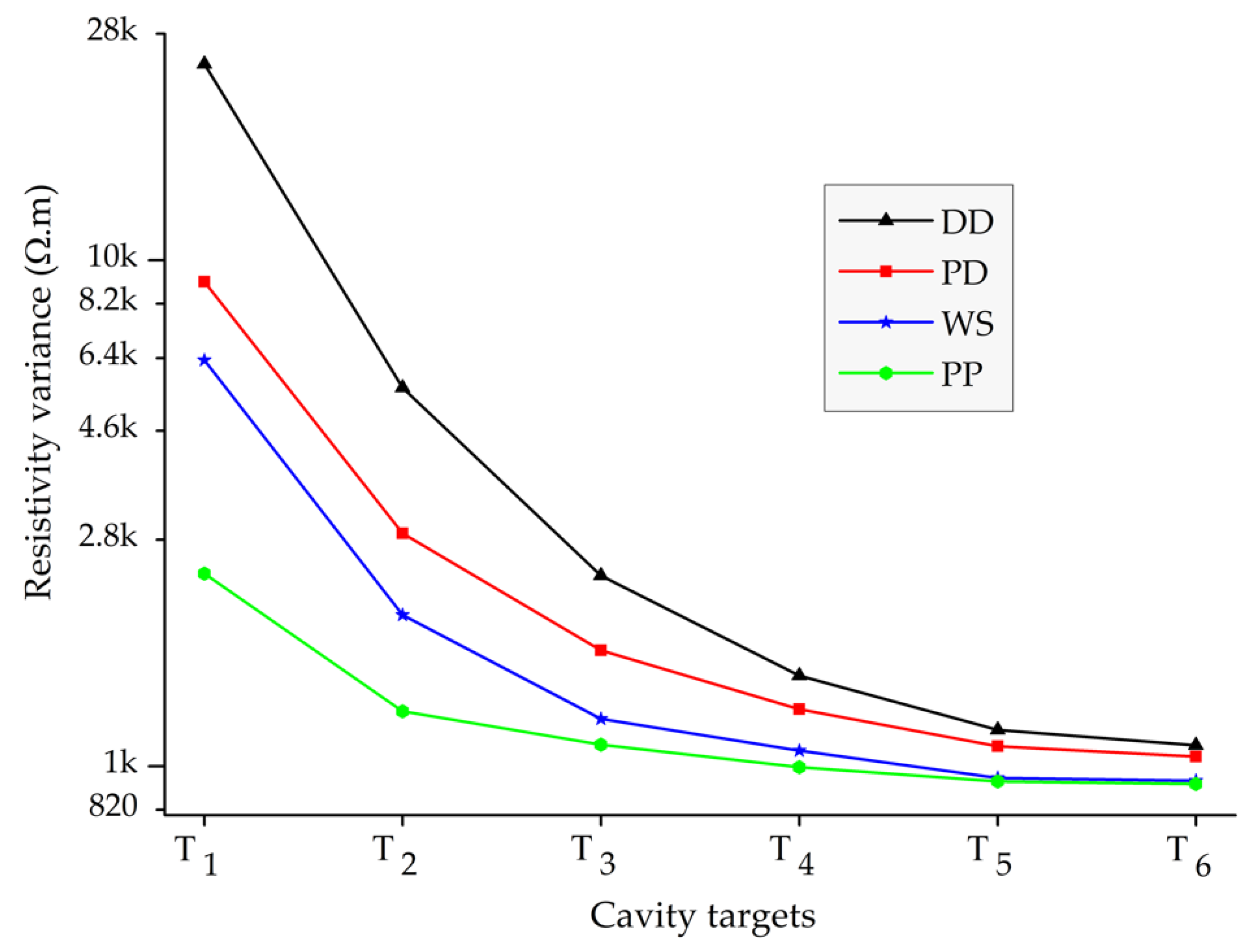
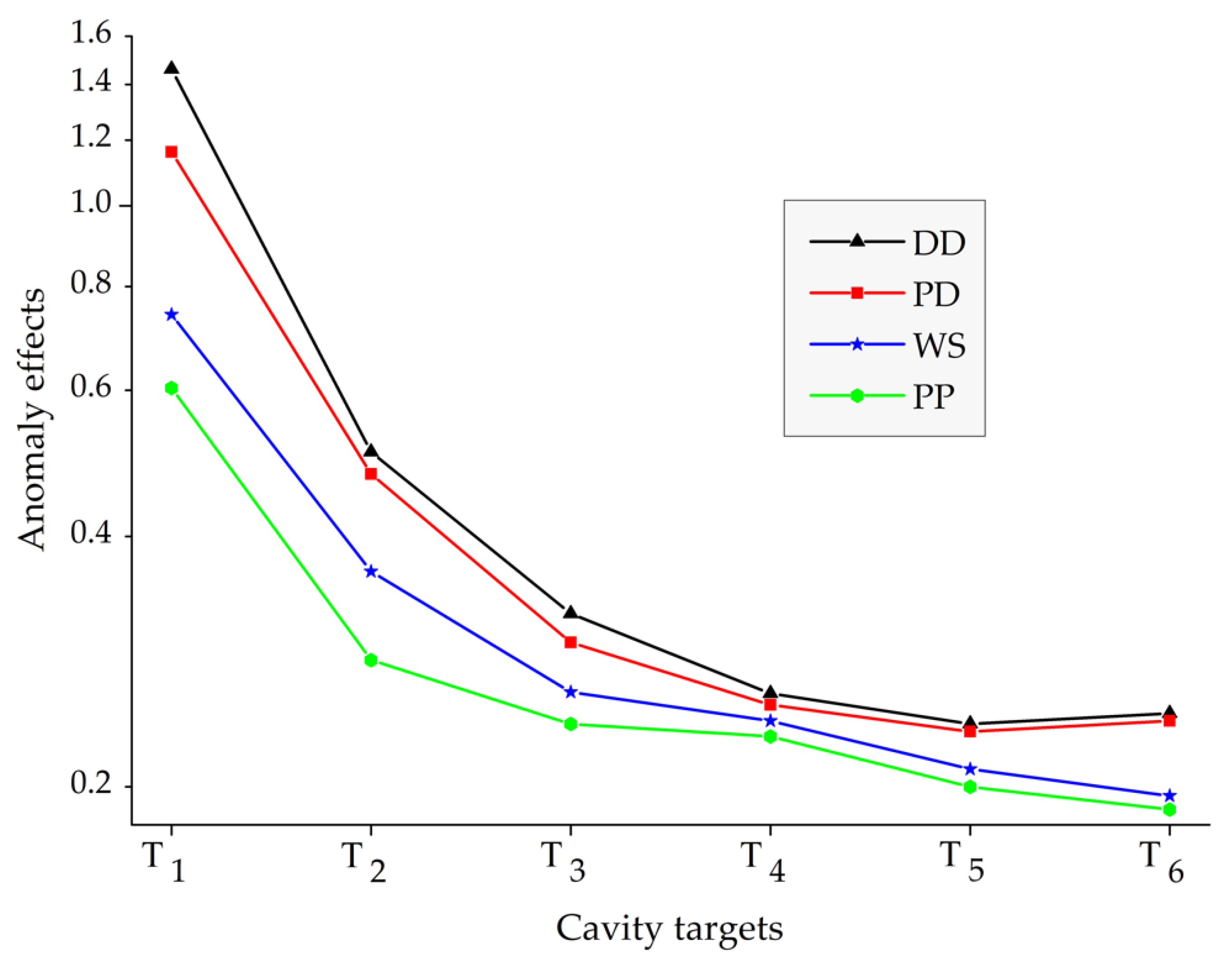
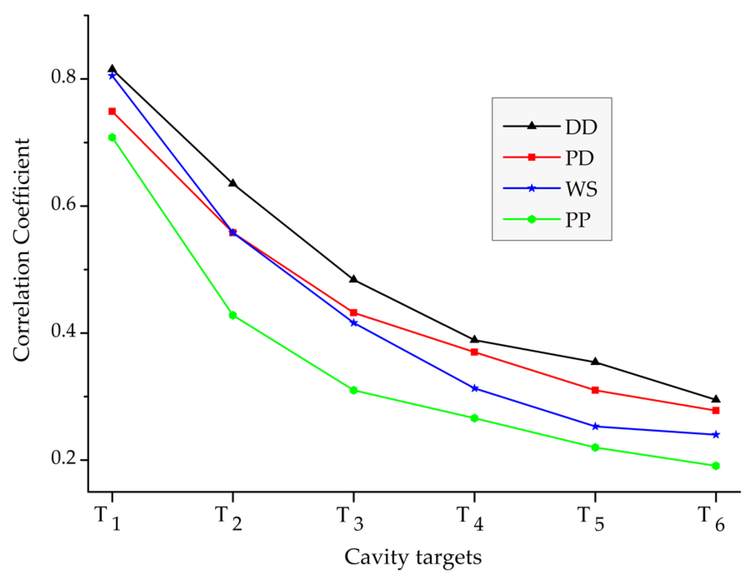
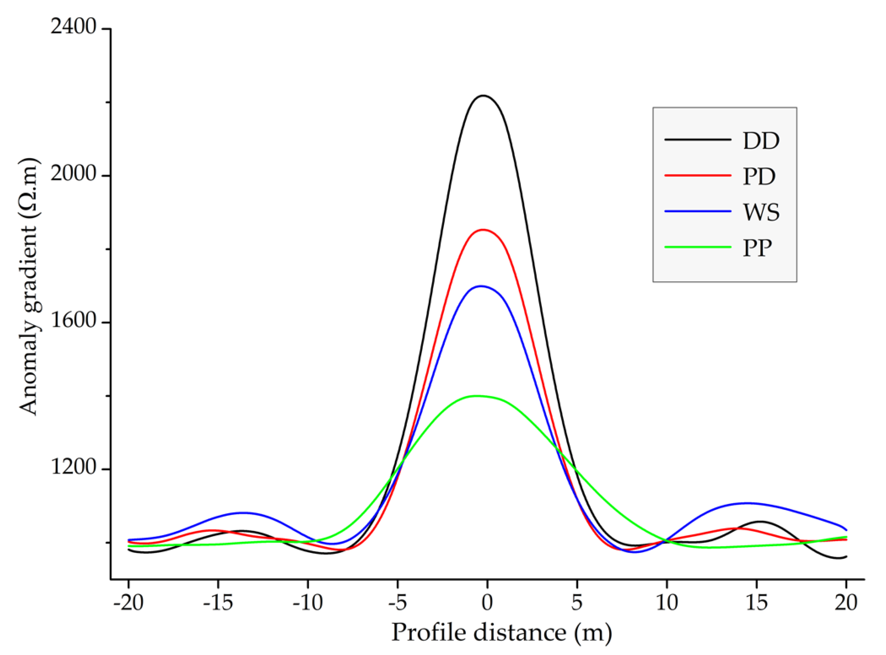
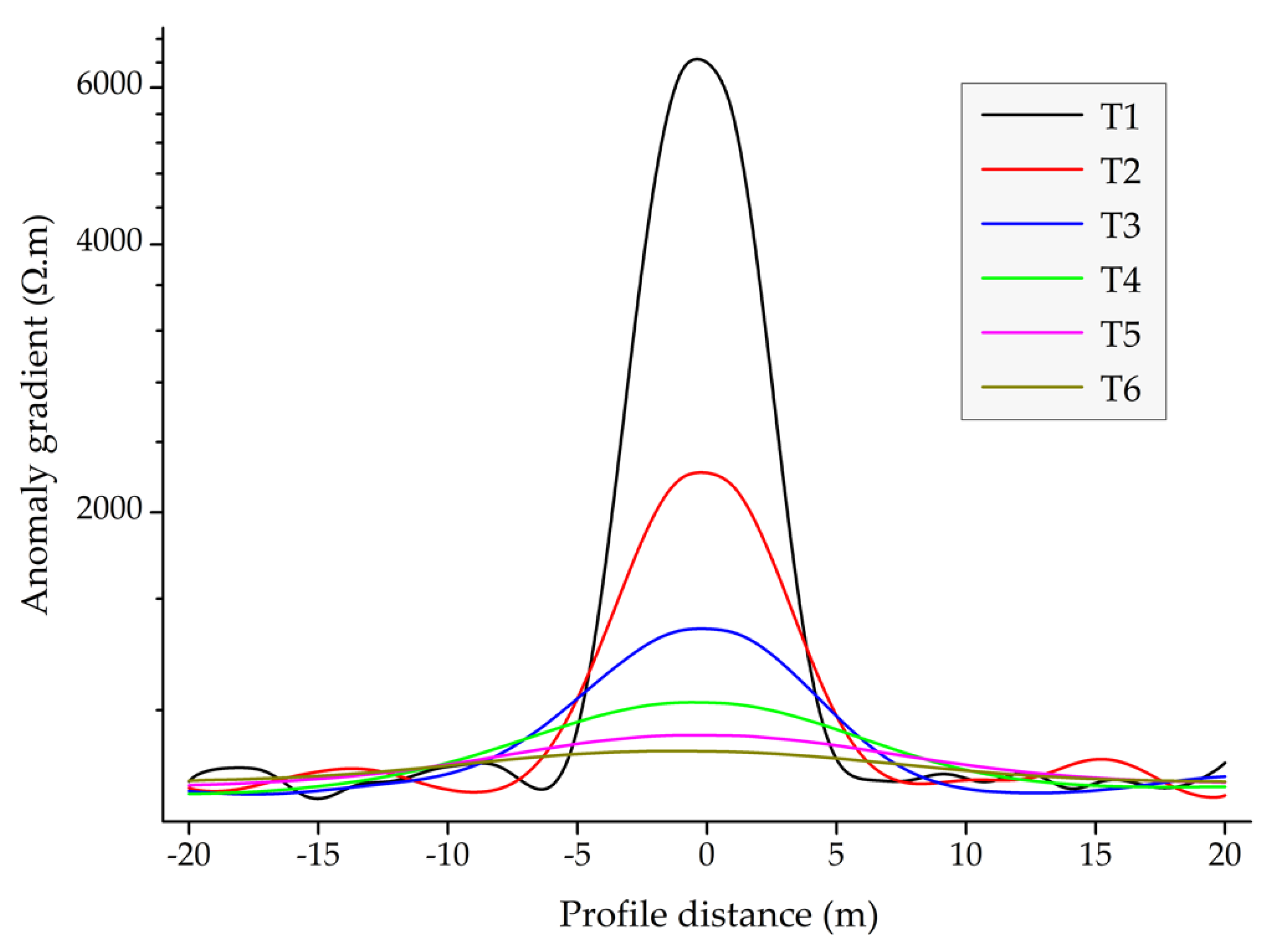
3.1. Array Detection Ability

The data recovering ability of different arrays may vary when applied to a specific subsurface structure [47]. In this study, we used the statistical variance to examine the measuring ability of arrays with regard to cavity depth. As depicted in Figure 2, when modeling the target cavity T1 (at 2.2 m depth), resistivity data exhibited the variances of 24,400, 9058, 6341, and 2401 Ω·m for the DD, PD, WS, and PP arrays, respectively. In contrast, for the target cavity T6 (at 12.2 m depth), resistivity data showed a statistical variance of 1100, 1044, 936, and 900 Ω·m for the DD, PD, WS, and PP arrays, respectively. The DD array depicted the maximum variance in resistivity data, whereas the PD and WS arrays produced moderate variances. The resistivity data from the PP array indicated the least variance. The results also show a linear dependence between the variance of the resistivity data and the accuracy of the cavity model recovered. Figure 2 shows that the decrease in resistivity data variance with increasing cavity depth is likely due to decreasing measurement sensitivity with survey depth [22].
To obtain reliable and high-resolution resistivity tomograms, the arrays used in the measurements should provide data with maximum anomaly information [47]. Thus, we calculated the anomaly effect of the numerically measured resistivity data, which shows the recovering ability of the arrays for different air-filled cavity depths. As shown in Figure 3, the highest anomaly effects of 1.46, 1.16, 0.74, and 0.6 for the corresponding arrays of DD, PD, WS, and PP were shown for the simulation of the shallowest cavity T1. In contrast, the arrays DD, PD, WS, and PP exhibited the lowest anomaly effects of 0.245, 0.24, 0.19, and 0.18 respectively, for the deepest cavity T6. The dielectric nature of the cavity causes the arrays to acquire resistivity data with higher anomaly effects, mainly for the shallow cavity depth [11]. The DD array provided maximum anomaly effect, while the PP array exhibited minimum anomaly effect, similar to other studies [55]. In comparison, the PD and WS arrays depicted moderate anomaly effects. The anomaly effect shows a linear relationship with the measurement sensitivity of the array [47]. This could be the reason behind the decline of anomaly effects with an increasing cavity depth (Figure 3). The higher sensitivity near the electrode location may enable the arrays to get a more pronounced anomaly effect. On the other hand, the low sensitive zone of the far electrode position might limit the arrays to recover the higher anomaly effect.

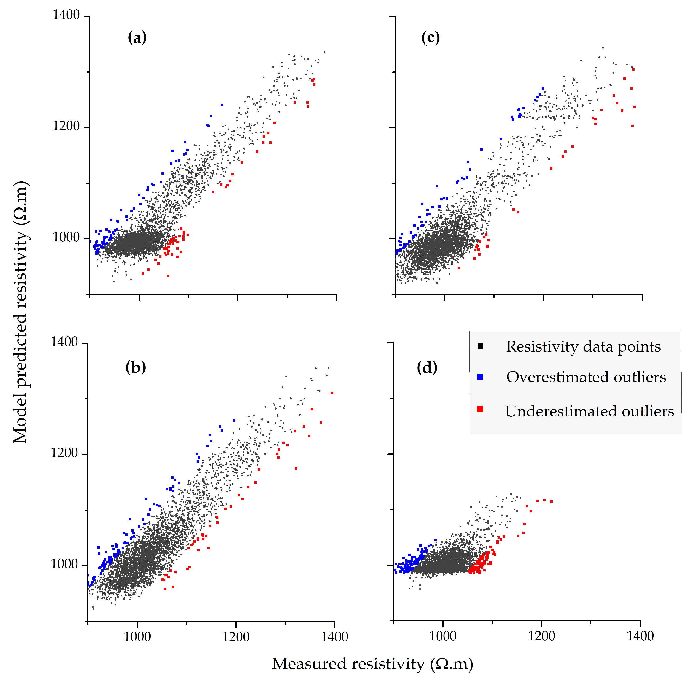
3.2. Inversion Error

The presence of noisy data points can create a large discrepancy between the inverted and the resistivity model, producing artefacts in the inverted resistivity models [58]. In this study, we used the statistical 95% confidence interval to identify those noisy data points. Figure 4 exhibits the model predicted versus synthetically measured apparent resistivity datasets for the target cavity T2. About 5% of the data points situated on the upper and lower limit of the scatter plots were specified as outliers. The predicted resistivity was significantly overestimated for smaller values of measured resistivity data points that may be related to the background medium (host limestone unit). On the other hand, the predicted resistivity was considerably underestimated for the extreme values of measured resistivity, probably due to the smoothing of the resistivity contrast between the background medium and the cavity by the inversion method [59].
The inversion model with a smaller error usually provides a more accurate image; however, it does not necessarily mean that an inverted model with a smaller RMS error can give a realistic final model. This is because the inversion algorithm will sometimes tend to overfit the measured data for a larger number of iterations. For large resistivity contrasts, the inversion algorithm can progressively increase the inverted resistivity value from one iteration to the next without a considerable change in RMS error [60]. Consequently, a best-inverted model is often attained at a relatively low iteration number [61]. In cavity modeling, we used the model outputs with a maximum number of 4 iterations to reduce data overfit as further iterations did not improve the results. The result also depicted a considerable RMS error for inversion of high-contrast resistivity data. It is well-known that the surface resistivity method can acquire high-contrast resistivity data for shallower structures (e.g., cavity) than the deeper ones. As a result, the inversion of shallower cavity models exhibited higher RMS error than the deeper models (Figure 5), yet the inversion processes were stopped as long as the absolute data misfit value closes perturbation noise level (3%). Resistivity modeling may also reveal high model resolution, although the inversion provides large RMS error and vice versa. For example, the DD array showed a higher model resolution than the PP array; however, the DD array produced a larger RMS error than the PP array (Figure 5).

3.3. Model Accuracy, Resolution, and Sensitivity

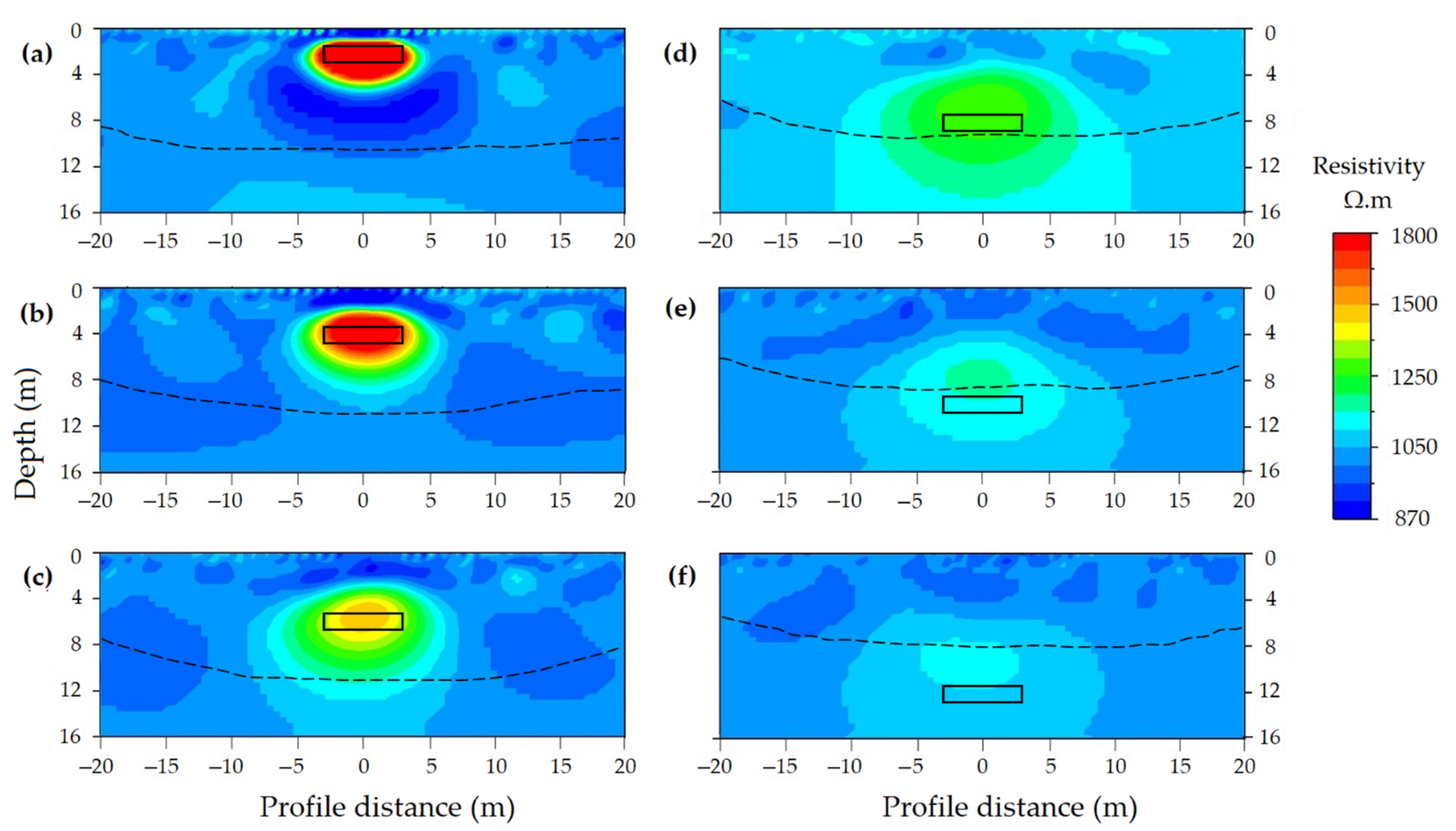
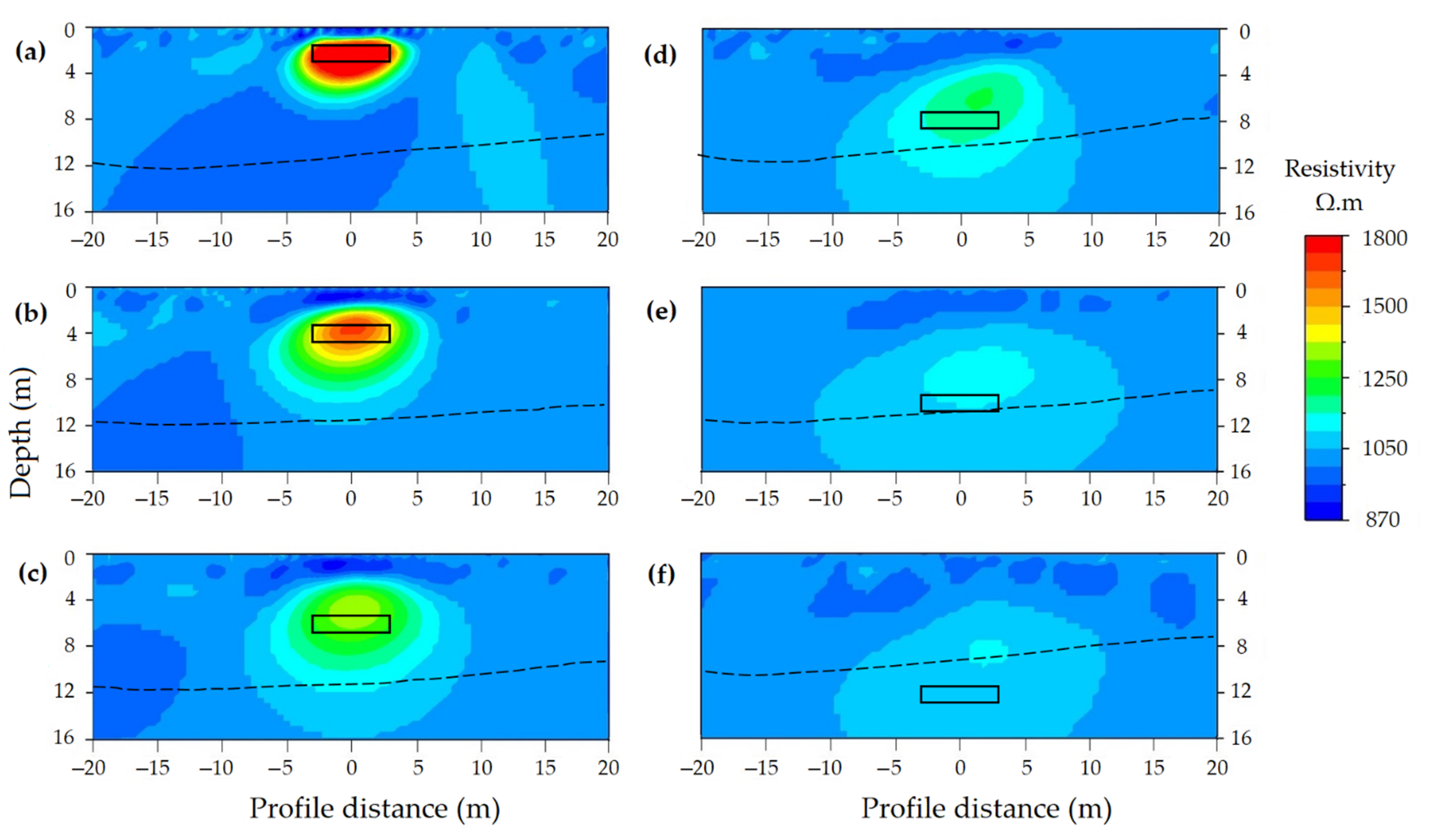
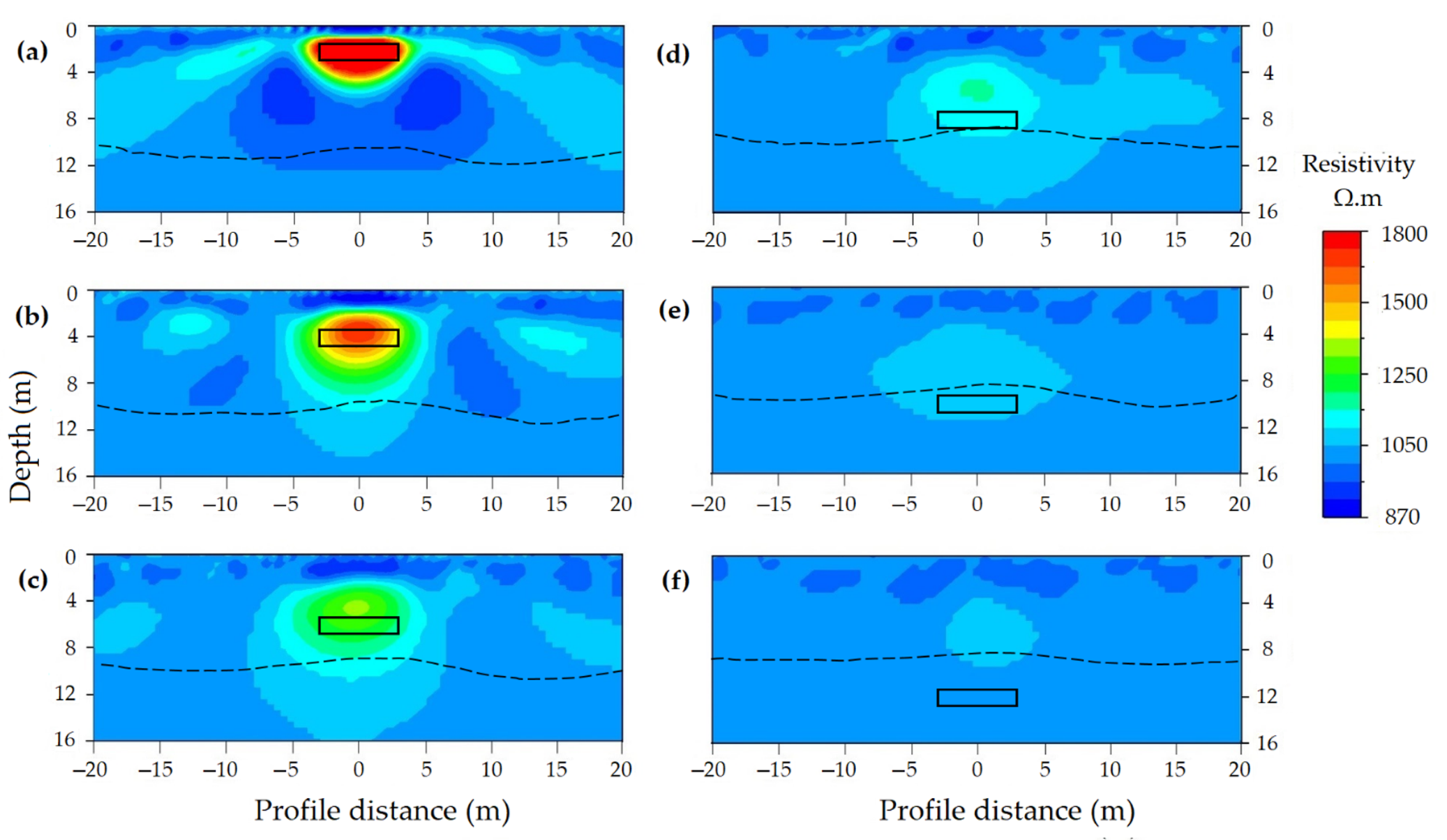
3.3.1. Model Accuracy
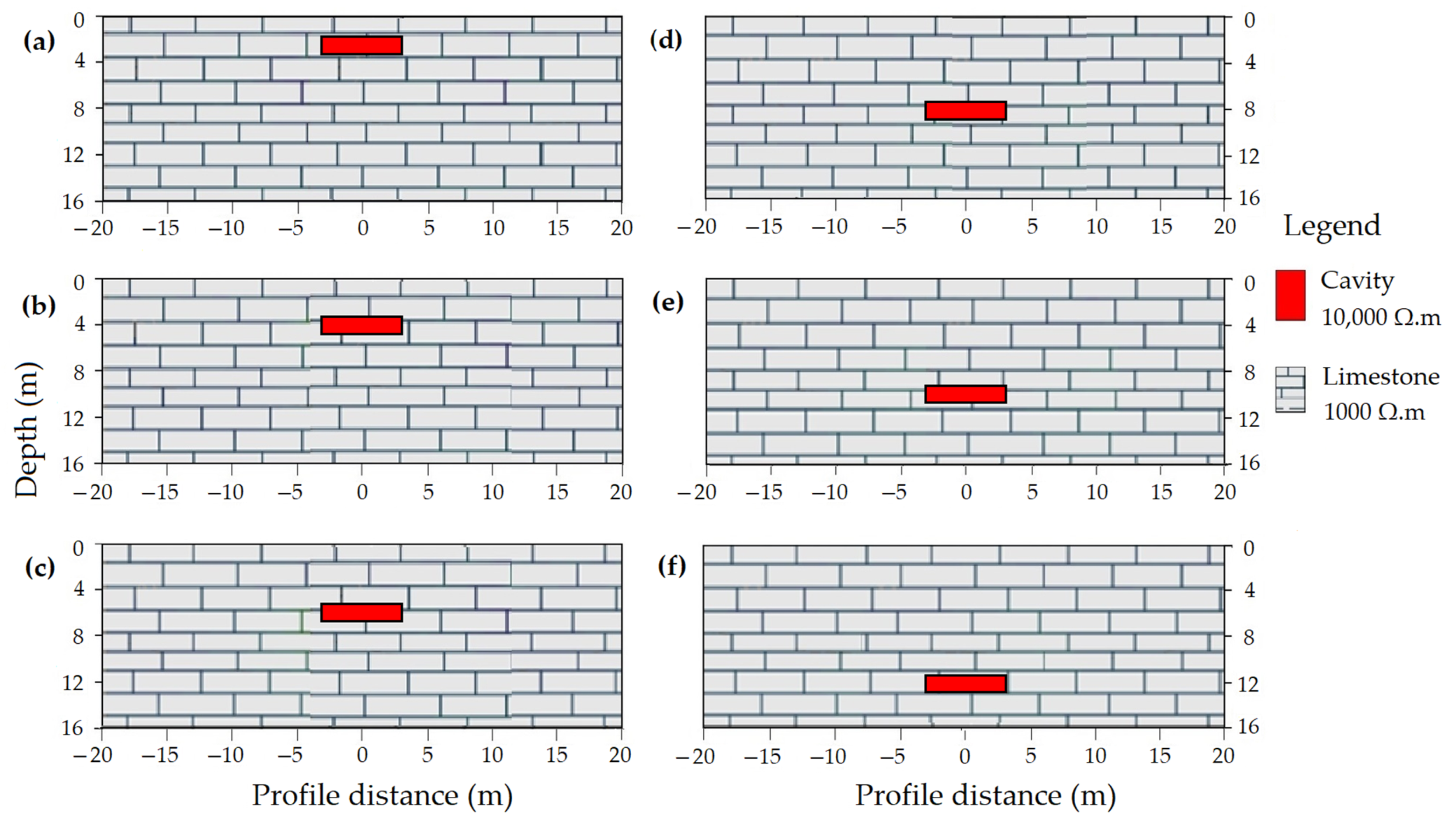
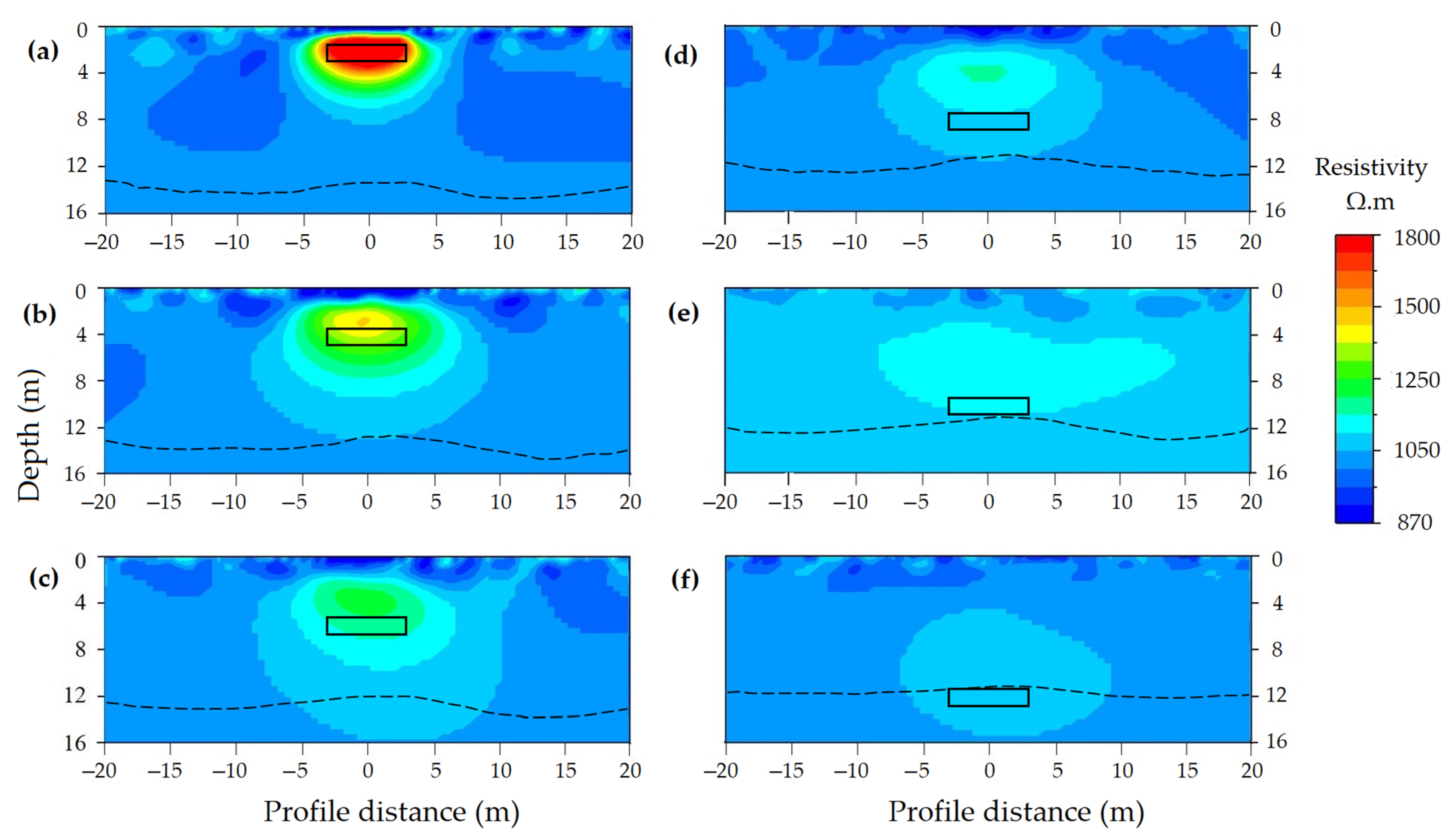
Depth of Cavity

We evaluated the model accuracy of arrays numerically using the image correlation between the actual and inverted resistivity models, as shown in Figure 6. The DD model correlation values were highest, varying from 0.29 (T6) to 0.82 (T1). On the other hand, the PD and WS models depicted moderate image correlation, ranging from 0.28 (T6) to 0.75 (T1) for the PD models and 0.24 (T6) to 0.81 (T1) for the WS models. The lowest correlation values were exhibited by the PP array, varying from 0.19 (T6) to 0.71 (T1). The correlation coefficients were directly associated with the accuracy of the obtained models.
Moreover, the cavity region showed significant changes in model accuracy and resolution based on cavity depth. For the convenience of description, we categorized the air-filled cavity targets as shallower (T1 and T2), intermediate (T3 and T4), and deeper (T5 and T6) based on the cavity situated depths.
The shallower cavity models situated at 2.2 m (T1) and 4.2 m (T2) depths were accurately reconstructed by the DD, PD, and WS arrays, as depicted in Figure 7, Figure 8 and Figure 9a,b. The obtained images have also shown a strong statistical correlation with actual models (Figure 6). The PP array yielded a relatively lower resolution than the tested arrays (Figure 10a,b). The resistivity imaging displayed relatively wider anomaly sizes regarding the actual cavity models (Figure 7, Figure 8, Figure 9 and Figure 10a,b). The obtained geometry accuracy was considerably varied for the upper and lower anomaly boundaries. For instance, the upper boundary of the T1 anomaly coincided with an actual cavity model, while the bottom boundary extended beyond that of the actual models (Figure 7a). Generally, inversion artefact increases with the survey depth; however, the inversion for high resistivity contrast may also provide a noticeable artefact, especially nearby the anomalous body [62]. Even though we applied the robust inversion algorithm, inversion for the shallow depth cavities has generated considerable artefacts, as depicted in Figure 7, Figure 8, Figure 9 and Figure 10a,b. The significant artefacts in inversions performed in all the air-filled cavity modeling had the resistivity value below 950 Ω·m, that is often misinterpreted as subsurface physical features.
Modeling for the intermediate cavities located at 6.2 m (T3) and 8.2 m (T4) depths showed reasonable model resolution in the tested arrays (Figure 7, Figure 8, Figure 9 and Figure 10c,d). The DD array displayed slightly better resolution than the other arrays. Figure 6 shows the moderate correlation between the inverted images and the actual models. The obtained anomaly sizes were noticeably overestimated, whereas the anomaly depths were underestimated by about 0.4–1.3 m with regard to actual cavity models. In Figure 7, Figure 8, Figure 9 and Figure 10c,d, the artefacts were clearly observed on the shallow part of the inverted models, particularly on the DD models. However, the resistivity imaging showed the intermediate cavity anomalies, the size overestimation and depth underestimation were limited the proper inference of the cavity information.
In contrast, the deeper cavity models set at 10.2 m (T5) and 12.2 m (T6) depths were not recovered adequately by any of the arrays (Figure 7, Figure 8, Figure 9 and Figure 10e,f). The obtained image correlations to the real model were weak (Figure 6). As shown in Figure 7, Figure 8, Figure 9 and Figure 10e,f, the anomaly sizes were highly overestimated, making it very challenging to interpret the cavity geometries without prior subsurface information. The result also showed about 1.6–3.0 m anomaly depth underestimation relative to the actual cavity locations. As the cavity depth increases, significant resistivity underestimation occurred in anomaly zones. Furthermore, the shallow parts of the final models were contaminated by patched inversion artefacts. These poor model accuracies can lead to inappropriate interpretation in resistivity imaging.
The anomaly responses of different arrays for a particular air-filled cavity were also examined graphically. We produced a one-dimensional (1D) horizontal resistivity profile from the inverted model of the cavity T2, which crossed the mid-point of the cavity at 4.2 m depth (as shown in Figure 11). We extracted the resistivity values along the 1D profile for the DD, PD, WS, and PP arrays. The DD array showed the highest (steepest) anomaly gradient over the cavity zone, with the peak resistivity value of 2220 Ω·m. In contrast, the PP array exhibited the lowest (gentlest) anomaly gradient, with the peak resistivity value of 1400 Ω·m. The 1D profile of the PD and WS arrays showed moderate anomaly gradients that have the peak resistivity value of 1850 and 1700 Ω·m, respectively. The arrays that provided the steep anomaly gradient can recover cavity boundaries more accurately, while the arrays that yield the gentle anomaly gradient prevent the inference of the cavity boundaries.
The 1D resistivity profiles were also used to assess the effect of air-filled cavity depth on the anomaly response of the arrays. Since the DD model provides the highest anomaly gradient, we used its models to generate 1D horizontal profiles for different depth cavity cases (Figure 12). The resistivity profile data were extracted along the profile lines that pass via the mid-points of the cavities T1, T2, T3, T4, T5, and T6 at depths of 2.2, 4.2, 6.2, 8.2, 10.2, and 12.2 m, respectively. The shallower cavity models showed a more robust resistivity amplitude than the cavity set at the relatively deeper position. For instance, the upper cavity T1 indicates the maximum anomaly amplitude with the peak resistivity value of 6470 Ω·m. In comparison, the bottom cavity T6 exhibits a minimum anomaly amplitude with a peak resistivity value of 1080 Ω·m. The substantial decrease in resistivity amplitude (gradient) as an increase in cavity depth can limit obtaining the anomaly geometries (Figure 12).
Furthermore, the depth of investigation (DOI) index may show variation based on the type of arrays and the resistivity distributions of the survey domain. We delineated the more reliable zones of the inverted models since higher credibility is given for the DOI patterns with values below 0.1 [28]. The zone below the threshold depth (DOI ≤ 0.1) is considered a low sensitive zone and assumed to be poorly imaged [63]. Air-filled cavity model simulation showed a small change of DOI index with cavity position, which is slightly shifted up as the cavity depth increases (Figure 7, Figure 8, Figure 9 and Figure 10). Consistent with our results, other studies [57] depicted the variation of DOI indexes based on the resistivity distribution of the survey domain. In our study, a significant variation of DOI index was also observed for different types of arrays. The inverted models have displayed the average DOI threshold depth of 8 m for DD, 9.8 m for WS, 10.5 m for PD, and 12.7 m for PP models (Figure 7, Figure 8, Figure 9 and Figure 10). For the same number of electrodes, equal spacing, and profile length, the largest DOI threshold depth shown by the PP array may be due to its greater penetration depth [22,25]. The PP array depicted the largest DOI threshold depth; however, it obtained the lowest model resolution with blurred cavity anomalies (Figure 10). This is likely related to the least sensitivity of the PP array to the subsurface resistivity variations [22,47].

Size of Cavity

The air-filled cavity size scenarios were used since the cavity size is an important factor in the array-model resolution. We used three cavity sizes as three scenarios: 0.5 × 6 m, 1.5 × 6 m, and 3 × 6 m respectively, all set at 4.2 m depth.
The cavity size significantly affects the resolution of the resistivity tomogram. The small cavity size in scenario 1 was not correctly resolved in any tested arrays; however, the DD array showed a relatively better result (Figure 13). The small size cavity can be highly smoothened by the inversion process, in addition to the low-resistivity measurement on the recording instrument that nearly approaches the host resistivity value (Figure 13). We show the results of scenario 2 with the results of the previous section for the similar-sized cavity T2 for the sake of comparison (Figure 14). Scenario 2 was adequately resolved in the DD, PD, and WS arrays; however, the PD and WS arrays’ resolution were slightly lower than the DD array, whereas the PP array poorly recovered the cavity in scenario 2. Moreover, all the tested arrays resolved scenario 3 cavities (Figure 15), but the PP array showed a relatively lower resolution than the other arrays. For increasing cavity size, the model resolution significantly improved, while the inversion artefacts considerably increased. The result showed that the overestimation in anomaly size was less pronounced as cavity size increases. By considering the homogenous host medium, cavity targets larger than the anomaly size in scenario 1 could be recovered effectively by the DD array. The DD and WS arrays could be effective for the cavity targets greater than or equal to the anomaly size in scenario 2. The PP array could be effective for the cavity size having a size greater than or equal to the anomaly in scenario 3.

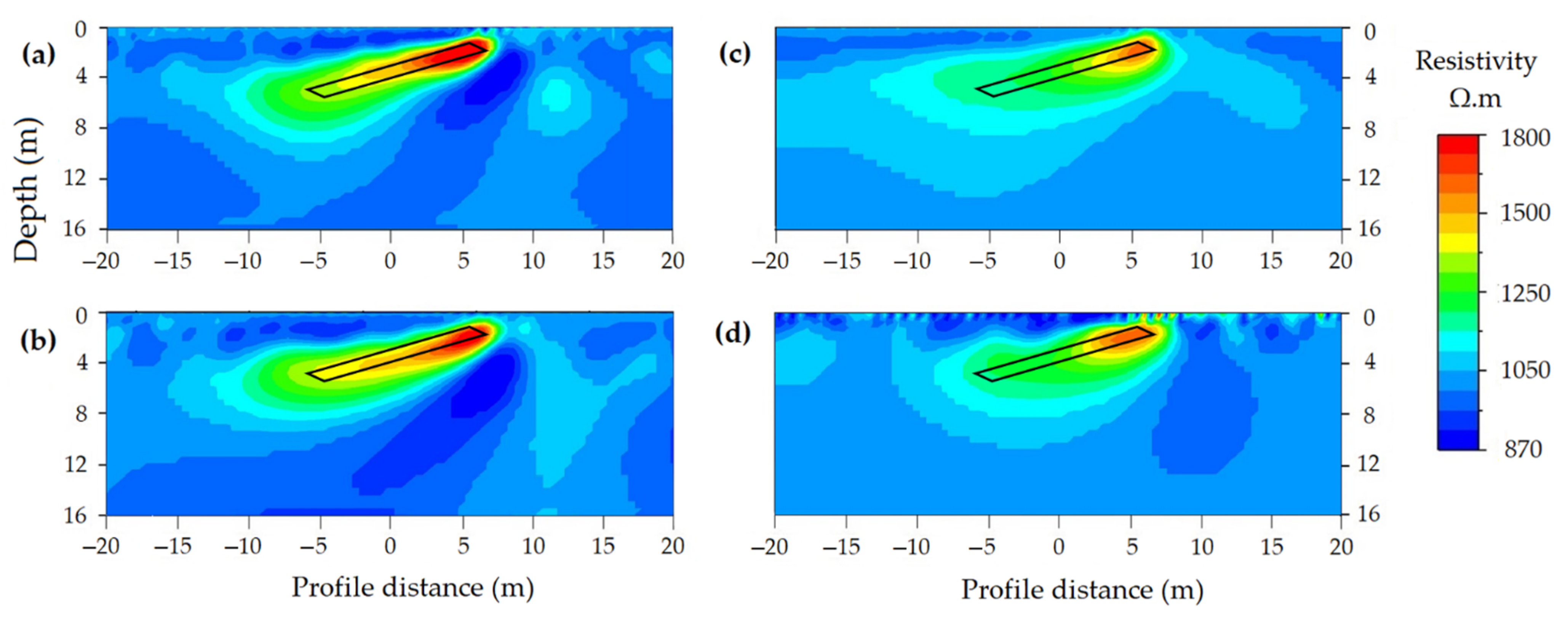
Orientation of Cavity
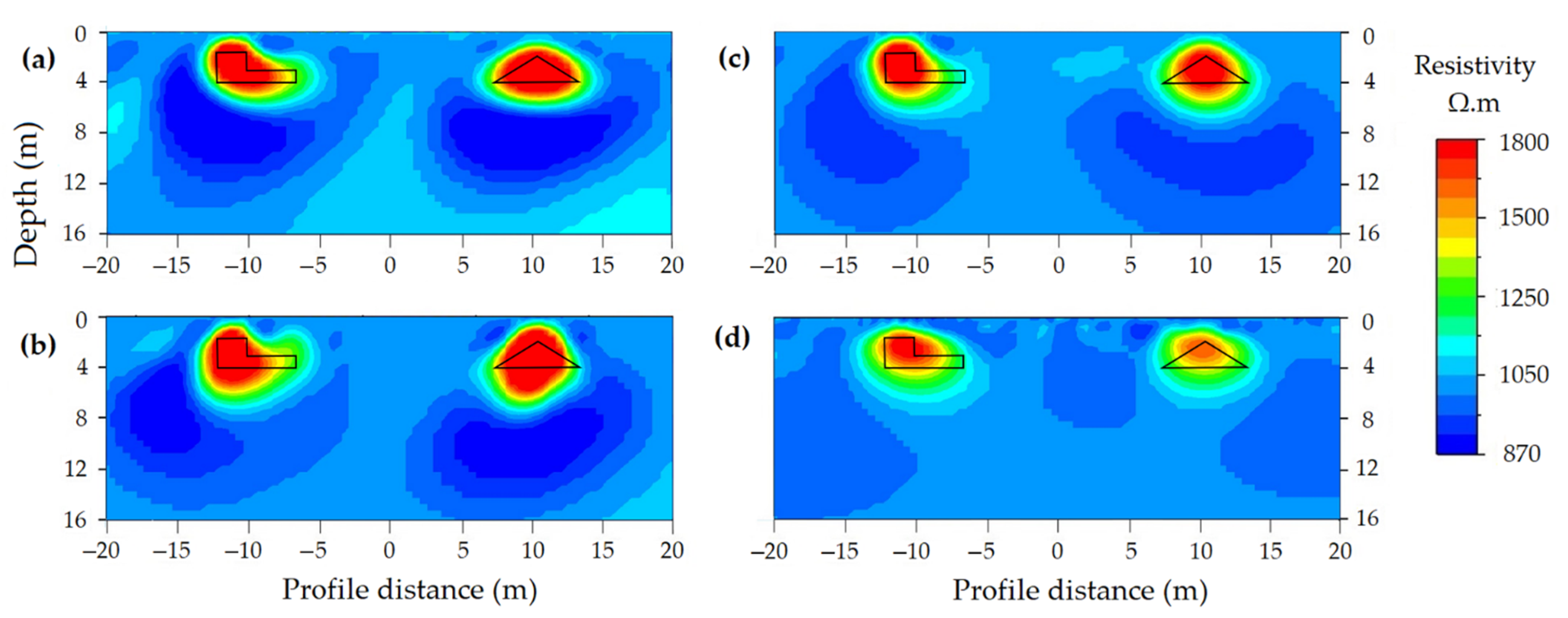
In karstic terrain, cavities are not usually aligned in the horizontal direction; thus, we examined the surface resistivity methods using a cavity target (0.5 × 6 m) set at a different inclination (I), such as the horizontal (I = 0°), inclined (I = 45°), and vertical (I = 90°). As the horizontal cavity models are discussed in the earlier sections (Figure 14), we present the inclined (Figure 16) and vertical (Figure 17) cavity models. The result showed that the orientation and geometry of the inclined cavity were correctly resolved in the DD and PD arrays. The WS and PP arrays recovered the upper part of the inclined cavity, but they did not properly detect the deeper parts (Figure 16). As shown in Figure 17, the PD and DD arrays also accurately recovered the orientation and geometry of the vertical cavity, whereas these were poorly reproduced in the WS and PP arrays. All the arrays recovered the geometry of the top cavity boundary since the resistivity method detected a high signal near the electrode position. For increasing cavity depth, the inverted resistivity value decreased, and the cavity anomaly width considerably increased. Pronounced inversion artefacts were observed in the inclined and vertical cavity models. It is well-known that the DD array is highly sensitive to the lateral variation of the subsurface structures [21,64]. However, our results show that the DD array can also resolve cavities oriented in the horizontal and inclined directions. The PD array could be more effective for vertical and inclined cavity structures compared to the horizontal structures. The WS array is known to be moderately sensitive to both lateral and vertical variations [22,27]. However, in our results, it showed relatively better resolution for the horizontal cavity than the inclined and vertical ones. The PP array depicted low resolution for all the tested orientations of the cavity.

Geometry of Cavity

Obtaining the exact geometry of the subsurface structure using the resistivity method is a challenging task [22,59]. As shown in Figure 18, we simulated two air-filled cavity geometries: the L-shaped cavity (left side) and the triangular-shaped cavity (right side). The L-shaped cavity geometry was slightly recovered in the DD and PD arrays. The WS and PP array did not reproduce the geometry of the L-shaped cavity. The shape of the triangular cavity was not reproduced in all the tested arrays. Even though the resistivity methods show a high anomaly over the buried cavity zone, its geometry cannot be adequately reconstructed for moderate to complex cavity structures. This is possibly associated with the smoothness effect of the inversion method [59].

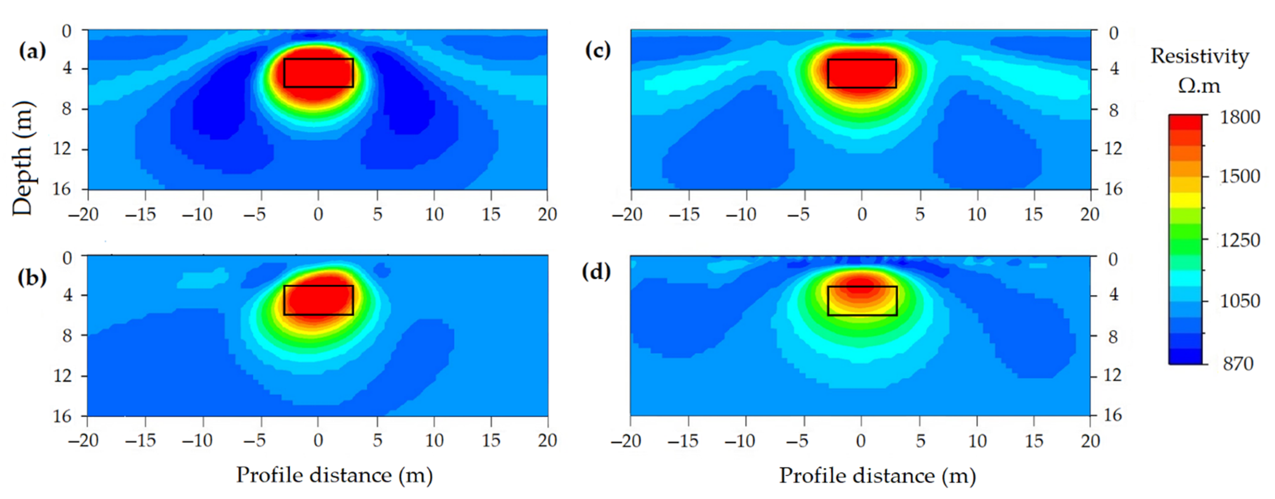
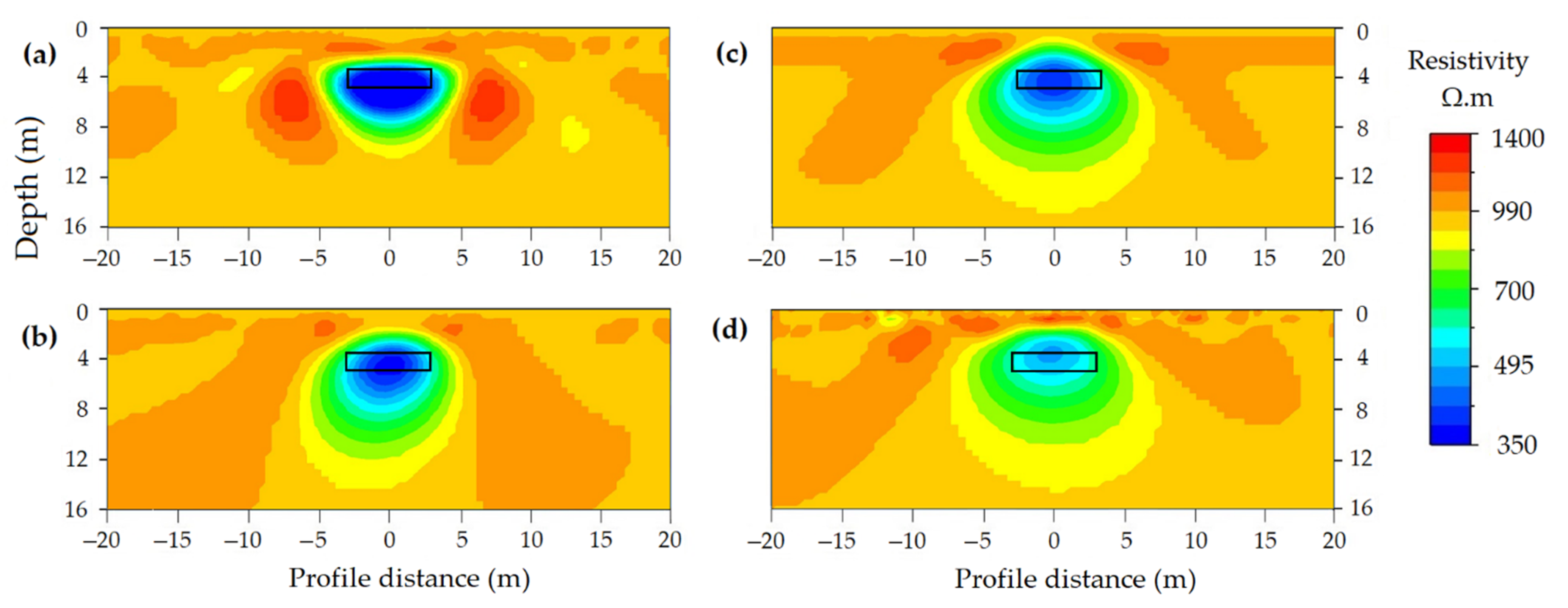
Conductive Cavity Modeling

The air-filled cavity showed a high anomaly in resistivity imaging, while a conductive cavity appeared as a low anomaly. For conductive cavity modeling, a cavity with a 1.5 × 6 m dimension set at 4.2 m depth was filled with dry clay (90 Ω·m) and saturated clay (50 Ω·m).
Figure 19 shows the inverted model results for a cavity filled with dry clay. The DD array accurately resolved the cavity; however, the anomaly size was higher than the actual cavity size. The PD and WS arrays also showed relatively high resolution, and their anomaly sizes were wider compared to the actual cavity. The recovered cavity orientation was tilted in the case of the PD array. The PP array showed the lowest resolution, and its anomaly geometry was unclear. The noticeable inversion artefact had a resistivity value above 1160 Ω·m that can lead to inappropriate model interpretation in resistivity studies. These artefacts were pronounced at shallow depth.
Significantly low resistivity may be detected in resistivity imaging over a cavity filled with clay and water [65]. We consider the groundwater level (2 m) above the cavity depth for the saturated clay-filled condition, as shown in Figure 20. The model inversion result showed that the saturated clay-filled cavity was accurately resolved in the DD array. The PD and WS arrays obtained high resolution; however, the WS array showed a slightly lower resolution than the PD array. The PP array identified the cavity zone, but its resolution is lower than the other arrays. All the arrays exhibited noticeably wider anomaly sizes with regard to the actual cavity size. The boundary between unsaturated and saturated limestone was precisely resolved in the DD, WS, and PP arrays, while the recovered boundary was slightly deeper in the PD array. The cavity filled with conductive materials showed a slight improvement in the resolution of cavity anomaly compared to the air-filled cavity model, particularly in the PP array (Figure 20). In line with our study, the DD array field study shows the highest resolution for the conductive cavity [21,66]. The numerical study for sinkhole modeling showed lower resolution in the DD array than the PD array, contradicting our study [33]. The field study for cavity detection displayed relatively high resolution in the PD array, while the PP array showed low resolution [67], consistent with our results.

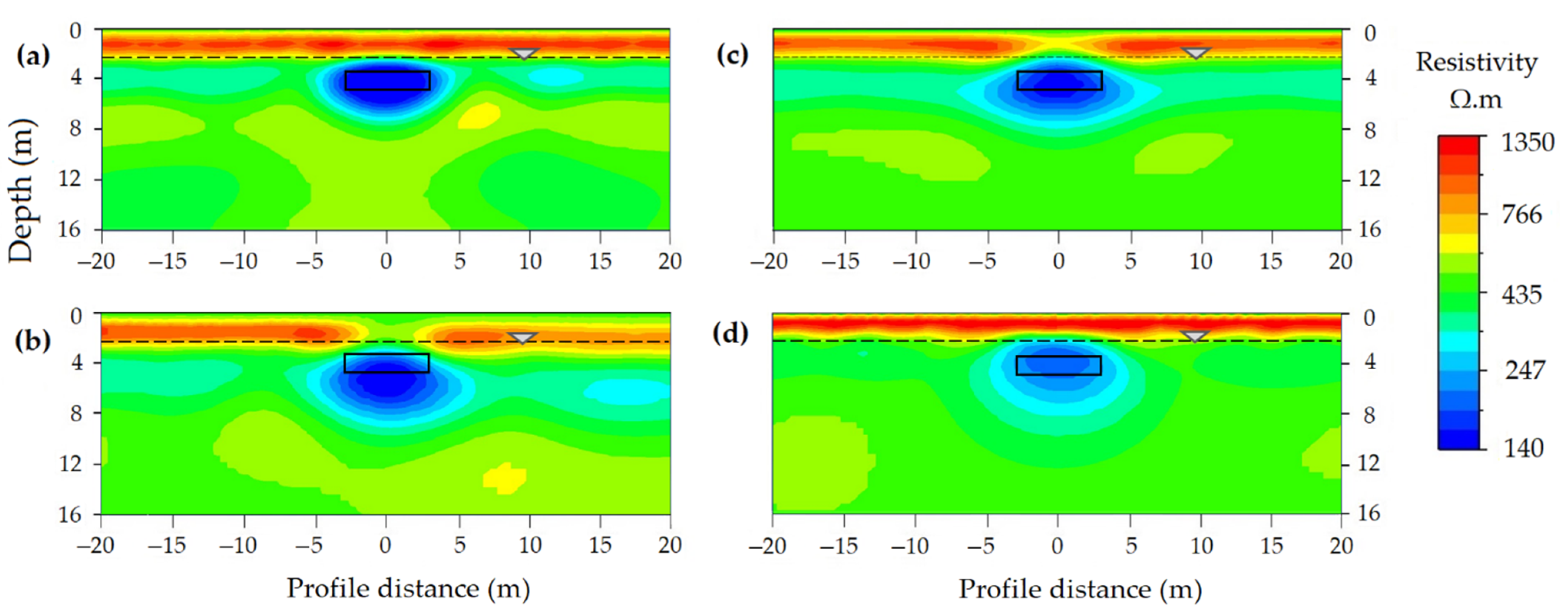
Experimental Cavity Study

A field experiment was also conducted to validate the numerical modeling results. Our numerical model cavities were embedded in a limestone unit; however, in the field experiment, we used moderately compacted sandy clay as the host unit around an empty plastic box which acted as the cavity (Figure 21). In our experiment, the one-tenth scale of the cavity target T2 was used. Thus, the plastic box’s center with 0.15 × 0.15 × 0.6 m size was situated at 0.42 m depth. The experimental resistivity datasets were measured using 89 electrodes of a 4-point light 10W (LGM Lippmann) resistivity meter with 0.1 m spacing (Figure 21).
Figure 22 shows the experimental resistivity survey results for the DD, PD, WS, and PP arrays. The DD and PD arrays showed a high resistivity anomaly at the cavity zone, whereas the lower anomaly amplitude was obtained by WS and PP arrays. The experimental cavity geometry was more adequately reconstructed in the DD and WS arrays; however, they obtained wider and shallower anomalies. The geometry of the cavity in the PD array was not properly restored—its left side anomaly was elongated to the greater depth. The PP array exhibited a triangular anomaly instead of providing the rectangular cavity shape. Compared to the numerical results, the experimental cavity anomaly in all the tested arrays showed considerable underestimation of anomaly depth. The depth underestimation in cavity studies can lead to inappropriate interpretation, similar to other field studies [26,68]. Since our study was conducted in shallow sandy clay, the patchily distributed high and low resistive features were inferred as the inversion artefacts. The DD, PD, and PP arrays artefact agreed with synthetic model results, whereas a relatively greater artefact was observed in the WS arrays. As the experimental cavity was set in low-resistive sandy clay, its obtained resistivity values were considerably underestimated compared to the numerical cavity, which was embedded in limestone rock. Based on the experimental result, the WS and DD arrays are more appropriate for the subsurface cavity study, whereas the PD array is reasonable. The PP array is the least suitable, particularly in obtaining the cavity geometry and position.
Our numerical and experimental study can help to decide proper arrays for subsurface target (e.g., cavity) studies. In line with our results, the field study and numerical modeling have shown that the DD array can accurately resolve the subsurface structures such as cavity [38,67], thin dike [25], buried wall [29,32], and sinkhole [21]. These structures were moderately recovered by the WS and PD arrays [24,26,69]. The pole-pole array is generally the poorest in terms of model accuracy and image quality [25,32], consistent with our study. The array effectiveness is also constrained by the target depth-to-dimension ratio [32]. In our results, the shallowest cavities with considerable size were recovered effectively (Figure 7, Figure 8, Figure 9 and Figure 10a). For example, the DD, WS, and PD arrays well recovered a cavity diameter larger than one-fourth times its depth, similar to other studies [24]. If the anomaly geometry is not considered, those arrays can detect relatively deeper cavities. Thus, the DD array could be the most effective, PD and WS arrays could be moderate, and the PP array could be the least effective for surveying subsurface targets such as environmental or archaeological features (e.g., buried cavity, tombs, and wall), and geological structures (e.g., dike and thin channels).

3.3.2. Spatial Resolution

The spatial resolution of resistivity imaging is a function of many factors, including subsurface material distribution, data accuracy, array sampling scheme, and the parameters used in the model (e.g., smoothing factors) [70,71]. In this study, we used three different anomaly sizes as input models with the same inversion parameters to assess the spatial resolution of the arrays (DD, PD, WS, and PP).
Figure 23 shows the resolution test for scenario 1 with a checkerboard cell size of 1 × 2 m. In this scenario, the DD array can resolve the anomalies in both rows; however, the resolution is significantly reduced for the second row. Other arrays can only resolve the top row of anomalies. The WS and PP arrays depicted smearing at selected locations, whereas the PD array showed vertical smearing across the profile. The anomaly geometries were not well resolved for the PD array.
The second scenario with a checkerboard cell size of 2 × 4 m was better resolved in general compared to scenario 1, as shown in Figure 24. The DD array was able to recover the first and second rows, but the resolution was slightly reduced for the second row. The PD and WS arrays restored the entire checkerboard anomalies for the first row; however, the resolution of the second row was significantly reduced. The PP array recovered only the first row, and its anomaly was considerably smeared. The geometries of the checkerboard patterns were more accurately recovered by the DD, PD, and WS arrays, while the geometries could not be reproduced correctly for the PP array.
The larger size of 4 × 8 m was considered in the third scenario, as shown in Figure 25. The DD array resolved the first and the second rows; however, the resolution was slightly reduced for the second row. The PD, WS, and PP arrays consistently imaged the first row input checkerboard structures, but these were not resolved correctly in the second row. The second row checkerboards’ geometry was not accurately recovered for all the arrays and displayed elongated checker anomalies instead of rectangular cells.
The checkerboard test results depicted that even though we used the same arrays, the resolution of the recovered anomalies can vary based on their sizes. In general, the checkerboard resolution test of the first scenario reproduced about 12.5% checkerboard patterns (Figure 23), while the second scenario (twice the size of scenario 1) restored about 25% of the checkerboard (Figure 24). The third scenario (twice the size of scenario 2) reproduced about 50% of the checkerboard patterns (Figure 25). Thus, the increase in target size can noticeably increase the obtained model resolution and recovery depth. If the uniform background resistivity anomaly has a low amplitude compared to the targeted anomaly, then the depth of recovery is higher (Figure 7). However, all the alternating anomalies have similar amplitudes in the checkerboard test (Figure 24), and the recovery depth is low. This is likely related to the concentration of current density at the first-row of the checkerboard, which significantly decreases with depth, as current density is concentrated at the top layer in stratified formation [72,73]. As the resistivity data points are not uniformly distributed in the profile section, the inverted model resolution can considerably be biased. As shown in Figure 23 and Figure 24, the center of the survey profiles is well recovered, but smearing is observed at the end of the profiles.
We can choose the best array type for surveying shallow subsurface features supporting the checkerboard resolution test with different studies if prior information is available. Among the tested arrays, the DD array could be the most appropriate method for studying concealed small-scale features with less than or equal to the checkerboard size in scenario 1, such as void, tombs, and thin dikes [26,33,68]. The geological or environmental structures (e.g., thin buried channels) with the checkerboard size in scenario 2 could be recovered effectively by the DD, PD, and WS arrays [25,30]. All the tested arrays could resolve the subsurface features (e.g., tunnels, sinkholes) having a size greater than or equal to the checkerboard size in scenario 3 [21,30]. These arrays could be more effective if the targets-embedded media are homogenous.

3.3.3. Sensitivity to Resistivity Contrasts

The detection of subsurface structure using the resistivity method is mainly dependent on resistivity contrast, which may constrain the inverted model resolution [16]. We used different resistivity perturbations (±20%, 40%, 60%, and 80%) to examine array (DD, PD, WS, and PP) sensitivities. As shown in Figure 26, the DD array can resolve the first two rows of the checkerboards for the tested perturbations. However, the model resolution of the DD array was considerably enhanced for increased resistivity perturbation, reflecting the high sensitivity of the DD array. The high sensitivity of the DD array helped to study various subsurface structures with low [25,74] to high [32,75] resistivity contrasts. In contrasts, the PD array recovered the first row of the checkerboard patterns (Figure 27); however, the anomaly sizes were significantly overestimated for the higher values of negative perturbations (−60% and −80%). It can slightly detect the positive 20% perturbation of the second-row checkerboards. The PD array resolution was slightly improved as the resistivity contrast increased, indicating the less sensitivity of the PD array to the resistivity perturbations. The WS array can recover the first row of the checkerboard anomalies in all the perturbations as well as high perturbations (60% and 80%) of the second row (Figure 28). However, the resolution of the WS array is relatively lower than the DD array, and its resolution considerably improved for the increased resistivity contrasts, indicating high sensitivity to resistivity perturbations. The PP array adequately reproduced the first-row checkerboards for all the perturbations. Its resolution slightly increased, but the improvements are negligible. This is likely related to the low sensitivity of the PP array for both low- and high-resistivity contrasts (Figure 29). As shown in Figure 26, Figure 27, Figure 28 and Figure 29, all the arrays recovered the first row of the checkerboard patterns for the tested resistivity perturbations. This may be associated with the high sensitivity of the resistivity methods near the vicinity of the electrode positions.
Furthermore, the checkerboard tests were used to assess the inversion artefacts. The extensive anomaly features observed below 2 m depth in Figure 23, below 4 m depth in Figure 24, Figure 26, Figure 27, Figure 28 and Figure 29, and below 8 m depth in Figure 25 were not in the input model and interpreted as inversion artefacts. The pronounced artefacts at the edge of the profiles (e.g., Figure 26) are likely related to limited data points or no data coverages [76]. As shown in Figure 26, Figure 27, Figure 28 and Figure 29, the artefact contaminations were slightly increased as the degree of resistivity perturbation increases, as the cross-borehole resistivity experiment for analyzing subsurface heterogeneity between two boreholes has also shown [70]. Even though the DD array has high resolving power, the recovered models were highly contaminated by the inversion artefacts (Figure 26). The PD and PP arrays produced moderate artefacts (Figure 27 and Figure 29), whereas the WS array showed smaller artefacts (Figure 28). The inversion artefacts show a linear association with signal-to-noise ratio; for instance, the low signal-to-noise ratio of the DD array correlates with greater artefacts and the high signal-to-noise ratio of the WS array correlates with lesser inversion artefacts [25,77].
We present the summary of the results from the experimental model and all the synthetic modeling performed in this study in Table 1. It can help readers to decide appropriate array types for the planned subsurface cavity studies.
In this study, we observed that a specific resistivity imaging method might provide varying model accuracy, resolution, and anomaly responses for inversion of a single cavity model situated at different survey depths. Such ambiguity in subsurface cavity studies can substantially be reduced by applying two or more geophysical methods. Various methods have different capabilities to resolve the subsurface structures; thus, they complement each other and obtain detailed subsurface information. The joint inversion of two separate datasets may improve the overall resolution and match the inverted and the actual model [78]. Moreover, the joint interpretation of different outputs from two or more geophysical methods can minimize model ambiguity [77]. For example, a joint interpretation of results from resistivity tomography and ground penetration radar survey can reduce the non-uniqueness of the inverted resistivity model. Particularly in cavity study, the upper and lower boundaries of the cavity will be clearly determined by high-resolution ground penetration radar; however, it usually fails to provide information about the host medium and the cavity-filling materials. Instead, the resistivity imaging quite well detects the cavity-filling materials and the surrounding formation, but it cannot resolve the accurate geometry of the cavity [19]. Hence, using a joint interpretation of the model results and performing a joint inversion of different methods can reduce those inherited uncertainties of the resistivity imaging.

4. Conclusions

This study examined the uncertainties of resistivity imaging and identified the efficient arrays for subsurface cavity studies. Different numerical examples were demonstrated to examine the depth, size, orientation, geometry, and filling material effects on the array’s imaging ability. An experimental cavity study was also performed to compare with the numerical model results. In addition, we studied the spatial resolution for different checkerboard sizes and assessed arrays’ sensitivities to resistivity perturbations. The conceptual models were simulated to generate apparent resistivity data. The detection abilities of the arrays were statistically analyzed using variances and anomaly effects of the synthetically measured resistivity data. The apparent resistivity data were inverted to recover geoelectric models, and the model accuracies were evaluated.
Based on cavity depth modeling, the DD array exhibited the highest anomaly effect (1.46) and variance (24,400 Ω·m) in measured resistivity data for the shallowest cavity (T1) set at 2.2 m depth. In contrast, the PP array showed the lowest anomaly effect (0.18) and variance (900 Ω·m) for the deeper cavity (T6) set at 12.2 m depth. The anomaly effect and the variance of resistivity data decreased for increasing cavity depths, limiting the recovery of the cavity information. The DOI threshold depths were delineated, and the inverted models were inspected. As cavity depth increases, the statistical image correlation between the inverted and actual models was significantly decreased. The anomaly sizes were considerably overestimated as cavity depth increases, which can highly restrict the recovery of accurate geometries.
The arrays’ spatial resolution was significantly reduced as the size of the checkerboard decreased. All the tested arrays accurately resolved the first row of the checkerboard cells, but the second-row cells were considerably smeared, especially in the WS, PD, and PP arrays. Based on sensitivity tests, all the arrays were highly sensitive to the resistivity contrasts at the vicinity to electrode location. The DD and WS arrays showed higher sensitivity to resistivity perturbations than the PD and PP arrays. The PD displayed slightly better sensitivity compared to the PP array. Considerable artefact contaminations occurred for the DD, PD, and PP models, whereas minor contamination was observed on the WS models, which correlates with the signal-to-noise ratios of these arrays.
The study identified the ideal subsurface target probing arrays based on model accuracy, resolution, and sensitivity. We infer that the DD array is the most effective for studying subsurface targets (e.g., cavity), the PD and WS arrays are adequate, whereas the PP array is the least suitable for target probing. The sensitivity and resolution were substantially reduced as the depth increased; thus, a single cavity set at varying depth resulted in different solutions. This leads to ambiguity in model interpretations of the resistivity method. Under these circumstances, integrating prior information, performing a joint inversion of different parameters, and jointly interpreting the model outputs of two or more methods can significantly reduce the inherent uncertainties of the resistivity method.

Author Contributions

Y.G.D. was responsible for data analysis, simulations, and writing the draft. P.-Y.C. supervised and instructed results analysis and modified the manuscript. J.M.P. provided comments on results discussions with the other two authors. All authors have read and agreed to the published version of the manuscript.

Funding

This research was funded by the Minister of Science and Technology (MOST) of Taiwan under the project number of MOST 108-2638-E-008-001-MY2. This research was also partly supported by Earthquake-Disaster, Risk Evaluation and Management Centre, E-DREaM, from the Featured Areas Research Centre Program within the framework of the Higher Education Sprout Project by the Ministry of Education (MOE) in Taiwan.

Institutional Review Board Statement

Not applicable.

Informed Consent Statement

Not applicable.

Data Availability Statement

Data will be available upon request to the authors.

Acknowledgments

We would like to thank Partul Ranjan for his valuable revision and idea. We are grateful to Yitea Seneshaw for proofreading and comments. We also thank Shie Meng-Shiun, Ding-Jiun Lin, Yoseph Arba, and Lingerew Nebere, who contributed to experimental data collection. The comments and suggestions from anonymous reviewers have significantly improved the paper.

Conflicts of Interest

The authors declare no conflict of interest.

References

  1. Chang, P.-Y.; Chang, L.-C.; LEE, T.-Q.; Chan, Y.-C.; Chen, H.-F. Examining Lake-bottom structures with the resistivity imaging method in Ilan’s Da-Hu Lake in Northeastern Taiwan. J. Appl. Geophy. 2015, 119, 170–177. [Google Scholar]
  2. Fazzito, S.Y.; Rapalini, A.E.; Cortés, J.M.; Terrizzano, C.M. Characterization of Quaternary faults by electric resistivity tomography in the Andean Precordillera of Western Argentina. J. S. Am. Earth Sci. 2009, 28, 217–228. [Google Scholar] [CrossRef]
  3. Ho, G.-R.; Chang, P.Y.; Lo, W.; Liu, C.-M.; Song, S.-R. New evidence of regional geological structures inferred from reprocessing and resistivity data interpretation in the Chingshui-Sanshing-Hanchi area of Southwestern Ilan County, NE Taiwan. Terr. Atoms. Ocean Sci. 2014, 25, 491. [Google Scholar] [CrossRef] [Green Version]
  4. Tsai, J.P.; Chang, P.Y.; Yeh, T.C.J.; Chang, L.C.; Hsiao, C.T. Constructing the Apparent Geological Model by Fusing Surface Resistivity Survey and Borehole Records. J. Groundw. 2019, 57, 590–601. [Google Scholar] [CrossRef]
  5. Caputo, R.; Piscitelli, S.; Oliveto, A.; Rizzo, E.; Lapenna, V. The use of electrical resistivity tomographies in active tectonics: Examples from the Tyrnavos Basin, Greece. J. Geodyn. 2003, 36, 19–35. [Google Scholar] [CrossRef]
  6. Chang, P.-Y.; Chang, L.-C.; Hsu, S.-Y.; Tsai, J.-P.; Chen, W.-F. Estimating the hydrogeological parameters of an unconfined aquifer with the time-lapse resistivity-imaging method during pumping tests: Case studies at the Pengtsuo and Dajou sites, Taiwan. J. Appl. Geophy. 2017, 144, 134–143. [Google Scholar] [CrossRef]
  7. Zhang, G.; Zhang, G.-B.; Chen, C.-C.; Chang, P.-Y.; Wang, T.-P.; Yen, H.-Y.; Dong, J.-J.; Ni, C.-F.; Chen, S.-C.; Chen, C.-W. Imaging rainfall infiltration processes with the time-lapse electrical resistivity imaging method. Pure Appl. Geophys. 2016, 173, 2227–2239. [Google Scholar] [CrossRef]
  8. Chang, P.-Y.; Chen, C.-c.; Chang, S.-K.; Wang, T.-B.; Wang, C.-Y.; Hsu, S.-K. An investigation into the debris flow induced by Typhoon Morakot in the Siaolin Area, Southern Taiwan, using the electrical resistivity imaging method. Geophys. J. Int. 2012, 188, 1012–1024. [Google Scholar] [CrossRef] [Green Version]
  9. Drahor, M.G.; Göktürkler, G.; Berge, M.A.; Kurtulmuş, T.Ö. Application of electrical resistivity tomography technique for investigation of landslides: A case from Turkey. J. Environ. Geol. 2006, 50, 147–155. [Google Scholar] [CrossRef]
  10. Gómez-Ortiz, D.; Martín-Velázquez, S.; Martín-Crespo, T.; De Ignacio-San José, C.; Lillo, J. Application of electrical resistivity tomography to the environmental characterization of abandoned massive sulphide mine ponds (Iberian Pyrite Belt, SW Spain). Near Surf. Geophys. 2010, 8, 65–74. [Google Scholar] [CrossRef] [Green Version]
  11. Cardarelli, E.; Cercato, M.; Cerreto, A.; Di Filippo, G. Electrical resistivity and seismic refraction tomography to detect buried cavities. Geophys. Prospect. 2010, 58, 685–695. [Google Scholar] [CrossRef]
  12. Van Schoor, M. Detection of sinkholes using 2D electrical resistivity imaging. J. Appl. Geophy. 2002, 50, 393–399. [Google Scholar] [CrossRef] [Green Version]
  13. Gabarrón, M.; Martínez-Pagán, P.; Martínez-Segura, M.A.; Bueso, M.C.; Martínez-Martínez, S.; Faz, Á.; Acosta, J.A.J.M. Electrical resistivity tomography as a support tool for physicochemical properties assessment of near-surface waste materials in a mining tailing pond (El Gorguel, SE Spain). Minerals 2020, 10, 559. [Google Scholar] [CrossRef]
  14. Batayneh, A.T. Archaeogeophysics–archaeological prospection–A mini review. J. King Saud Univ. Sci. 2011, 23, 83–89. [Google Scholar] [CrossRef] [Green Version]
  15. Mochales, T.; Casas, A.; Pueyo, E.; Pueyo, O.; Román, M.; Pocoví, A.; Soriano, M.; Ansón, D. Detection of underground cavities by combining gravity, magnetic and ground penetrating radar surveys: A case study from the Zaragoza area, NE Spain. Environ. Geol. 2008, 53, 1067–1077. [Google Scholar] [CrossRef]
  16. Das, P.; Mohanty, P.R. Resistivity imaging technique to delineate shallow subsurface cavities associated with old coal working: A numerical study. Environ. Earth Sci. 2016, 75, 661. [Google Scholar] [CrossRef]
  17. Loke, M.; Barker, R. Practical techniques for 3D resistivity surveys and data inversion. Geophys. Prospect. 1996, 44, 499–523. [Google Scholar] [CrossRef]
  18. Sharma, S.; Verma, S. Solutions of the inherent problem of the equivalence in direct current resistivity and electromagnetic methods through global optimization and joint inversion by successive refinement of model space. Geophys. Prospect. 2011, 59, 760–776. [Google Scholar] [CrossRef]
  19. Orlando, L. GPR to constrain ERT data inversion in cavity searching: Theoretical and practical applications in archeology. J. Appl. Geophy. 2013, 89, 35–47. [Google Scholar] [CrossRef]
  20. Narayan, S.; Dusseault, M.B.; Nobes, D.C. Inversion techniques applied to resistivity inverse problems. Inverse Probl. 1994, 10, 669. [Google Scholar] [CrossRef] [Green Version]
  21. Zhou, W.; Beck, B.F.; Adams, A.L. Effective electrode array in mapping karst hazards in electrical resistivity tomography. J. Environ. Geol. 2002, 42, 922–928. [Google Scholar] [CrossRef]
  22. Loke, M. Tutorial: 2-D and 3-D Electrical Imaging Surveys; Geotomo Software: Penang, Malaysia, 2004. [Google Scholar]
  23. Yang, X.; Lagmanson, M.B. Planning resistivity surveys using numerical simulations. In Proceedings of the 16th EEGS Symposium on the Application of Geophysics to Engineering and Environmental Problems, San Antonio, TX, USA, 6–10 April 2003; p. cp-190-00047. [Google Scholar]
  24. Santos, F.A.M.; Afonso, A.R.A. Detection and 2D modelling of cavities using pole–dipole array. J. Environ. Geol. 2005, 48, 108–116. [Google Scholar] [CrossRef]
  25. Dahlin, T.; Zhou, B. A numerical comparison of 2D resistivity imaging with 10 electrode arrays. Geophys. Prospect. 2004, 52, 379–398. [Google Scholar] [CrossRef] [Green Version]
  26. Amini, A.; Ramazi, H. CRSP, numerical results for an electrical resistivity array to detect underground cavities. Open Geosci. 2017, 9, 13–23. [Google Scholar] [CrossRef] [Green Version]
  27. Martinez-Lopez, J.; Rey, J.; Duenas, J.; Hidalgo, C.; Benavente, J. Electrical Tomography Applied to the Detection of Subsurface Cavites. J. Caves Karst Stud. 2013, 75, 28–37. [Google Scholar] [CrossRef]
  28. Oldenburg, D.W.; Li, Y. Estimating depth of investigation in dc resistivity and IP surveys. Geophysics 1999, 64, 403–416. [Google Scholar] [CrossRef]
  29. Martorana, R.; Fiandaca, G.; Casas Ponsati, A.; Cosentino, P. Comparative tests on different multi-electrode arrays using models in near-surface geophysics. J. App. Geophy. 2009, 6, 1–20. [Google Scholar] [CrossRef] [Green Version]
  30. Hassan, A.A.; Kadhim, E.H.; Ahmed, M.T. Performance of Various Electrical Resistivity Configurations for Detecting Buried Tunnels Using 2D Electrical Resistivity Tomography Modelling. Diyala J. Eng. Sc. 2018, 11, 14–21. [Google Scholar] [CrossRef]
  31. Rezaei, S.; Shooshpasha, I.; Rezaei, H. Reconstruction of landslide model from ERT, geotechnical, and field data, Nargeschal landslide, Iran. Bull. Eng. Geol. Environ. 2019, 78, 3223–3237. [Google Scholar] [CrossRef]
  32. Eissa, R.; Cassidy, N.; Pringle, J.; Stimpson, I. Electrical resistivity tomography array comparisons to detect cleared-wall foundations in brownfield sites. Q. J. Eng. Geol. 2020, 53, 137–144. [Google Scholar] [CrossRef]
  33. Park, M.K.; Park, S.; Yi, M.-J.; Kim, C.; Son, J.-S.; Kim, J.-H.; Abraham, A.A. Application of electrical resistivity tomography (ERT) technique to detect underground cavities in a karst area of South Korea. Environ. Earth Sci. 2014, 71, 2797–2806. [Google Scholar] [CrossRef]
  34. Neyamadpour, A.; Wan Abdullah, W.; Taib, S.; Neyamadpour, B. Comparison of Wenner and dipole–dipole arrays in the study of an underground three-dimensional cavity. J. App. Geophy. 2010, 7, 30–40. [Google Scholar] [CrossRef]
  35. Boschi, L. Measures of resolution in global body wave tomography. Geophys. Res. Lett. 2003, 30. [Google Scholar] [CrossRef]
  36. Mewes, B.; Hilbich, C.; Delaloye, R.; Hauck, C. Resolution capacity of geophysical monitoring regarding permafrost degradation induced by hydrological processes. Cryosphere 2017, 11, 2957–2974. [Google Scholar] [CrossRef] [Green Version]
  37. Butler, D.J.N.-S.G.; Activity, H. Detection and characterization of subsurface cavities, tunnels and abandoned mines. Near Surf. Geophys. Hum. Act. 2008, 578–584. [Google Scholar]
  38. Satitpittakul, A.; Vachiratienchai, C.; Siripunvaraporn, W. Factors influencing cavity detection in Karst terrain on two-dimensional (2-D) direct current (DC) resistivity survey: A case study from the western part of Thailand. Eng. Geol. 2013, 152, 162–171. [Google Scholar] [CrossRef]
  39. Smith, R.C.; Sjogren, D.B. An evaluation of electrical resistivity imaging (ERI) in Quaternary sediments, southern Alberta, Canada. Geosphere 2006, 2, 287–298. [Google Scholar] [CrossRef] [Green Version]
  40. Keller, G.V.; Carmichael, R. Electrical properties of rocks and minerals. CRC Handb. Phys. Prop. Rocks 1982, 1, 217–293. [Google Scholar]
  41. Lowrie, W.; Fichtner, A. Fundamentals of Geophysics; Cambridge University Press: Cambridge, UK, 2020. [Google Scholar]
  42. Zhao, D.; Hasegawa, A.; Kanamori, H. Deep structure of Japan subduction zone as derived from local, regional, and teleseismic events. J. Geophys. Res. Solid Earth 1994, 99, 22313–22329. [Google Scholar] [CrossRef]
  43. Zhao, D.; Yanada, T.; Hasegawa, A.; Umino, N.; Wei, W. Imaging the subducting slabs and mantle upwelling under the Japan Islands. Geophys. J. Int. 2012, 190, 816–828. [Google Scholar] [CrossRef] [Green Version]
  44. Zhang, Y.; Wang, B.; Lin, G.; Ouyang, Y.; Wang, T.; Xu, S.; Song, L.; Wang, R. Three-Dimensional P-wave Velocity Structure of the Zhuxi Ore Deposit, South China Revealed by Control-Source First-Arrival Tomography. Minerals 2020, 10, 148. [Google Scholar] [CrossRef] [Green Version]
  45. Athanasiou, E.; Tsourlos, P.; Papazachos, C.; Tsokas, G. Combined weighted inversion of electrical resistivity data arising from different array types. J. App. Geophy. 2007, 62, 124–140. [Google Scholar] [CrossRef]
  46. Günther, T. Inversion Methods and Resolution Analysis for the 2D/3D reconstRuction of Resistivity Structures from DC Measurements; Universitätsbibliothek der TU BAF: Freiberg, Germany, 2005. [Google Scholar]
  47. Okpoli, C.C. Sensitivity and resolution capacity of electrode configurations. Geophys. J. Int. 2013, 2013, 608037. [Google Scholar] [CrossRef] [Green Version]
  48. Oldenborger, G.A.; Routh, P.S.; Knoll, M.D. Sensitivity of electrical resistivity tomography data to electrode position errors. Geophys. J. Int. 2005, 163, 1–9. [Google Scholar] [CrossRef] [Green Version]
  49. AGI. Instruction Manual for EarthImager™ 2D Version 2.4. 0.; Advanced Geosciences, Inc.: Austin, TX, USA, 2009. [Google Scholar]
  50. Rubin, Y.; Hubbard, S.S. Hydrogeophysics; Springer Science & Business Media: Berlin/Heidelberg, Germany, 2006; Volume 50. [Google Scholar]
  51. Wolke, R.; Schwetlick, H. Iteratively reweighted least squares: Algorithms, convergence analysis, and numerical comparisons. SIAM J. Sci. Comput. 1988, 9, 907–921. [Google Scholar] [CrossRef]
  52. Degroot-Hedlin, C.; Constable, S. Occam’s inversion to generate smooth, two-dimensional models from magnetotelluric data. Geophysics 1990, 55, 1613–1624. [Google Scholar] [CrossRef]
  53. Ren, Z.; Kalscheuer, T. Uncertainty and resolution analysis of 2D and 3D inversion models computed from geophysical electromagnetic data. Surv. Geophys. 2020, 41, 47–112. [Google Scholar] [CrossRef] [Green Version]
  54. Militzer, H.; Rösler, R.; Lösch, W. Theoretical and experimental investigations for cavity research with geoelectrical resistivity methods. Geophys. Prospect. 1979, 27, 640–652. [Google Scholar] [CrossRef]
  55. Aizebeokhai, A.; Olayinka, A. Anomaly effects of arrays for 3d geoelectrical resistivity imaging using orthogonal or parallel 2d profiles. Afr. J. Environ. Sci. Technol. 2010, 4, 446–454. [Google Scholar]
  56. Chai, T.; Draxler, R.R. Root mean square error (RMSE) or mean absolute error (MAE)–Arguments against avoiding RMSE in the literature. Geosci. Model Dev. 2014, 7, 1247–1250. [Google Scholar] [CrossRef] [Green Version]
  57. Hilbich, C.; Marescot, L.; Hauck, C.; Loke, M.; Mäusbacher, R. Applicability of electrical resistivity tomography monitoring to coarse blocky and ice-rich permafrost landforms. Permafr. Periglac. Process. 2009, 20, 269–284. [Google Scholar] [CrossRef] [Green Version]
  58. Yang, X.; Chen, X.; Carrigan, C.R.; Ramirez, A.L. Uncertainty quantification of CO2 saturation estimated from electrical resistance tomography data at the Cranfield site. Int. J. Greenh. Gas Control. 2014, 27, 59–68. [Google Scholar] [CrossRef] [Green Version]
  59. Portniaguine, O.; Zhdanov, M.S. Focusing geophysical inversion images. Geophysics 1999, 64, 874–887. [Google Scholar] [CrossRef] [Green Version]
  60. Hauck, C.; Mühll, D.V. Inversion and interpretation of two-dimensional geoelectrical measurements for detecting permafrost in mountainous regions. Permafr. Periglac. Process. 2003, 14, 305–318. [Google Scholar] [CrossRef]
  61. Olayinka, A.; Yaramanci, U.; Geophysics, E. Choice of the best model in 2-D geoelectrical imaging: Case study from a waste dump site. Eur. J. Environ. Sci. 1999, 3, 221–244. [Google Scholar]
  62. Carey, A.M.; Paige, G.B.; Carr, B.J.; Dogan, M.J. Forward modeling to investigate inversion artifacts resulting from time-lapse electrical resistivity tomography during rainfall simulations. J. Appl. Geophy. 2017, 145, 39–49. [Google Scholar] [CrossRef]
  63. Caterina, D.; Beaujean, J.; Robert, T.; Nguyen, F. A comparison study of different image appraisal tools for electrical resistivity tomography. Near Surf. Geophys. 2013, 11, 639–658. [Google Scholar] [CrossRef]
  64. Seaton, W.J.; Burbey, T.J. Evaluation of two-dimensional resistivity methods in a fractured crystalline-rock terrane. J. Appl. Geophy. 2002, 51, 21–41. [Google Scholar] [CrossRef]
  65. Kim, J.-H.; Yi, M.-J.; Hwang, S.-H.; Song, Y.; Cho, S.-J.; Synn, J.-H. Integrated geophysical surveys for the safety evaluation of a ground subsidence zone in a small city. J. Geophys. Eng. 2007, 4, 332–347. [Google Scholar] [CrossRef]
  66. Festa, V.; Fiore, A.; Parise, M.; Siniscalchi, A.; Studies, K. Sinkhole evolution in the Apulian karst of southern Italy: A case study, with some considerations on sinkhole hazards. J Caves Karst Stud. 2012, 74, 137–147. [Google Scholar] [CrossRef]
  67. Muhammad, F.; Samgyu, P.; Young, S.S.; Ho Kim, J.; Mohammad, T.; Adepelumi, A.A. Subsurface cavity detection in a karst environment using electrical resistivity (er): A case study from yongweol-ri, South Korea. Earth Sci. Res. J. 2012, 16, 75–82. [Google Scholar]
  68. Saribudak, M.; Hawkins, A.; Stoker, K. Do air-filled caves cause high resistivity anomalies? A six-case study from the Edwards Aquifer Recharge Zone in San Antonio, Texas. Houst. Geol. Soc. Bull. 2012, 54, 41–49. [Google Scholar]
  69. Gourdol, L.; Clément, R.; Juilleret, J.; Pfister, L.; Hissler, C. Large-scale ERT surveys for investigating shallow regolith properties and architecture. Hydrol. Earth Syst. Sci. Discuss. 2018, 2018, 1–39. [Google Scholar]
  70. Nimmer, R.E.; Osiensky, J.L.; Binley, A.M.; Williams, B.C. Three-dimensional effects causing artifacts in two-dimensional, cross-borehole, electrical imaging. J. Hydrol. 2008, 359, 59–70. [Google Scholar] [CrossRef]
  71. Daily, W.; Ramirez, A. Electrical resistance tomography during in-situ trichloroethylene remediation at the Savannah River Site. J. Appl. Geophy. 1995, 33, 239–249. [Google Scholar] [CrossRef]
  72. Verdet, C.; Anguy, Y.; Sirieix, C.; Clément, R.; Gaborieau, C. On the effect of electrode finiteness in small-scale electrical resistivity imaging. Geophysics 2018, 83, EN39–EN52. [Google Scholar] [CrossRef]
  73. Rucker, D.F.; Loke, M.H.; Levitt, M.T.; Noonan, G.E. Electrical-resistivity characterization of an industrial site using long electrodes. Geophysics 2010, 75, WA95–WA104. [Google Scholar] [CrossRef]
  74. Hermawan, O.R.; Putra, D.P.E. the effectiveness of wenner-schlumberger and dipole-dipole array of 2d geoelectrical survey to detect the occurring of groundwater in the gunung kidul karst aquifer system, Yogyakarta, Indonesia. J. Appl. Geol. 2016, 1, 71–81. [Google Scholar] [CrossRef] [Green Version]
  75. Andrej, M.; Uros, S.; Studies, K. Electrical Resistivity Imaging of Cave Divaska Jama, Solvania. J. Caves Karst. Stud. 2012, 74, 235–242. [Google Scholar] [CrossRef]
  76. Dahlin, T.; Loke, M.H. Resolution of 2D Wenner resistivity imaging as assessed by numerical modelling. J. Appl. Geophy. 1998, 38, 237–249. [Google Scholar] [CrossRef] [Green Version]
  77. Adepelumi, A.; Fayemi, O. Joint application of ground penetrating radar and electrical resistivity measurements for characterization of subsurface stratigraphy in Southwestern Nigeria. J. Geophys. Eng. 2012, 9, 397–412. [Google Scholar] [CrossRef]
  78. Gallardo, L.A.; Meju, M.A. Joint two-dimensional DC resistivity and seismic travel time inversion with cross-gradients constraints. J. Geophys. Res. Solid Earth 2004, 109. [Google Scholar] [CrossRef]
Figure 1. Resistivity synthetic models that represent a target cavity set in limestone unit at six different depths: (a) Target cavity T1 at 2.2 m, (b) target cavity T2 at 4.2 m, (c) target cavity T3 at 6.2 m, (d) target cavity T4 at 8.2 m, (e) target cavity T5 at 10.2 m, (f) target cavity T6 at 12.2 m depth. The depth indicates the mid-point of the cavity. For better illustration, we presented only 40 m horizontal section of the models.
Applsci 11 03143 g001
Figure 2. The variance of the numerically measured resistivity data for air-filled cavity situated at different survey depths.
Applsci 11 03143 g002
Figure 3. The anomaly effect of the arrays with regard to the air-filled cavity survey depths.
Applsci 11 03143 g003
Figure 4. The scatter plot of the model predicted and synthetically measured apparent resistivity data for the arrays: (a) dipole-dipole (DD) array, (b) pole-dipole (PD) array, (c) Wenner–Schlumberger (WS) array, and (d) pole-pole (PP) array. Overestimated and underestimated data outliers are displayed on the upper and lower boundaries.
Applsci 11 03143 g004
Figure 5. Arrays’ inversion error for varying air-filled cavity depths.
Applsci 11 03143 g005
Figure 6. The statistical correlation between the inverted resistivity models and actual air-filled cavity models.
Applsci 11 03143 g006
Figure 7. The inverted resistivity model using dipole-dipole (DD) array for the cavity targets: (a) T1, (b) T2, (c) T3, (d) T4, (e) T5, (f) T6. The rectangular boxes indicate the actual air-filled cavities. The broken lines represent the depth of investigation (DOI) threshold depths. For better anomaly illustration, we presented only a 40 m lateral model section.
Applsci 11 03143 g007
Figure 8. The inverted resistivity model using pole-dipole (PD) array for the cavity targets: (a) T1, (b) T2, (c) T3, (d) T4, (e) T5, (f) T6. The rectangular boxes indicate the actual air-filled cavities. The broken lines represent the DOI threshold depths.
Applsci 11 03143 g008
Figure 9. Inverted resistivity model using Wenner–Schlumberger (WS) array for the cavity targets: (a) T1, (b) T2, (c) T3, (d) T4, (e) T5, (f) T6. The rectangular boxes indicate the actual air-filled cavities. The broken lines represent the DOI threshold depths.
Applsci 11 03143 g009
Figure 10. Inverted resistivity model using pole-pole (PP) array for the cavity targets: (a) T1, (b) T2, (c) T3, (d) T4, (e) T5, (f) T6. The rectangular boxes indicate the actual air-filled cavities. The broken lines represent the DOI threshold depths.
Applsci 11 03143 g010
Figure 11. Resistivity anomaly gradient of the arrays for the target cavity T2.
Applsci 11 03143 g011
Figure 12. Resistivity anomaly gradient for the air-filled cavity set at different survey depths using the dipole-dipole (DD) array.
Applsci 11 03143 g012
Figure 13. The inverted resistivity model for scenario 1 with 0.5 × 6 m cavity size using: (a) DD array, (b) PD array, (c) WS array, (d) PP array. The rectangular box indicates the actual cavity target.
Applsci 11 03143 g013
Figure 14. The inverted resistivity model for scenario 2 with 1.5 × 6 m cavity size using: (a) DD array, (b) PD array, (c) WS array, (d) PP array. The rectangular box indicates the actual cavity target.
Applsci 11 03143 g014
Figure 15. The inverted resistivity model for scenario 3 with 3 × 6 m cavity size using: (a) DD array, (b) PD array, (c) WS array, (d) PP array. The rectangular box indicates the actual cavity target.
Applsci 11 03143 g015
Figure 16. The inverted resistivity model for the inclined (45°) cavity using: (a) DD array, (b) PD array, (c) WS array, (d) PP array. The box indicates the actual cavity target.
Applsci 11 03143 g016
Figure 17. The inverted resistivity model for the vertical (90°) cavity size using: (a) DD array, (b) PD array, (c) WS array, (d) PP array. The rectangular box indicates the actual cavity target.
Applsci 11 03143 g017
Figure 18. The inverted resistivity models for the cavity geometries using: (a) DD array, (b) PD array, (c) WS array, (d) PP array. The solid line indicates the actual cavity targets.
Applsci 11 03143 g018
Figure 19. The inverted resistivity model for a cavity filled with dry clay using: (a) DD array, (b) PD array, (c) WS array, (d) PP array. The rectangular box indicates the actual cavity target.
Applsci 11 03143 g019
Figure 20. The inverted resistivity model for the saturated clay-filled cavity using: (a) DD array, (b) PD array, (c) WS array, (d) PP array. The rectangular box indicates the actual cavity target. The broken line represents the actual groundwater level.
Applsci 11 03143 g020
Figure 21. The experimental data collection procedure for resistivity imaging.
Applsci 11 03143 g021
Figure 22. The inverted resistivity model of the experimental data for the: (a) DD array, (b) PD array, (c) WS array, (d) PP array. The rectangular box indicates the buried empty plastic box.
Applsci 11 03143 g022
Figure 23. Scenario 1 spatial resolution test for the 1 m (vertical) × 2 m (horizontal) checkerboard cell sizes. (a) Checkerboard model, (b) DD array, (c) PD array, (d) WS array, (e) PP array.
Applsci 11 03143 g023
Figure 24. Scenario 2 spatial resolution test for the 2 m (vertical) × 4 m (horizontal) checkerboard cell sizes. (a) Checkerboard model, (b) DD array, (c) PD array, (d) WS array, (e) PP array.
Applsci 11 03143 g024
Figure 25. Scenario 3 spatial resolution test for the 4 m (vertical) × 8 m (horizontal) checkerboard cell sizes. (a) Checkerboard model, (b) DD array, (c) PD array, (d) WS array, (e) PP array.
Applsci 11 03143 g025
Figure 26. Dipole-dipole (DD) array sensitivity to resistivity perturbations. The inverted model for: (a) ±20% perturbation, (b) ±40% perturbation, (c) ±60% perturbation, (d) ±80% perturbation.
Applsci 11 03143 g026
Figure 27. Pole-dipole (PD) array sensitivity to resistivity perturbations. The inverted model for: (a) ±20% perturbation, (b) ±40% perturbation, (c) ±60% perturbation, (d) ±80% perturbation.
Applsci 11 03143 g027
Figure 28. Wenner–Schlumberger (WS) array sensitivity to resistivity perturbations. The inverted model for: (a) ±20% perturbation, (b) ±40% perturbation, (c) ±60% perturbation, (d) ±80% perturbation.
Applsci 11 03143 g028
Figure 29. Pole-pole (PP) array sensitivity to resistivity perturbations. The inverted model for: (a) ±20% perturbation, (b) ±40% perturbation, (c) ±60% perturbation, (d) ±80% perturbation.
Applsci 11 03143 g029
Table 1. Adequacy of the resistivity imaging types for cavity study: highly effective = xxx, moderately effective = xx, and less effective = x.
Adequacy of Arrays for CavityDDPDWSPP
Shallow depth (≲4 m) 1xxxxxxxxxxx
Intermediate depth (≲8 m and >4 m) 1xxxxx
Deeper depth (>8 m) 1xxx-
Small size (≲0.5 m) 2x---
Intermediate size (≲3 m and >0.5 m) 2xxxxxxxx
Large size (>3 m) 2xxxxxxxxxxx
Horizontal cavity 1,2xxxxxxxx
Vertical cavity 1xxxxxx
Inclined cavity 1xxxxxxxx
Dry clay-filled cavity 1,2xxxxxxx
Saturated clay-filled cavity 1,2xxxxxxxxxxx
1 Considering a 1.5 × 6 m cavity size. 2 Considering 4.2 m depth. Except for dry and saturated clay, all the scenarios considered an air-filled cavity. The host medium is considered as homogenous limestone. For the heterogeneous background, the checkerboard cell size scenarios could be used.
Publisher’s Note: MDPI stays neutral with regard to jurisdictional claims in published maps and institutional affiliations.

