Abstract
A novel method named residual-variational mode decomposition (RVMD) is proposed in this study to extract bearing fault features accurately. RVMD can determine the number of modes and the balance parameter adaptively, and it has two stages. In the first stage, the signal is decomposed into a series of modes until the correlation coefficient between the raw signal and the decomposition results reaches the threshold. A redefined kurtosis, which can resist the interferences from aperiodic impulse efficiency, is applied to rebuild the ensemble kurtosis index. The mode that has the largest rebuild-ensemble kurtosis, and its neighbors, are kept. By putting the residual signal into the second stage, an iteration process is applied to determine the optimal parameters for variational mode decomposition (VMD). VMD is re-run with the optimal parameters, and the sub-mode filtered with the larger rebuild-ensemble kurtosis is examined by the envelope analysis technology to observe the fault feature. The effectiveness of RVMD is verified by the simulation signal and three experiment signals. Its superiority is shown by comparing it with some existing methods.
1. Introduction
Rotation equipment has been widely used in modern industries, such as land transportation, ocean shipping, airlift, and some power transmission fields [1,2,3,4]. Although its strength and lifespan have been considered in the design stage, heavy loads and a terrible operating environment may accelerate the operating area deterioration (i.e., the interface between rolling elements and raceways in bearing and the meshing surface of two gears). Recent studies show the effectiveness of vibration signals in fault diagnosis [5,6]. Fault response of bearing and gearbox plays as impact component in vibration signal [7,8]. However, impulse response from the early fault is often submerged by noise from other running components and environments, given that the impulse response is too weak. Thus, an effective impulse signal detection method is necessary to evaluate the rotation machine’s operating status.
Many methods, like envelope analysis [9,10], empirical mode decomposition (EMD) [11,12], wavelet transform (WT) [13,14], and ensemble EMD (EEMD) [15,16], have been applied to extract impulse component from a heavy noise signal. Envelope analysis can detect impulse signals effectively but is weak in low signal-to-noise ratio (SNR) data. WT works well in heavy noise signals but is greatly limited by the basic function [17]. EMD and EEMD can decompose complex signals into server modals adaptively but they lack rigorous mathematical theory. VMD can decompose low SNR signals into server modes under suitable modal numbers and balance parameters [18]. Wang et al. [19] studied the filter property of VMD by simulation signal and found that it could be used to detect impulse signals. Wang et al. [20] detected impulse components in a signal from a rotor system using VMD. The comparison results among VMD, EMD, and EEMD indicated that VMD worked better than the other two methods. Li et al. [21] analyzed the signal from wind turbines by combining VMD and blind-source separation to detect the bearing crack fault. Li et al. [22] introduced VMD to calculate the central frequency and combined it with data-driven time-frequency analysis to diagnose gear fault. Some other articles [23,24,25] also examined VMD in the fault diagnosis field.
To sum up, VMD has been widely applied in the fault detection field. However, the above articles determined the number of modes and the balance parameter on the basis of experience. To solve this problem, Zhang et al. [26] applied a grasshopper optimization algorithm to determine the optimal parameters for VMD by maxing correlation coefficient kurtosis. Miao et al. [27] proposed to optimize ensemble kurtosis (EK) and improved the frequency-band estimation process. In this method, the criterion EK may be partial to the kurtosis in the envelope spectrum due to the absence of a high-frequency part in it. VMD combined with an intelligent algorithm works well, but the computational complexity is high, given that VMD has to be executed for each agent.
Some researchers proposed adaptive VMD from other perspectives, which can be parted into three aspects. First, the modal number is determined by the Fourier spectrum of a signal. Li et al. [28] proposed an independence-oriented VMD on the basis of the spectrum distribution to detect wheelset-bearing faults. Using this method, they determined a modal number using the number of the local maximum of the fast Fourier transform (FFT) spectrum. Thus, this method cannot work well when the signal’s FFT spectrum is complex and often leads to over-decomposition. Jiang et al. [29] proposed an initial center frequency-guided VMD, in which the center frequency was determined by the energy fluctuation spectrum. This method may strike if the energy fluctuation function is interfaced with heavy noise. Second, the modal number is determined by the characteristics of each sub-modal. For example, Lian et al. [30] proposed an adaptive VMD on the basis of the permutation entropy, the extreme value of spectrum, and kurtosis of each sub-modal, which is a complex method and has many parameters that need to be determined artificially. Gong et al. [31] proposed a tentative VMD (TVMD) method to diagnose the bearing fault. The stop criterion was the order of difference for the two sub-modes which had the largest kurtosis and came from the two adjacent modal number decomposition results. In this method the criterion was kurtosis, which was vulnerable to random impulses. Finally, a coarse-to-fine process was proposed to determine parameters for VMD [32]. In this method, the modal number was set as one, and the noise sub-modal was subtracted in each iteration. The stop criterion was based on the theoretical frequency and the kurtosis of the sub-modal. Accordingly, prior information was necessary for this method, and the impulse signal evaluation criterion was too crude. On the basis of the above descriptions, some problems remain to be solved, such as VMD without an intelligent algorithm and a suitable criterion for impulse signals.
A novel method called residual-VMD (RVMD) is proposed in the current study to fill the above gaps. RVDM is designed to have two stages. In the first stage, the balance parameter is set as 1000 following previous studies [26,29]. The modal number is initialized as one and increases gradually until the relationship correlation between the input and decomposition results reaches the threshold. A new kurtosis, which is redefined on the basis of the number of elements whose values are above the root mean square (RMS) of the squared data, is applied to rebuild EK which can effectively evaluate the ratio of the periodic impulses in each mode. By keeping the mode with the largest new EK, and its neighbors, the VMD has two modes in the second stage. An iteration process is also applied to determine the optimal balance parameter. After obtaining the optimal balance parameter, the VMD is re-run with it. The sub-mode with the larger new EK is analyzed by envelope analysis technology to observe the fault feature. The effectiveness of the proposed method is examined by simulation and experiment signals. The comparison results among three other methods indicate the superiority of the proposed method.
2. Proposed Method
In this section, we introduce the basic theory about VMD and redefine kurtosis. Then, the proposed method will be built upon the basis of them.
2.1. Basic Theory of VMD
In this study, VMD is applied to extract the impulse component from the noise signal. VMD, compared with EMD and EEMD, has a solid theoretical basis. It can decompose multi-component signals into a series of sub-modes by some adaptive Wiener filter banks. In VMD, the output can be written as solving a constrained variational problem. The equation can be presented as:
where denotes the modal number, and denotes the center frequency of each sub-modal . Usually, Lagrangian multipliers and penalty technology are applied to transform Equation (1) into an unconstrained problem. Thus, Equation (1) can be written as:
where denotes the balance parameter, which can affect the bandwidth of . Here denotes the Lagrangian multiplier parameter. In VMD, Equation (2) is solved by the alternate direction method of multipliers (ADMM) technology. Thus, the sub-modal and its corresponding center frequency will be updated as:
Then, the remained Lagrangian multiplier can be updated by:
Finally, the stop criterion of ADMM is shown as:
On the basis of the introduction of VMD, the modal number and balance parameter go through the whole process of VMD. Thus, suitable parameters should be selected for VMD.
2.2. Redefined Kurtosis
A suitable evaluation criterion of impulsive signals for fault diagnosis is extremely important. One of the most common measurements is kurtosis. Research [27] combined the kurtosis of time-domain data and the kurtosis in the squared envelope spectrum (SES) to evaluate impulse signals. This method is known as ensemble kurtosis (EK). The kurtosis of SES can improve the ability of anti-interference impulses but still inherits the drawbacks of kurtosis. In the current study, kurtosis is redefined and the new kurtosis is applied to EK to build a new index for the evaluation of periodic impulses. Consequently, the new index has stronger power to resist interferences from aperiodic impulses than the traditional EK.
Kurtosis can be calculated as:
which can be written as:
In this study, is assumed constant. If only one element is not zero in , then will be equal to zero, and the kurtosis of the data will be the largest. The kurtosis of the data will decrease if two elements are not zero in . For large interference impulses, this situation can be set as only one non-zero element in . Thus, the kurtosis will be very large, and our judgment may be distorted by it. To overcome this drawback, we redefine kurtosis as:
where is defined as the ratio of the number of elements whose values are above a specific threshold to the data length. Generally, the threshold can be defined as the mean of the data. However, the RMS of is applied in this study because of two reasons. First, each of the data is squared in Equation (10). Thus, the data are reasonably evaluated as . Second, the RMS can reflect the large aperiodic impulses more effectively than the mean. The relationship between the RMS and the mean can prove this reason. For a digital signal, their relationship can be written as:
where is the RMS, and is the mean. Here is the waveform factor, which can be defined as:
where T is the period of the pulse wave, and t is the corresponding duration. An example for introducing the two parameters is shown in Figure 1.
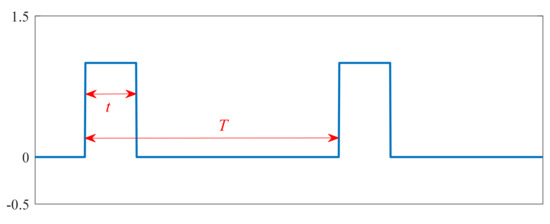
Figure 1.
The flowchart of IEFI-MVMD.
Here will increase with the decrease in , as shown in Figure 1. For some large aperiodic impulses, they can be simulated by pulse waves with a small and large . Thus, for the large aperiodic impulses has a big value.
On the basis of Equation (12), can be calculated as:
Based on Equation (14), it is easy to understand that RMS can reflect large impulses more efficiently than the mean. For a large RMS, the number of these elements whose values are above it will be small. Thus, the kurtosis defined by Equation (11) can effectively suppress the interferences from aperiodic impulses. In this study, the number of this kind of elements is defined as . Thus, Equation (11) can be written as:
The new kurtosis defined above is applied to calculate the ensemble kurtosis defined in [27]. The new ensemble kurtosis can be calculated as:
where SEK and K are the new kurtosis of the SES and time-domain data, respectively.
2.3. RVMD
A novel method named RVMD is proposed in this study to extract the impulsive component accurately. RVMD is designed to have two stages. The first stage is to roughly find the impulses, and the second stage is to determine the impulses. The main steps of RVMD can be summarized as follows:
Step 1: Initialize system parameters: and .
Step 2: Run the VMD and compute the correlation coefficient () between the raw signal and the decomposition result. If , proceed to Step 3. Otherwise, let and repeat Step 2.
Step 3: Compute for each mode. The residual signal is determined as follows: if the largest is the first or the last mode, the residual signal is obtained by adding the mode that has the largest with its neighbor mode. Otherwise, the residual signal will be obtained by adding the mode with the largest with its right and left neighbors.
Step 4: Fix and run VMD with . Compute for each . Repeat Step 4 until .
Step 5: Run VMD with the optimal parameters, which correspond to the largest . The sub-mode with the larger is analyzed by the envelope analysis technology to show the fault feature.
The flowchart of the proposed method is presented in Figure 2.
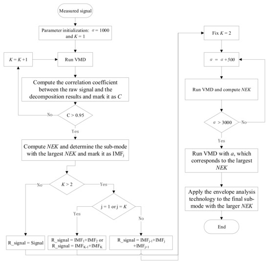
Figure 2.
The flowchart of RVMD.
3. Simulation and Case Study
3.1. Simulation Analysis
The simulation signal includes the harmonic component (), the periodic impulse (), the aperiodic impulse (), and the Gaussian noise (). The simulation signal can be written as:
In the simulation signal, the frequency of the impulse signal is set as . The sampling frequency is 20 kHz, and the length of the simulation signal is 10 k. The density of Gaussian noise is 0.4. The simulation signal is shown in Figure 3, and its SES is shown in Figure 4. As Figure 4 shows, it is difficult to find the feature frequency due to the existence of interferences from Gaussian noise and aperiodic impulses.
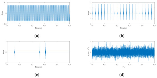
Figure 3.
Simulation signal: (a) harmonic component , (b) periodic impulse component , (c) interface impulse component , and (d) composite signal .
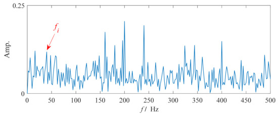
Figure 4.
SES of the simulation signal.
The proposed method was applied to analyze this signal, and the results are shown in Figure 5 and Figure 6. The time-domain waveform (TDW) shown in Figure 5b includes some periodic impulses, consistent with the results shown by NEK. The SES of the sub-mode shown in Figure 5b is presented in Figure 6. The fundamental frequency and its harmonics are clearly shown in it. Thus, the proposed method can effectively extract the periodic impulse features and it has a strong resistance against the interferences from the aperiodic impulses.
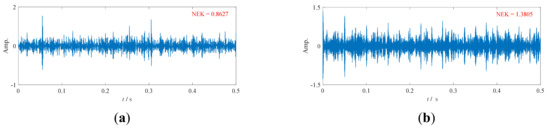
Figure 5.
Results by RVMD for the simulation signal: (a) IMF1 and (b) IMF2.
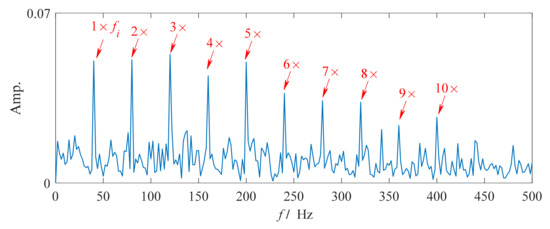
Figure 6.
SES of the result shown in Figure 5b.
3.2. Case I
In this section, the proposed method is applied to analyze some signals from the bearing fault experiment. The signals used in this section are obtained from the Society for Machinery Failure Prevention Technology (MFPT) [33]. On the basis of the description in [33], the fault kind of the test bearing includes outer and inner race fault conditions. The ball pass frequency on the inner race (BPFI) is 118 Hz, and the ball pass frequency on the outer race (BPFO) is 81 Hz with a test speed of 25 Hz. The sampling frequency is 48,828 Hz, and the data length applied in this section is 1 s. The information on the raw signal is displayed in Figure 7.
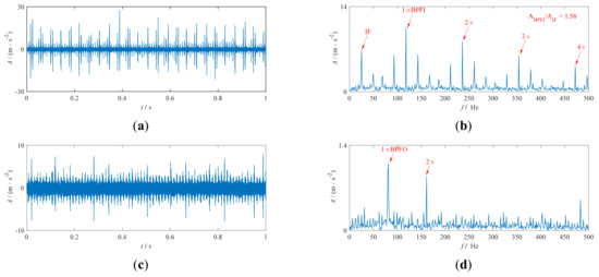
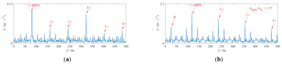
Figure 7.
Signals from MFPT: (a,b) correspond to the TDW and SES of the inner race fault bearing; (c,d) correspond to the TDW and SES of the outer race fault bearing.
Then, the proposed method is applied to process this signal, and the results are shown in Figure 8 and Figure 9. The second sub-mode of the results from the RVMD for the inner race fault signal has the larger NEK, as shown in Figure 8. Accordingly, it should be processed by envelope analysis technology. On the basis of the results from the outer race fault signal, the first sub-mode should be analyzed further, and their results are shown in Figure 9. The results shown in Figure 9a are extremely similar to the raw SES shown in Figure 7b. To describe the differences clearly, the ratio of the largest amplitudes between the fault feature frequency and interference frequency (IF) is applied in this study. A larger ratio means a better fault feature extraction result. Based on the ratios shown in the two figures, we can say the inner race fault feature is efficiently enhanced by our method. By comparing the results shown in Figure 7d and Figure 9b, only the primary fault frequency and 2× can be found in the raw SES, but the primary fault frequency, 2×, 3×, 4×, 5×, and 6× can be found from the result by the proposed method. Consequently, RVMD can efficiently extract the bearing fault feature.
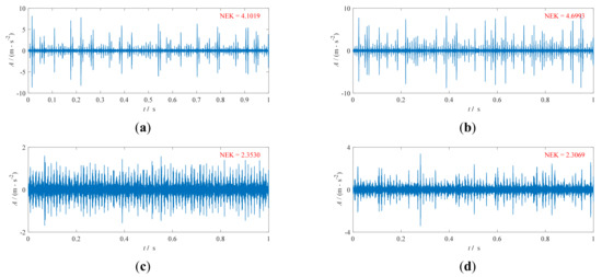
Figure 8.
Results by the RVMD for the signals from MFPT: (a,b) correspond to the first and second sub-modes of the inner race fault bearing; (c,d) correspond to the first and second sub-modes of the outer race fault bearing.
These signals are also processed by some other methods, including fast kurtogram (FK), ICF-VMD, and RVMD with the traditional kurtosis, to show the superiority of the proposed method. Figure 10 displays the results by FK. From Figure 10a, the optimal demodulation frequency band (ODFB) for the inner fault race signal is in level 3.5 with a center frequency of 21,362 Hz. The corresponding SES based on it is shown in Figure 10b. From it, we can see the fault is weakened by FK, which is consistent with the results shown by the ratio in the upright. From Figure 10c, the ODFB for the outer race fault is located at level 4.5 with the center frequency of 10,681 Hz. The corresponding SES is shown in Figure 10d. By comparing it with the result shown in Figure 9b, we can see there are more interferences in the result by FK. These results indicate our method can extract more fault features than FK. Figure 11 shows the results of ICF-VMD. By comparing the SES shown in Figure 11b with the result shown in Figure 9a, it is not difficult to see that there are more interferences in Figure 11b. Also, the fault features in the SES for the outer race fault are much weaker than the result by our method because the high-order harmonics (3×, 4×, 5× and 6×) are difficult to observe in Figure 11d. Thus, we can say the performance of ICF-VMD for extracting periodic impulses blew our method. Figure 12 shows the results by RVMD with EK which is calculated by the traditional kurtosis. The fault features shown in Figure 12a are polluted by many other interference components. Figure 12b displays the result of the outer race fault signal. By comparing it with the result shown in Figure 9, it is easy to understand that our method extracts more fault features because the high-order harmonics (4× and 5×) are difficult to be observed in Figure 12b. The two results by RVMD with the traditional definition of kurtosis indicate the redefined kurtosis can evaluate periodic impulses more accurately. And all these results for the inner and outer race fault signals verify the effectiveness of our method and highlight its advantage.
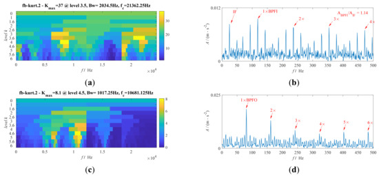
Figure 10.
Results by FK for the signals from MFPT: (a,b) correspond to the kurtogram and SES of the inner race fault bearing; (c,d) correspond to the kurtogram and SES of the outer race fault bearing.
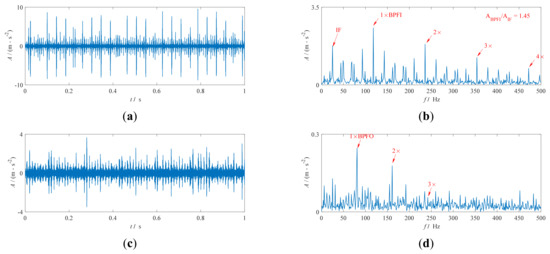
Figure 11.
Results by ICF-VMD for the signals from MFPT: (a,b) correspond to the TDW and SES of the inner race fault bearing; (c,d) correspond to the TDW and SES of the outer race fault bearing.
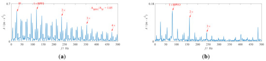
Figure 12.
Results by RVMD with the traditional definition of kurtosis for the signals from MFPT: SES for (a) the inner and (b) outer race fault signals.
3.3. Case II
In the last section, two signals are applied to verify the effectiveness of the proposed method. However, the two signals cannot highlight the whole superiority of RVMD because interference impulses are not included in these two signals. Thus, another signal that includes some large interference impulses is applied to show the superiority of our method.
The signal comes from the Curtin University [34]. The type of test bearing is MB ER-16K, and a local defect exists in its outer race. This signal is marked as CU-O in this study for convenience. The shaft speed is 1740 rpm, and the BPFO is 103.6 Hz. The sampling frequency is 51.2 kHz, and the signal length applied in this study is 1 s. The TDW and SES of the raw signal are shown in Figure 13. Some large interference impulses (marked by red points) are included in the measured signal, as shown in Figure 13a. The fault feature frequency and its harmonics are difficult to observe in the SES shown in Figure 13b. Then, the proposed method is applied to analyze this signal, and the results are shown in Figure 14. From it, the second sub-mode should be analyzed by envelope analysis technology to show the fault feature. The responding result is shown in Figure 15. The fundamental fault feature frequency and its harmonics are clearly shown in it, indicating that the proposed method has succeeded in extracting the bearing fault feature from the signal polluted by some large impulses.
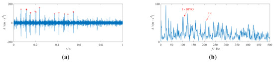
Figure 13.
The signal from Curtin University: (a) TDW and (b) SES.
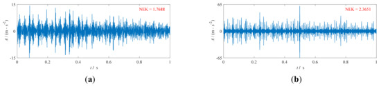
Figure 14.
Results by RVMD for the signal from the Curtin University: (a) the first and (b) second sub-modes.
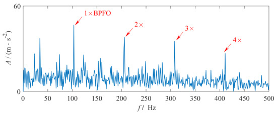
Figure 15.
SES of the results by RVMD for the signal from the Curtin University.
This signal is also processed by FK, ICF-VMD, and RVMD with the traditional EK. The corresponding results are shown in Figure 16, Figure 17 and Figure 18, respectively. From Figure 16a, the ODFB for this signal is in level 3 with the center frequency of 8000 Hz. The corresponding SES is shown in Figure 16b, where only the fundamental fault feature frequency can be observed clearly. Figure 17a shows the TDW of the result by ICF-VMD. From it, there are still some large interference impulses in the filtered signal, which means ICF-VMD fails to suppress the interference impulses. Meanwhile, the SES shown in Figure 17b indicates ICF-VMD fails to extract the periodic impulses. Figure 18 displays the result by RVMD with the traditional definition of kurtosis, where the fault features are seriously interfered with due to the existence of noise. By comparing its two sub-modes, shown in Figure 19, we find the reason is that EK with traditional kurtosis fails to identify the sub-mode which includes the periodic impulses. This means the redefined kurtosis in this study can suppress the interferences from large aperiodic impulses effectively. Consequently, we can say our method can accurately extract bearing fault features and has a strong resistance against interference from aperiodic impulses.
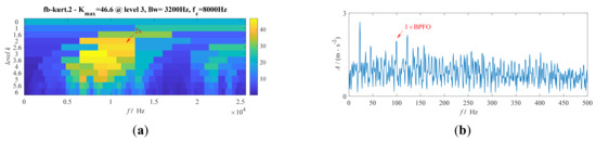
Figure 16.
Results by FK for the signal from the Curtin University: (a) Kurtogram and (b) SES.
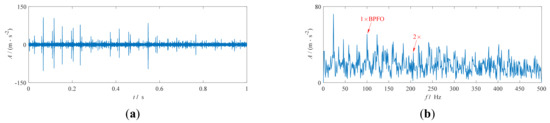
Figure 17.
Results by the ICF-VMD for the signal from the Curtin University: (a) TDW and (b) SES.
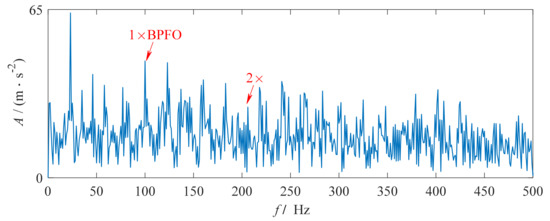
Figure 18.
Result by RVMD with the traditional definition of kurtosis for the signal from the Curtin University.
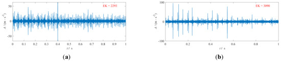
Figure 19.
TDW by RVMD with the EK for the signal from the Curtin University: (a) IMF1 and (b) IMF2.
4. Conclusions
Kurtosis is redefined on the basis of the number of elements whose values are above the RSM of the squared data to enhance its anti-interference ability. The ensemble kurtosis based on the redefined kurtosis works well to evaluate the ratio of the periodic impulses to the noisy signal. By combining the new ensemble kurtosis with VMD, RVMD is designed as two stages to adaptively extract the periodic impulses for bearing fault diagnosis. The effectiveness of RVMD is verified by the simulation signal and bearing fault signals. The advantage of RVMD is presented by comparing it with some other existing methods. Overall, the results in this study greatly contribute to bearing fault diagnosis.
Author Contributions
Funding acquisition, Y.L., Y.C.; project administration, Y.L., Y.C.; conceptualization, Y.L., B.L.; validation, Y.L.; formal analysis, Y.L., B.L.; investigation, Y.L., Y.W.; data curation, B.L., Y.W.; writing—original draft preparation, Y.L.; writing—review and editing, Y.L. All authors have read and agreed to the published version of the manuscript.
Funding
This work was supported by the National Natural Science Foundation of China (Grant Nos. 61633005).
Institutional Review Board Statement
Not applicable.
Informed Consent Statement
Not applicable.
Data Availability Statement
Not applicable.
Conflicts of Interest
The authors declare no conflict of interest.
References
- He, B.; Huang, Y.; Wang, D.; Yan, B.; Dong, D. A parameter-adaptive stochastic resonance based on whale optimization algorithm for weak signal detection for rotating machinery. Meas. J. Int. Meas. Confed. 2019, 136, 658–667. [Google Scholar] [CrossRef]
- Akay, B.; Ragni, D.; Ferreira, C.S.; Van Bussel, G. Experimental investigation of the root flow in a horizontal axis wind turbine. Wind. Energy 2014, 17, 1093–1109. [Google Scholar] [CrossRef]
- Zhan, Y.; Tan, Q.; Zhang, Y. The Application of Morphology Analysis and BTFSVM to Intelligent Fault Diagnosis on the Bearing of Ships. In 2009 Second International Symposium on Knowledge Acquisition and Modeling; IEEE Computer Society: Washington, DC, USA, 2009; Volume 3, pp. 233–236. [Google Scholar] [CrossRef]
- Xing, Z.; Lin, J.; Huang, Y.; Yi, C. A Feature Extraction Method of Wheelset-Bearing Fault Based on Wavelet Sparse Representation with Adaptive Local Iterative Filtering. Shock Vib. 2020, 2020. [Google Scholar] [CrossRef]
- Yu, J.; Hu, T.; Liu, H. A New Morphological Filter for Fault Feature Extraction of Vibration Signals. IEEE Access 2019, 7, 53743–53753. [Google Scholar] [CrossRef]
- Dolenc, B.; Boškoski, P.; Juričić, Đ. Distributed bearing fault diagnosis based on vibration analysis. Mech. Syst. Signal Process. 2016, 66–67, 521–532. [Google Scholar] [CrossRef]
- Zhang, H.; He, Q. Tacholess bearing fault detection based on adaptive impulse extraction in the time domain under fluctuant speed. Meas. Sci. Technol. 2020, 31, 074004. [Google Scholar] [CrossRef]
- Cui, L.; Wang, J.; Lee, S. Matching pursuit of an adaptive impulse dictionary for bearing fault diagnosis. J. Sound Vib. 2014, 333, 2840–2862. [Google Scholar] [CrossRef]
- Zhuang, Z.; Ding, J.; Tan, A.C.; Shi, Y.; Lin, J. Fault Detection of High-Speed Train Wheelset Bearing Based on Impulse-Envelope Manifold. Shock. Vib. 2017, 2017, 1–17. [Google Scholar] [CrossRef]
- Lv, Y.; Zhu, Q.; Yuan, R. Fault Diagnosis of Rolling Bearing Based on Fast Nonlocal Means and Envelop Spectrum. Sensors 2015, 15, 1182–1198. [Google Scholar] [CrossRef] [PubMed]
- Huang, N.E.; Shen, Z.; Long, S.R.; Wu, M.C.; Shih, H.H.; Zheng, Q.; Yen, N.-C.; Tung, C.C.; Liu, H.H. The empirical mode decomposition and the Hilbert spectrum for nonlinear and non-stationary time series analysis. Proc. R. Soc. A Math. Phys. Eng. Sci. 1998, 454, 903–995. [Google Scholar] [CrossRef]
- Lei, Y.; Lin, J.; He, Z.; Zuo, M.J. A review on empirical mode decomposition in fault diagnosis of rotating machinery. Mech. Syst. Signal Process. 2013, 35, 108–126. [Google Scholar] [CrossRef]
- Chen, J.; Li, Z.; Pan, J.; Chen, G.; Zi, Y.; Yuan, J.; Chen, B.; He, Z. Wavelet transform based on inner product in fault diagnosis of rotating machinery: A review. Mech. Syst. Signal Process. 2016, 70–71, 1–35. [Google Scholar] [CrossRef]
- Cao, H.; Fan, F.; Zhou, K.; He, Z. Wheel-bearing fault diagnosis of trains using empirical wavelet transform. Meas. J. Int. Meas. Confed. 2016, 82, 439–449. [Google Scholar] [CrossRef]
- Kedadouche, M.; Thomas, M.; Tahan, A. A comparative study between Empirical Wavelet Transforms and Empirical Mode Decomposition Methods: Application to bearing defect diagnosis. Mech. Syst. Signal Process. 2016, 81, 88–107. [Google Scholar] [CrossRef]
- Zhang, X.; Liang, Y.; Zhou, J.; Zang, Y. A novel bearing fault diagnosis model integrated permutation entropy, ensemble empirical mode decomposition and optimized SVM. Meas. J. Int. Meas. Confed. 2015, 69, 164–179. [Google Scholar] [CrossRef]
- Yan, R.; Gao, R.X.; Chen, X. Wavelets for fault diagnosis of rotary machines: A review with applications. Signal Process. 2014, 96, 1–15. [Google Scholar] [CrossRef]
- Dragomiretskiy, K.; Zosso, D. Variational Mode Decomposition. IEEE Trans. Signal Process. 2014, 62, 531–544. [Google Scholar] [CrossRef]
- Wang, Y.; Markert, R. Filter bank property of variational mode decomposition and its applications. Signal Process. 2016, 120, 509–521. [Google Scholar] [CrossRef]
- Wang, Y.; Markert, R.; Xiang, J.; Zheng, W. Research on variational mode decomposition and its application in detecting rub-impact fault of the rotor system. Mech. Syst. Signal Process. 2015, 60–61, 243–251. [Google Scholar] [CrossRef]
- Li, Z.; Jiang, Y.; Guo, Q.; Hu, C.; Peng, Z. Multi-dimensional variational mode decomposition for bearing-crack detection in wind turbines with large driving-speed variations. Renew. Energy 2018, 116, 55–73. [Google Scholar] [CrossRef]
- Li, F.; Li, R.; Tian, L.; Chen, L.; Liu, J. Data-driven time-frequency analysis method based on variational mode decomposition and its application to gear fault diagnosis in variable working conditions. Mech. Syst. Signal Process. 2019, 116, 462–479. [Google Scholar] [CrossRef]
- Li, Y.; Li, G.; Wei, Y.; Liu, B.; Liang, X. Health condition identification of planetary gearboxes based on variational mode decomposition and generalized composite multi-scale symbolic dynamic entropy. ISA Trans. 2018, 81, 329–341. [Google Scholar] [CrossRef] [PubMed]
- Huang, Y.; Lin, J.; Liu, Z.; Wu, W. A modified scale-space guiding variational mode decomposition for high-speed railway bearing fault diagnosis. J. Sound Vib. 2019, 444, 216–234. [Google Scholar] [CrossRef]
- Xu, B.; Zhou, F.; Li, H.; Yan, B.; Liu, Y. Early fault feature extraction of bearings based on Teager energy operator and optimal VMD. ISA Trans. 2019, 86, 249–265. [Google Scholar] [CrossRef]
- Zhang, X.; Miao, Q.; Zhang, H.; Wang, L. A parameter-adaptive VMD method based on grasshopper optimization algorithm to analyze vibration signals from rotating machinery. Mech. Syst. Signal Process. 2018, 108, 58–72. [Google Scholar] [CrossRef]
- Miao, Y.; Zhao, M.; Lin, J. Identification of mechanical compound-fault based on the improved parameter-adaptive variational mode decomposition. ISA Trans. 2019, 84, 82–95. [Google Scholar] [CrossRef]
- Li, Z.; Chen, J.; Zi, Y.; Pan, J. Independence-oriented VMD to identify fault feature for wheel set bearing fault diagnosis of high speed locomotive. Mech. Syst. Signal Process. 2017, 85, 512–529. [Google Scholar] [CrossRef]
- Jiang, X.; Shen, C.; Shi, J.; Zhu, Z. Initial center frequency-guided VMD for fault diagnosis of rotating machines. J. Sound Vib. 2018, 435, 36–55. [Google Scholar] [CrossRef]
- Lian, J.; Liu, Z.; Wang, H.; Dong, X. Adaptive variational mode decomposition method for signal processing based on mode characteristic. Mech. Syst. Signal Process. 2018, 107, 53–77. [Google Scholar] [CrossRef]
- Gong, T.; Yuan, X.; Yuan, Y.; Lei, X.; Wang, X. Application of tentative variational mode decomposition in fault feature detection of rolling element bearing. Meas. J. Int. Meas. Confed. 2019, 135, 481–492. [Google Scholar] [CrossRef]
- Jiang, X.; Wang, J.; Shi, J.; Shen, C.; Huang, W.; Zhu, Z. A coarse-to-fine decomposing strategy of VMD for extraction of weak repetitive transients in fault diagnosis of rotating machines. Mech. Syst. Signal Process. 2019, 116, 668–692. [Google Scholar] [CrossRef]
- Available online: https://www.mfpt.org/fault-data-sets/ (accessed on 2 June 2020).
- Available online: https://github.com/sli1989/dataset/tree/master/bearing/inner_outer_race_bearing_fault (accessed on 3 June 2020).
Publisher’s Note: MDPI stays neutral with regard to jurisdictional claims in published maps and institutional affiliations. |
© 2021 by the authors. Licensee MDPI, Basel, Switzerland. This article is an open access article distributed under the terms and conditions of the Creative Commons Attribution (CC BY) license (http://creativecommons.org/licenses/by/4.0/).