Abstract
In this study, vibration based non-destructive testing (NDT) technique is adopted for assessing the condition of in-service timber pole. Timber is a natural material, and hence the captured broadband signal (induced from impact using modal hammer) is greatly affected by the uncertainty on wood properties, structure, and environment. Therefore, advanced signal processing technique is essential in order to extract features associated with the health condition of timber poles. In this study, Hilbert–Huang Transform (HHT) and Wavelet Packet Transform (WPT) are implemented to conduct time-frequency analysis on the acquired signal related to three in-service poles and three unserviceable poles. Firstly, mother wavelet is selected for WPT using maximum energy to Shannon entropy ratio. Then, the raw signal is divided into different frequency bands using WPT, followed by reconstructing the signal using wavelet coefficients in the dominant frequency bands. The reconstructed signal is then further decomposed into mono-component signals by Empirical Mode Decomposition (EMD), known as Intrinsic Mode Function (IMF). Dominant IMFs are selected using correlation coefficient method and instantaneous frequencies of those dominant IMFs are generated using HHT. Finally, the anomalies in the instantaneous frequency plots are efficiently utilised to determine vital features related to pole condition. The results of the study showed that HHT with WPT as pre-processor has a great potential for the condition assessment of utility timber poles.
1. Introduction
Timber is a commonly used industrial material due to its accessibility and wide variety of mechanical and physical properties, such as higher strength to weight ratio, electrical, and heat insulation and having a simpler and faster installation process [1]. Timber poles are broadly used worldwide since they are environmental friendly and significantly cheaper than other alternative materials [1]. Currently, more than 5 million utility timber poles are used in Australia’s infrastructure which represent 80% of the total poles [2]. Approximately 70% of these timber poles were installed before 1965 [3]. They will require maintenance and need replacement soon and related cost may reach up to AU$1.75 billion [3]. Routine inspections are carried out on a regular basis to monitor pole condition which deteriorates over time due to fungal and termite attacks and climate and soil condition. For maintenance and asset management, utility pole industry spends AU$50 million yearly to avoid pole failure and ensure reliability of energy network [3]. In addition, the current pole assessment techniques available in the market mainly rely on visual inspection, sounding, and drilling. However, first two techniques greatly depend on the skill of an asset inspector, which cannot provide consistent accuracy required for ensuring public safety, and drilling is commonly conducted at the ground level reflecting the local condition of the pole. However, damage can present in underground section or top part of the pole which is unreachable by the asset inspector and that often results into inaccurate prediction of the health state. Advanced methods like X-ray, ultrasonic tomography, and radiographic methods use cross-sectional evaluation and can yield highly accurate results. Nevertheless, access to the underground or overhead information remain a challenge. Additionally, use of these methods are limited due to high cost, limited computational efficiency, and complexity in the operation [4]. To overcome these limitations, variety of non-destructive testing (NDT) methods have been investigated and developed by the engineers and researchers in the past two decades to provide accurate information on the condition of timber pole/pile structures such as wave based, and vibration based, NDT methods.
In case of vibration based method, timber pole is hit manually by a modal hammer and a broadband low frequency input signal is generated [5]. Because the input frequency is low, generated signal has long wavelength. When the wavelength of the signal gets bigger than the diameter of the pole, the induced stress wave creates a standing wave within the pole resulting into vibration of the whole pole [6]. Vibration based method has been utilised for non-destructive evaluation of timber poles to assess the underground and top part of the pole since it has higher propagating energies. This method has been successfully used by many researchers for timber poles [7,8,9,10,11], tree logs [12,13,14], and pile type structures [15,16]. Table 1 demonstrates comparison of the reviewed NDT methods for this study.

Table 1.
Comparison of the reviewed non-destructive testing (NDT) methods for this study.
In this paper, vibration based method is adopted in order to investigate the condition of utility timber poles since this method can analyse the whole pole by utilizing its dynamic properties such as natural frequency, mode shapes, damping ratio [17]. Natural frequency is the most popular damage indicator in the early years of vibration-based damage detection as it is easy to determine and is generally less affected by ambient noise [18,19,20,21,22]. Natural frequency-based methods depend on the fact that damage in a structure reduces the structural stiffness which actually changes the resonance frequencies. Nonetheless, these methods are model based and need a mathematical model of the structure to obtain vibration frequencies. Another shortcoming is that changes in frequency caused by cracks is not very prominent and is often buried under operational and environmental conditions. Despite some successful application of using natural frequencies as a feature for vibration-based NDT, extensive research proved that natural frequency alone is a poor indicator of damage for the condition assessment due to its low sensitivity to damage especially when severity is low. Hu and Afzal [10] determined the first two natural frequencies of six damaged timber beams and compared against the same of the intact ones. Their results showed that first natural frequency is not appropriate for identifying low-level damage.
Numerous researchers proposed that mode shapes and their derivatives are more consistent and better indicator than natural frequencies as they have local information that makes them capable to detect multiple cracks. Moreover, they are less effected by environmental change, for instance, temperature [23]. However, limitations exist in mode shape-based methods. Firstly, a dense array of sensors is required to obtain mode shapes and secondly, they are more susceptible to noise compared to the natural frequencies. Features that utilise natural frequencies and mode shapes together [24], or derivatives of mode shapes; for example, mode shape curvature [25], modal flexibility [26], modal strain energy [27,28] are found to be effective for damage identification. Samali et al. [10] proposed a modified damage index method for locating damage in timber beams by utilising first five mode shapes of the structure and their derivatives attained from the experimental modal analysis. According to the researchers, the modified algorithm is reliable and economical with few anomalies. Hu and Afzal [23] used a damage indicator derived from the difference between mode shapes with and without damage using discrete Laplace transform for detecting multiple damage in timber beams. The damage indicator was sensitive for designed damage scenarios. However, it was unable to assess the severity of damage quantitatively. Moreover, the method was also computationally and economically expensive, since it required 43 impact points for each set of data in the modal tests. Peterson et al. [29,30] adopted a damage index method for a one-dimensional (1-D) system that utilises modal strain energy to detect local damage and decay in timber beams using first two flexural modes. The proposed method found to be effective for single damage scenarios. However, it yielded limited accuracy for the multi damage scenarios.
Nevertheless, these dynamic properties are affected by orthotropic behaviour of timber material, various species of wood used for utility poles, changing length and diameter of poles through the distribution network, difference in climate and soil condition, and presence of additional restraints, transformers, cross-arm, and conductors. Furthermore, environmental factors including temperature and moisture content result in difference of material properties even for the same timber species and geometric location. Additionally, the testing data obtained from practical field are often non-stationary and non-linear since the patterns of acquired data frequently changes with time which means frequency components also changes over time. Consequently, pole assessment results vary ominously from the practical condition of tested poles.
Regarding this problem, advanced signal processing techniques play a significant role in the condition assessment of timber poles. The conventional Fourier transform can be effective; however, it transforms the data from time to frequency domain resulting into complete loss of time information. Due to this deficiency, time–frequency analysis has attracted numerous researchers for analyzing field tested broadband signal. Among all the time frequency analysis techniques, Wavelet Transform (WT) and Wavelet Packet Transform (WPT) are widely adopted by researchers to deal with such signals which yielded acceptable outcomes [8,11,31]. In this technique, original broadband signal was first decomposed into several narrow band signals and then the reconstructed signal was obtained for each band using WT or WPT from which features can be extracted. Usually, resolution and decomposition capability is better for WPT than that of WT while considering a discrete signal [31]. WT can only be used for decomposing the original signal in low frequency components, whereas WPT can decompose the same signal in both low and high frequency components. As a result, WPT can process a signal in more details than WT [31]. However, selection of proper mother wavelet is crucial for both WT and WPT. Features that are extracted in vibration based method using signal processing techniques include resonance frequency [7], power spectral density [32], continuous wavelet transform coefficient [8,9], short kernel coefficient [9] and auto-regressive coefficient, energy value, and energy coefficient [11]. The signal processing techniques that are used includes fast Fourier transform [7], continuous wavelet transform [9], short kernel method [9], wavelet packet transform [11], empirical mode decomposition [11], and auto-regressive models [11] in order to extract the above mentioned features. However, these features solely cannot distinguish between serviceable and unserviceable condition poles.
Recently, another time–frequency analysis method named Hilbert–Huang Transform (HHT) has become more popular for analyzing nonstationary and nonlinear signals [33]. HHT has been adopted for the condition assessment of timber poles using stress wave propagation technique with satisfactory results [34,35]. The key part of HHT is empirical mode decomposition (EMD) that can decompose field captured broadband signals into subcomponents or mono-component signals denoted as intrinsic mode function (IMFs). Later, Hilbert transform is applied to those IMFs to obtain instantaneous amplitude and instantaneous frequency, thus Hilbert spectrum can be derived representing full energy–time–frequency distribution. EMD process does not require any convolution [36]. Compared to the Wavelet transform, the computation time for EMD is also less.
Moreover, it is noteworthy to mention that the concept of the frequency and time resolution is not included in HHT [37]. Instantaneous frequency obtained from HHT has a meaning only for mono-component signals and signals obtained from field are not mono-component but multicomponent. Hilbert transform of IMFs (generated from EMD process) lead to physically meaningful instantaneous frequencies. However, in practice, HHT suffers from a number of deficiencies. First of all, the EMD process generates some unwanted IMFs in the low frequency range that can be misleading during data interpretation of the data [36]. Secondly, depending on the analysed signal, the first IMF may cover broad range of frequency in the high frequency range as well which cannot satisfy the mono component property of IMF [36].
Accordingly, WPT and HHT are employed together in this paper to overcome the aforementioned challenges. This technique is employed on signals associated with three serviceable and three unserviceable timber poles. Selection of mother wavelet is important for the WPT. Maximum energy to Shannon entropy ratio is adopted to select the best mother wavelet function. Using WPT, the captured vibration signal is decomposed into different frequency bands and wavelet coefficients are reconstructed in the dominant frequency bands as new signal for performing further decomposition using EMD. Furthermore, a screening technique is applied to select the dominant IMFs produced from EMD to eliminate the undesirable IMFs by computing the correlation coefficients of the IMFs and the raw analysed signal. Later, Hilbert Transform is applied to those dominant IMFs in order to generate the instantaneous frequency plot.
The effectiveness of the improved HHT is verified for six poles data collected from real field. Sudden changes in the instantaneous frequencies are observed in the analysed signal to determine some vital features related to the health state of timber pole. HHT with the WPT as pre-processor has been successfully used by Z. Peng et al. [36,37] for roller bearing fault diagnosis, nevertheless there is still no report on the implementation of this technique in vibration based damage detection of utility timber poles.
2. Limitation of Original Hilbert Huang Transform:
2.1. Hilbert–Huang Transform
Huang et al. [38] first introduced Hilbert–Huang transform(HHT) as an adaptive method for analysing nonstationary and nonlinear signals in 1998. Hilbert transform of an arbitrary signal has the local properties of is well-defined as the convolution of the signal with as follows:
where is the Cauchy principal value. Analytical signal of can be found through coupling and , as
where is the instantaneous amplitude of , which can reflect how the energy of the signal changes with time, and is the instantaneous phase of . Main property of Hilbert Transform is the instantaneous frequency which has a meaning only for mono-component signals. It can be defined as the presence of only one frequency value at a given time frame or signal. The physical meaning of instantaneous frequency of a signal can be found from the time derivative of instantaneous phase as the following:
However, practical signals obtained from the field are complex and contains more than one frequency component at a time. In order to obtain physically meaningful instantaneous frequencies, original signal captured from field should have one frequency or a narrow band of frequencies that vary as a function of time. Therefore, captured complex multicomponent signal must be divided into subcomponents. Huang et al. [38] proposed a new decomposition technique called Empirical mode decomposition (EMD) for this purpose. EMD is capable of decomposing a complex multicomponent signal into nearly mono component signals which are referred as intrinsic mode functions (IMFs). These IMFs usually satisfy two conditions:
- The number of extrema and the number of zero crossings should be equal or differ by at most one when considering whole data set.
- The mean value of the envelope defined by the local maxima and local minima is zero at any point.
A given signal can be decomposed into different IMFs through EMD process. At first, all the local maxima and local minima points from a given signal are identified. Using cubic spline method, these points are interpolated into upper and lower envelope of the signal. Secondly, the mean value of upper and lower envelope is calculated which is denoted as , and the difference between the signal and is the first component of shifting process denoted as [38] as follows,
where should satisfy the condition of IMF but ideally that is not the case. is considered as new signal and the whole shifting process is repeated until satisfy the condition of a true IMF, denoted as . Hence, 1st IMF is obtained which is the highest frequency component in the original signal. Later, is removed from rest of the signal and the residue of the signal is obtained which is expressed as follows:
Then this is considered as a new signal and the whole procedure is repeated to find , , , …, and , , , …, . Stopping criteria for the shifting process is also defined by Huang et al. [38] for the standard deviation value which is calculated from two consecutive shifting results and the value is limited between 0.2 and 0.3. Accordingly, the shifting process will be terminated when and meets pre-determined stopping criteria and becomes constant or a monotonic function from which no more IMF can be extracted [38]. The input signal can be reconstructed by adding all the IMFs and final residue .
These IMFs are symmetric, and they will have different frequency at a particular time. Hilbert Transform is then applied to each IMF and instantaneous frequency and amplitude are calculated according to Equations (3) and (5). Now the original signal is expressed as
The EMD process combined with Hilbert transform is known as Hilbert–Huang transform (HHT) and using HHT, original signal can be represented in its instantaneous amplitude, frequency, and time in a three-dimensional plot. Thus, a full energy-frequency-time distribution can be obtained which is known as Hilbert spectrum.
2.2. Limitation of Hilbert–Huang Transform for Multicomponent and Nonstationary Signals
In this section, a multicomponent and nonstationary signal is analysed using the original HHT to discuss its limitation. Figure 1 shows a multicomponent nonstationary signal which is sampled at 2000 Hz for 4 s and contains 50 Hz, 100 Hz, and 200 Hz frequency components. Signal’s frequency is initially 50 Hz and 100 Hz and increases to 200 Hz after 2 s. Figure 2 depicts the signal’s IMFs and the residue obtained through EMD process, whereas Figure 3 demonstrates instantaneous frequencies of those corresponding IMFs produced from HHT. Colour bar in Figure 3 represents instantaneous amplitude of the results. From Figure 2 and Figure 3, it is obvious that IMF1 and IMF2 are the real frequency components that correspond to 200, 100, and 50 Hz, respectively. Moreover, the change in amplitude and frequency from 100 Hz to 200 Hz after 2 s are visible from the Hilbert spectrum plot of IMF1 (Figure 3). Other IMFs in the low frequency region are pseudo-components of the multicomponent signal, which is misleading for the data interpretation.
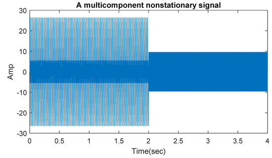
Figure 1.
A multicomponent nonstationary signal.
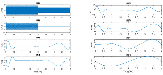
Figure 2.
Intrinsic Mode Functions (IMFs) of the multicomponent nonstationary signal.
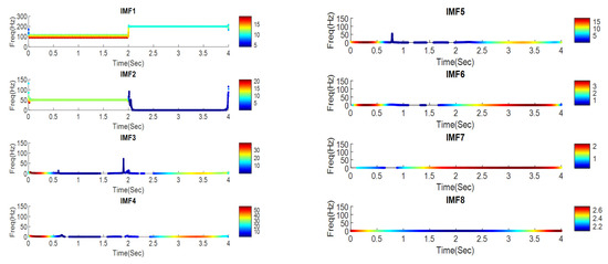
Figure 3.
Instantaneous frequencies of the multicomponent nonstationary signal.
This type of phenomenon occurs due to the cubic spline process inherent in EMD. During cubic spline process, large swings occur at both ends of the signal that can propagate inside the signal. As a result, whole signal gets corrupted, and some undesirable IMFs are produced in the low frequency region. Eventually, these undesirable IMFs may provide misleading information regarding the health state of utility timber poles.
Another shortcoming of HHT is that the first IMF contains a wide range of frequency in the high frequency region in practice [36]. Ideally, IMF should be nearly mono component but in case of IMF1, the mono component property cannot be achieved. Practical signals obtained from field contain more than one frequency at the same time, and IMF will not have one frequency component or narrow range of frequencies. Nevertheless, the instantaneous frequency of IMF1 will be still significant to some extent since IMF1 fulfils the two conditions an IMF should satisfy, and its instantaneous frequency will still be restricted in its own frequency range.
3. Improved Hilbert Huang Transform
3.1. Wavelet Packet Transform
In order to deal with the above-mentioned problem, the inspected signal can be pre-processed into several narrow band signals first and then those narrowband signals can be decomposed by EMD. Therefore, the processed IMF will be in narrow frequency range and their instantaneous frequencies computed using Equation (5) will be in narrow range. There are several methods available to act as a pre-processor for decomposing the original signal into various narrow band signals. In this paper, WPT is adopted as a proper pre-processor due to its computational efficiency and well-recognised properties of being orthogonal, complete, and local [36]. Figure 4 exhibits WPT decomposition tree (three levels) of a time series signal .
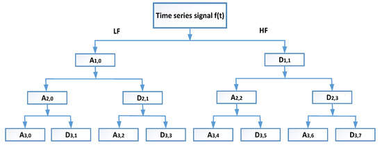
Figure 4.
Wavelet Packet Transform decomposition tree (three levels).
First, the time series signal is passed through couple of low-pass filter (LF) and high-pass filter (HF) in order to divide into low frequency and high frequency components known as approximation coefficient (A1,0) and detail coefficient (D1,1) respectively. The approximation coefficient (A1,0) and the detail coefficient (D1,1) will split themselves again into a second level approximation and detail coefficients and the process is repeated. WPT can be expressed as Equation (10).
where is a wavelet packet function with three indices , , corresponding to modulation, scale, and translation parameters, respectively. Wavelet function is derived from the following recursive equations:
where and are quadrature mirror filters related to the scaling function and mother wavelet function, respectively. Wavelet packet coefficients of signal are calculated using the following expression.
Each wavelet packet component is reconstructed individually to make a part of the signal using inverse wavelet transform. The reconstructed signal from wavelet packet is as follows:
The original raw signal is obtained by summing the reconstructed signals from packets of th level decomposition as follows:
The frequency band of each packet at th level decomposition, is computed as follows:
where is the sampling frequency.
3.2. Mother Wavelet Selection
Selection of proper mother wavelet is vital in WPT since the results obtained from WPT will get affected by the chosen mother wavelet. In this study, maximum energy to Shannon entropy criterion is utilised to select the proper mother wavelet. Rostaghi et al. [39] and Rodrigues et al. [40] used a similar criterion for rotating machinery vibration signal analysis using WPT and DWT. According to this criterion, the mother wavelet that produces the maximum energy to Shannon entropy ratio is selected as the most appropriate one. Energy of the signal is obtained from the following expressions:
where is the energy of th wavelet packet component at th decomposition level of the signal and is the sum of all packet component’s energy in th level. actually represents the energy of original raw signal. Shannon entropy () is defined as follows:
Maximum energy to Shannon entropy criterion, is calculated using Equation (21).
3.3. Dominant IMF Selection Method
A simple but effective screening technique can be applied in order to get rid of the undesirable IMFs in the low frequency region. Since IMFs are nearly an orthogonal demonstration of the original signal, the dominant IMFs will be strongly correlated with the original signal. On contrary, the pseudo-components will have poor correlation with the inspected signal. Based on this concept, correlation coefficients of IMFs and the inspected signal can be utilised to select the dominant IMFs. Using this method, correlation coefficients of the IMFs and the multicomponent nonstationary signal from Figure 1 are calculated and listed in Table 2. From Table 2, it can be observed that only the first two IMFs have strong correlation with the inspected multicomponent signal having large correlation coefficients whilst other IMFs have a very poor correlation with the inspected signal. Moreover, IMF1 and IMF2 actually contain the real frequency components of the inspected multicomponent nonstationary signal.
The proposed combination of HHT and WPT is adopted from the studies of Z. Peng [36,37]. Operation procedures of improved HHT is shown in Figure 5. Experimental program is described in the following section and the effectiveness of improved HHT along with the mother wavelet selection and IMF selection method will be verified in Section 5 through a comparative study between original HHT and improved HHT for serviceable/healthy in situ timber poles.
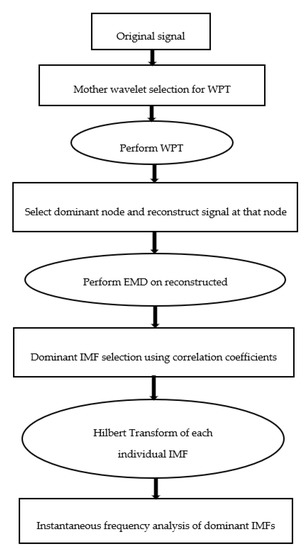
Figure 5.
Operation procedures of proposed Hilbert–Huang Transform (HHT).
4. Experimental Program
4.1. Equipment
To validate the proposed method, vibration testing method using impact hammer was implemented on three serviceable/healthy and three unserviceable/unhealthy in-situ timber poles. Since timber is an orthotropic material, its material properties vary in three different directions: longitudinal, radial, and circumferential. Subhani et al. [41] proposed an appropriate sensor set up for the non-destructive assessment of cylindrical type structures which has been utilised in this study in order to capture the three dimensional behaviour of timber pole. For field testing, an impact hammer, 12 accelerometers and a data acquisition system were employed. Modal hammer Endevco 2303 was used in this study (1 mV/lbf, 5000 lb range) to generate impact, while Instron 46A16 sensors were used for capturing accelerations with sensitivity of 100 mv/g (range ±50 g). The NI cDAQ-9133 (1.33 GHz, 16 GB) from National Instrument was used as the data acquisition system with NI 9232 (3 channel, +/30 V, 102.4 kS/s/channel, 24-Bit, IEPE AI C Series) input modules. A total of 12 accelerometers were used and was connected to the pole by mechanically means (as shown in Figure 6a). Figure 6b depicts the portable device used for the testing.
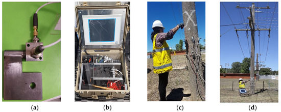
Figure 6.
(a) Accelerometer attachment (b) Pole tester (c) Accelerometer arrangement (d) Field testing.
4.2. Testing Specimen
Field testing is executed on three serviceable and three unserviceable in situ utility timber poles located at Benalla, Victoria. Detail of the testing specimen is given in Table 3 and Table 4.
Table 3.
Detail of three in-situ serviceable timber poles.
Table 4.
Detail of three unserviceable timber poles.
The data related to these 6 were collected on the same day and from the same geographical location, as mentioned in Table 3 and Table 4. Condition of these poles were determined by the asset inspector from Ausnet Services using dig and drill method. Figure 7 demonstrates pole inspection below ground line using dig and drill method. Usually, 300 mm deep excavation is done around the pole. Then, ground inspection holes are drilled to the centre of the pole at an angle of 20 degree between ground line and 150 mm from the ground line (see Figure 7). This method is undertaken in the suspected area in order to allow measurement of internal deterioration and amount of sound wood. If sound wood measurement is below 30 mm, pole is considered as unserviceable, whereas measurement above 50 mm is considered as serviceable; also, measurements between 30 mm and 50 mm are considered as having a limited service life.
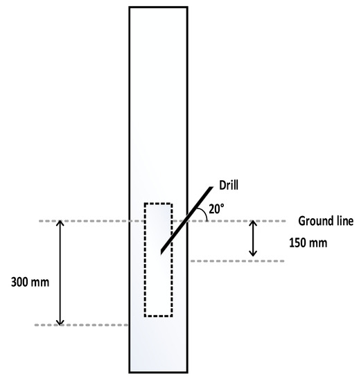
Figure 7.
Pole inspection below ground line using dig and drill method.
4.3. Testing Specimen
Figure 6 and Figure 8 demonstrate the experimental field set up for the vibration testing. Hammer impact was induced at a height of 1500 mm on the side of the pole with an angle of 45°. The sampling frequency was set to 100 kHz. Each pole was struck four times. Accelerometers were attached on the pole at 1200 mm and 900 mm from the ground level. Six accelerometers that are located at 1200 mm from the bottom of the pole are designated as layer 1 accelerometers and the other six accelerometers that are located at 900 mm from the bottom of the pole are designated as layer 2 accelerometers. For each accelerometer location, three positions along the circumference 0°, 90°, and 180° were taken into account. The accelerometer which is aligned with the impact line is named as 0° and the accelerometer opposite to 0° is called 180°. In the same way, the accelerometer which is located 90° around the circumference is called as 90°. Additionally, at each accelerometer position, the displacement was captured in two orthogonal directions, i.e., in the longitudinal (L), radial (R) for 0° and 180° and longitudinal (L) and circumferential (C) for 90°. The illustration of every accelerometer is named such a way that it represents the location and orientation of that particular accelerometer. For instance, a notation “A90C1” means the accelerometer belongs to layer 1 that is located at 1200 mm from the bottom of the pole and the position is 90° around the circumference; also, the displacement component is the circumferential one.
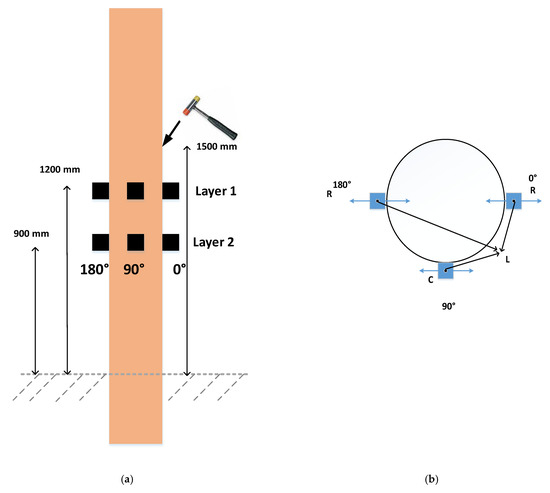
Figure 8.
(a) Schematic diagram of experimental test set up (b) Horizontal cross section.
5. Results and Discussion
5.1. Raw Data
Time domain signal of Serviceable Pole 1 from the hammer impact and its corresponding frequency spectrum after performing Fast Fourier Transform (FFT) are demonstrated in Figure 9a,b, respectively. From the frequency spectrum of impulse, it is observed that the data tends to lose energy when the frequency exceeds 1500 Hz. That means the main frequency range of hammer hit lies between 0 and 1500 Hz. It is also obvious that the low frequency components are dominant in the signal.
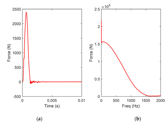
Figure 9.
Hammer impact in (a) time domain (b) frequency spectrum.
Raw acceleration data (time domain) of layer 1 and layer 2 of Pole 1 at 0°, 90°, and 180° position and their corresponding frequency spectrums are shown in Figure 10, Figure 11 and Figure 12, respectively. Frequency response function (FRF) is implemented here to normalise the effect of hammer impact. From the results, it can be observed that the time acceleration signals from all 12 sensors are non-stationary and exhibit nonlinear characteristics. Since all the time information is lost after performing FRF, it is impossible to predict how the frequency components present in the raw acceleration signals and how it changes over time. It is also very difficult to identify which peaks in the frequency spectrum are the dominant frequency.
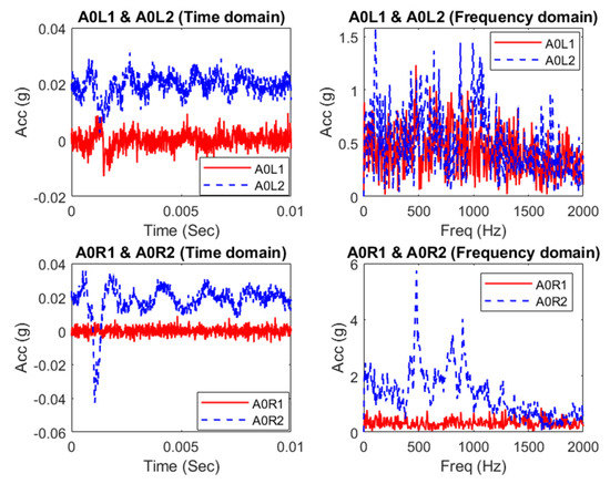
Figure 10.
Captured time domain acceleration data and their frequency spectra at 0° position.
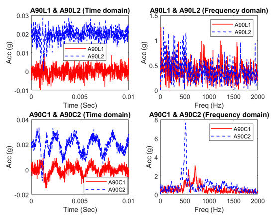
Figure 11.
Captured time domain acceleration data and their frequency spectra at 90° position.
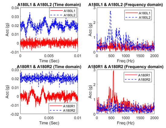
Figure 12.
Captured time domain acceleration data and their frequency spectra at 180° position.
From the comparison of Figure 10 and Figure 12, it can be found that longitudinal components at 0° and 180° position are not in same phase, and they are not out of phase as well. It is also observed that radial components at layer 2 are almost in same phase whereas layer 1 radial components possess very small amplitude. From Figure 11, it can be witnessed that circumferential component is dominant at 90° position and contains more energy than that of longitudinal component at the same position. Behaviour of these three displacement components can be found in details in [41,42].
5.2. Conventional HHT
In this section, acceleration data from A90C1 of Serviceable Pole 1 is analysed using original HHT (using Equation (9)). Figure 13 demonstrates the Hilbert spectrum of the inspected circumferential component generated by original HHT. Colour bars in Figure 13 represent the instantaneous amplitude of the results. Hereinafter, similar colour bar, labels and notations will be used for all Hilbert Spectrums utilised in this study. From this figure, original HHT has produced 13 IMFs after EMD operation. An important observation is that the first five IMFs in the high frequency region contain too wide range of frequency. Consequently, these IMFs can be barely treated as mono-component or nearly mono component signal. It can be noted that most of frequency components present in the first five IMFs are above 2000 Hz which might be related to noise, since the induced frequency was up to 1500 Hz, as shown in Figure 9b. Hence, the original HHT fails to reveal the real frequency pattern of the analysed signal.
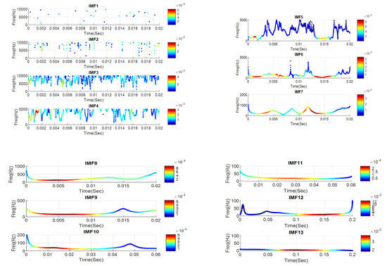
Figure 13.
Instantaneous frequencies of A90C1 Serviceable Pole 1 generated by original HHT.
5.3. Improved HHT
In order to eliminate the high frequency noise components as described in previous section, WPT is employed to decompose the captured acceleration signals into different narrow bands. In addition, selection of mother wavelet function and decomposition level are also described below which are two vital parameters in WPT. In the next section, mother wavelet selection method using maximum energy to Shannon entropy criterion is presented for the acquired acceleration data.
5.3.1. Mother Wavelet Selection
Since discrete wavelet packet is selected for this study, mother wavelet like Meyer, Gaussian, Mexican hat, and other complex wavelets cannot be used [39]. For the analysis, a total 32 mother wavelet functions are considered as shown in Table 5. To select the best mother wavelet, 12 accelerometer data of Serviceable Pole 1 are used in the analysis. First, the dominant wavelet coefficient is obtained based on the maximum energy level. Maximum energy level is found for the first level approximation coefficient (A1,0) for all the accelerometers. Next, the Shannon entropy value is computed for each accelerometer data with respect to each mother wavelet using the dominant wavelet coefficient (A1,0). Energy of the original raw signal from each accelerometer is also calculated. Then the ratio of the energy to Shannon entropy value () is determined for each mother wavelet using Equation (21). Table 6 shows the sample results of 11 mother wavelet functions which have the highest energy to Shannon entropy value among 32 mother wavelets analysed for this study. From the analysis, it is found that bior5.5 wavelet has the maximum ratio of energy to Shannon entropy () and that is why it is chosen as the best mother wavelet for our study.
Table 5.
Mother wavelet functions used in this study.
Table 6.
Results of 11 mother wavelet functions for 12 accelerometers.
5.3.2. Selection of Decomposition Level
In order to select the decomposition levels, it is suitable to select more decomposition levels for reducing the noise interference and extract desirable signal features. However, part of the important local singularities will be lost in the process. Since sampling frequency of 100 kHz gives a signal bandwidth of 50 kHz according to Nyquist sampling theorem, level 5 decomposition level has been selected so that the dominant frequency components between (0 and 1500 Hz) range can fall into node (5,0) of WPT tree. After that, this [5,0] coefficient is reconstructed for all the 12 accelerometers. Frequency band of (5,0) coefficient (0–1562.5 Hz) is considered as the dominant frequency band for our study (based on Figure 8b). An example of reconstructed signal is illustrated in Figure 14. Finally, the reconstructed signals are further decomposed using EMD.
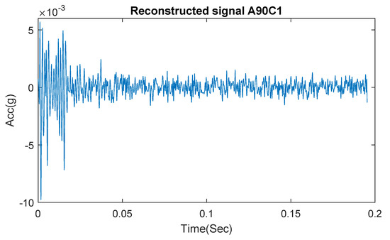
Figure 14.
Example of reconstructed signal considering A90C1 at (5,0) node.
5.3.3. Instantaneous Frequency Analysis Using Improved HHT
In order to overcome the deficiencies of original HHT, improved HHT is employed on the same inspected signal from A90C1 sensor that has been used for analysing original HHT in Section 5.2. First, EMD is performed on the reconstructed signal of A90C1 sensor at (5,0) node from Figure 14. After decomposing this reconstructed signal through EMD, screening technique based on correlation coefficients value is applied to obtain the dominant IMFs. A threshold value of 0.1 is selected for the correlation coefficient in order to avoid accidental removing of some low amplitude but relevant IMFs. After applying improved HHT, 5 dominant IMFs are obtained whereas in case of original HHT applied on the same acceleration data, there were 13 IMFs which can be misleading. Figure 15 demonstrates the dominant IMFs after EMD operation for A90C1. Later, instantaneous frequencies of these dominant IMFs are calculated by Equation (5), and energy–frequency–time distribution of these dominant IMFs, designated as Hilbert spectrum, is shown in Figure 16. In Figure 16, some sharp noisy peaks are observed at both ends of the instantaneous frequency plot. This is known as edge effect which occurs due to the approximation in the EMD process [36]. These sharp peaks at the edges will be avoided for data interpretation.
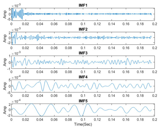
Figure 15.
Dominant IMFs after Empirical Mode Decomposition (EMD) operation for A90C1 Serviceable Pole 1 using improved HHT.
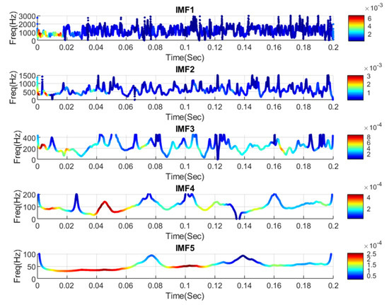
Figure 16.
Instantaneous frequencies of dominant IMFs for A90C1 Serviceable Pole 1 using improved HHT.
One noteworthy behaviour is observed from the Hilbert spectrum of IMF1, A90C1 Serviceable Pole 1. Figure 17 demonstrates the Hilbert spectrum of all IMF1 for A90C1, Serviceable Pole 1 including all 4 tests. From this figure, sudden change and a sharp increase in frequency is observed around 0.02 sec which is very consistent for all the IMF1s. Signal after 0.02 s is related to noise and other uncertainties from field testing. Similar behaviour is noticed for all IMF1s of A90C2 for Serviceable Pole 1 and Serviceable Pole 2 including all four tests. The results look very consistent irrespective of the fact that all these IMF1s have different energy values due to different hammer strikes in each test. Therefore, signal up to 0.02 sec will be considered for data interpretation.
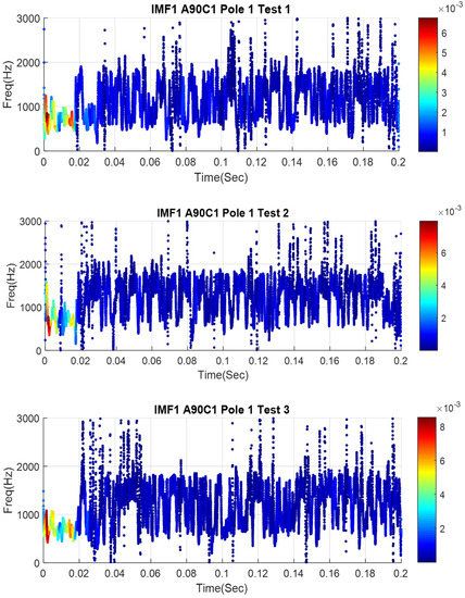
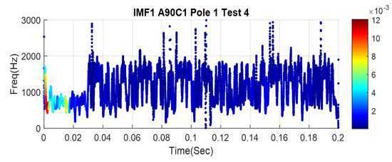
Figure 17.
Hilbert spectrum of IMF1 for A90C1, Serviceable Pole 1 including all 4 tests.
Additional significant finding here is that the improved HHT is able to recover low frequency and low energy components. Considering the signal up to 0.02 sec in Figure 16, it is observed that instantaneous frequency of IMF5 is almost constant at 55 Hz. This is the possible fundamental frequency/natural frequency of that particular pole. Similarly, 105 Hz and 250 Hz frequencies are observed for IMF4 and IMF3, respectively, which are believed to be higher order fundamental frequencies. Since the condition of this pole is believed to be healthy, there are not much sudden changes in the instantaneous frequency of IMF3, IMF4, and IMF5 and very slight changes are observed for IMF2. Similar analysis has been performed for 12 accelerometer data of 3 serviceable poles and 3 unserviceable poles obtained from all 4 tests in order to check the repeatability and consistency of the results. After that, frequency range of dominant IMFs, average frequency of each dominant IMF and standard deviation are calculated. Figure 18 and Figure 19 demonstrate the frequency range of dominant IMFs, average frequency of each dominant IMF and standard deviation for Serviceable Pole 1 and Unserviceable Pole 3, respectively, considering all the accelerometer data. Both the poles are from same species and their strength class and durability class are also same. Frequency range of dominant IMFs for Serviceable Pole 1 are found to be in a similar range with good consistency considering the variability and uncertainty can exist in any field testing (Figure 18). On the other hand, frequency ranges of dominant IMFs for the Unserviceable Pole 3 (from Figure 19) are found to be bigger than that of the serviceable pole case. Standard deviation values are also relatively high for the Unserviceable Pole 3.
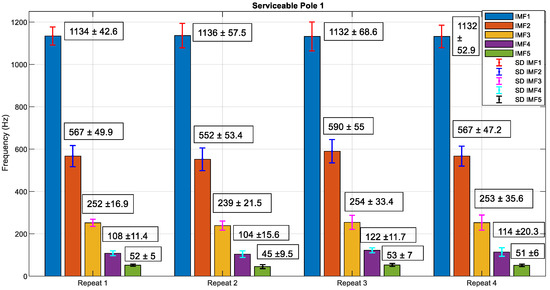
Figure 18.
Bar chart showing frequency range of dominant IMFs, average frequency of each IMF and standard deviation for 12 accelerometers, Serviceable Pole 1.
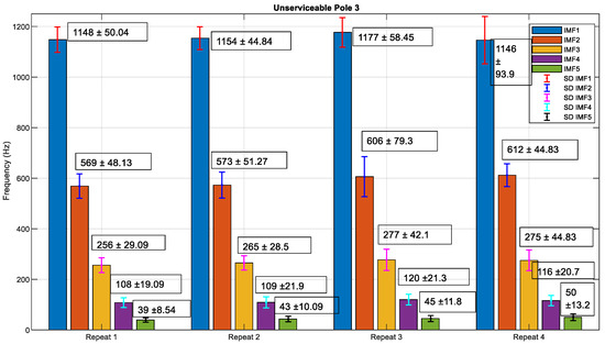
Figure 19.
Bar chart showing frequency range of dominant IMFs, average frequency of each IMF and standard deviation for 12 accelerometers, Unserviceable Pole 3.
Figure 20 shows the instantaneous frequencies of dominant IMFs for A0R2 sensor, Unserviceable Pole 1 using improved HHT. IMF1, IMF2, and IMF3 are found to be dominant for A0R2 sensor using correlation coefficient method. Another major finding from this figure is that instantaneous amplitude of IMF1 is significantly higher than instantaneous amplitude of IMF1 for the serviceable pole case from Figure 16. This phenomenon is observed for sensors in the radial directions which contains highest energy since the hammer impact was made in the radial direction (horizontal). Similarly, instantaneous amplitude of IMF1 for A0R2 are studied for all three serviceable poles and three unserviceable poles.
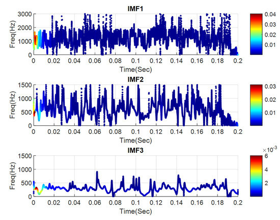
Figure 20.
Instantaneous frequencies of dominant IMFs for A0R2 Unserviceable Pole 3 using improved HHT.
Figure 21 illustrates the instantaneous amplitude of IMF1 for A0R2 considering all six poles used in this study. From this figure, it is clearly observed that instantaneous amplitudes of three unserviceable poles for A0R2 sensor are significantly higher than that of three serviceable poles. This finding is observed for all six poles and for all four repeats which reassures the accuracy and consistency of the study. Figure 22 shows the instantaneous amplitude of IMF1 for A0R1 considering all six poles. From this figure, it is apparent that A0R1 yield the same conclusion (as for A0R2) on considering instantaneous amplitude as damage sensitive feature. However, A0R1 for Unserviceable Pole 1 does not follow this trend. This is related to an error in capturing data during the field testing. To further elaborate this, Figure 23 shows the time vs. acceleration data and their frequency spectrum from A0R1 of Unserviceable Pole 1. From this figure, it is observed that amplitude of A0R1 is very low compared to A0R2 due to connection problem during field testing. As a result, A0R1 did not capture any data while testing Unserviceable Pole 1.
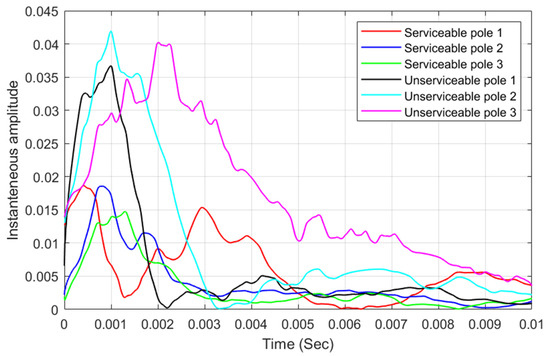
Figure 21.
Instantaneous amplitude of IMF1 for A0R2 considering 3 serviceable poles and 3 unserviceable poles.
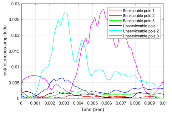
Figure 22.
Instantaneous amplitude of IMF1 for A0R1 considering 3 serviceable poles and 3 unserviceable poles.
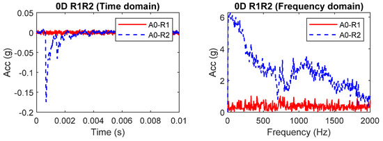
Figure 23.
Captured time domain acceleration data and their frequency spectra at A0R1 and A0R2 for Unserviceable Pole 1.
For this study, instantaneous amplitude of 0.02 obtained from IMF1 of A0R1 and A0R2 (from Figure 21 and Figure 22) is considered as the threshold point to differentiate unserviceable poles from serviceable ones. This observation was consistent for all four repeats as well. Therefore, it can be concluded that instantaneous amplitude will increase according to the severity of damage. If instantaneous amplitude of dominant IMFs is noticed to be increased significantly over time during routine inspection, pole condition can be considered to worsen, and adequate steps should be taken in order to avoid pole failure. Such a finding is vital for condition assessment utility timber poles.
6. Conclusions
In this study, vibration-based NDT using HHT with WPT as pre-processor are adopted for determining features (natural frequencies) of timber poles with a view to assess its condition. In the proposed method, raw vibration signals are captured from field using impact hammer and portable data acquisition system equipped with 12 accelerometers. The signals are multicomponent and nonstationary and use of FRF alone cannot satisfactorily determine the natural frequencies. Therefore, WPT along with a mother wavelet selection method is employed as a pre-processor to decompose the captured raw signal into several narrow bands. Then EMD is utilised on these narrow band signals to obtain IMFs. After that, a simple screening technique is applied to retain the relevant IMFs that are related to the raw signal. Both original HHT and improved HHT have been used to analyse the vibration data of serviceable/healthy and unserviceable/unhealthy in situ timber poles. From the analysis, it is found that improved HHT has better computational efficiency than the original one for the vibration data analysis of timber utility poles. Natural frequencies have been identified which is vital for the health state determination of timber poles. Additionally, condition of the pole can be considered healthy if slight variation in instantaneous frequency is observed for dominant IMFs. From the comparison between serviceable and unserviceable pole, it is found that instantaneous amplitude of dominant IMFs rises according to the severity of damage. Since the condition of the pole vary with time, routine inspection is essential. If amplitude of instantaneous frequency and variations are increased with time, pole condition is referred to have deteriorated and sufficient measures should be undertaken accordingly.
Author Contributions
Conceptualization, M.S.; methodology, I.D. and M.S.; validation, M.S., M.T.A. and I.D.; formal analysis, I.D.; investigation, M.S. and I.D.; funding, A.M.T.O. and M.S.; writing—original draft preparation, I.D.; writing—review and editing, M.S. and M.T.A.; supervision, M.S., M.T.A. and A.M.T.O.; project administration, A.M.T.O. and M.S.; funding acquisition, A.M.T.O. All authors have read and agreed to the published version of the manuscript.
Funding
The research was funded by Ausnet Services, Victoria, Australia.
Institutional Review Board Statement
Not applicable.
Informed Consent Statement
Not applicable.
Acknowledgments
The authors gratefully acknowledge Raj Dassenaike and Steve Clark from Ausnet Services for helping with the data collection of in-service poles. Authors would also like to express their gratitude to James Lamont and Michael Shanahan their supports on packaging the device.
Conflicts of Interest
The authors declare no conflict of interest.
References
- Li, J.; Dackermann, U.; Subhani, M. R&D of NDTs for timber utility poles in service-challenges and applications (extension for bridge sub-structures and wharf structures). In Proceedings of the Workshop on Civil Structural Health Monitoring (CSHM-4), Bundesanstalt für Materialforschung und-prüfung (BAM), Berlin, Germany, 6–8 November 2012. [Google Scholar]
- Nguyen, M.; Foliente, G.; Wang, X.M. State-of-the-practice & challenges in non-destructive evaluation of utility poles in service. Key Eng. Mater. 2004, 270–273, 1521–1528. [Google Scholar] [CrossRef]
- Francis, L.; Norton, J. Australian Timber Pole Resources for Energy Networks. A Review; Technical Report; Department of Primary Industries and Fisheries: Brisbane, Australia, 2006.
- Tanasoiu, V.; Miclea, C.; Tanasoiu, C. Nondestructive testing techniques and piezoelectric ultrasonics transducers for wood and built in wooden structures. J. Optoelectron. Adv. Mater. 2002, 4, 949–957. [Google Scholar]
- Doyle, J.F. Wave propagation in structures. In Wave Propagation in Structures; Springer: New York, NY, USA, 1989; pp. 126–156. [Google Scholar]
- Legg, M.; Bradley, S. Measurement of stiffness of standing trees and felled logs using acoustics: A review. J. Acoust. Soc. Am. 2016, 139, 588–604. [Google Scholar] [CrossRef] [PubMed]
- Krause, M.; Dackermann, U.; Li, J. Elastic wave modes for the assessment of structural timber: Ultrasonic echo for building elements and guided waves for pole and pile structures. J. Civ. Struct. Health Monit. 2015, 5, 221–249. [Google Scholar] [CrossRef]
- Li, J.; Subhani, M.; Samali, B. Determination of embedment depth of timber poles and piles using wavelet transform. Adv. Struct. Eng. 2012, 15, 759–770. [Google Scholar] [CrossRef]
- Subhani, M.; Li, J.; Samali, B.; Yan, N. Determination of the embedded lengths of electricity timber poles utilising flexural wave generated from impactí. Aust. J. Struct. Eng. 2013, 14, 85–96. [Google Scholar] [CrossRef]
- Samali, B.; Li, J.; Dackermann, U.; Choi, F.C. Vibration-based damage detection for timber structures in Australia. In Structural Health Monitoring in Australia; Nova Science Publishers Inc.: Hauppauge, NY, USA, 2011. [Google Scholar]
- Yu, Y.; Dackermann, U.; Li, J.; Subhani, M. Condition assessment of timber utility poles based on a hierarchical data fusion model. J. Comput. Civ. Eng. 2016, 30, 04016010. [Google Scholar] [CrossRef]
- Amishev, D.; Murphy, G.E. Implementing resonance-based acoustic technology on mechanical harvesters/processors for real-time wood stiffness assessment: Opportunities and considerations. Int. J. For. Eng. 2008, 19, 48–56. [Google Scholar] [CrossRef]
- Lindström, H.; Harris, P.; Nakada, R. Methods for measuring stiffness of young trees. Holz als Roh Werkst. 2002, 60, 165–174. [Google Scholar] [CrossRef]
- Lindström, H.; Harris, P.; Sorensson, C.T.; Evans, R. Stiffness and wood variation of 3-year old Pinus radiata clones. Wood Sci. Technol. 2004, 38, 579–597. [Google Scholar] [CrossRef]
- Finno, R.J.; Popovics, J.S.; Hanifah, A.A.; Kath, W.L.; Chao, H.C.; Hu, Y.H. Guided wave interpretation of surface reflection techniques for deep foundations. Ital. Geotech. J. 2001, 36, 76–91. [Google Scholar]
- Lo, K.-F.; Ni, S.-H.; Huang, Y.-H. Non-destructive test for pile beneath bridge in the time, frequency, and time-frequency domains using transient loading. Nonlinear Dyn. 2010, 62, 349–360. [Google Scholar] [CrossRef]
- Farrar, C.R.; Worden, K. Structural Health Monitoring: A Machine Learning Perspective; John Wiley & Sons: Hoboken, NJ, USA, 2012. [Google Scholar]
- Yan, Y.; Cheng, L.; Wu, Z.; Yam, L. Development in vibration-based structural damage detection technique. Mech. Syst. Signal. Process. 2007, 21, 2198–2211. [Google Scholar] [CrossRef]
- Chinchalkar, S. Determination of crack location in beams using natural frequencies. J. Sound Vib. 2001, 247, 417–429. [Google Scholar] [CrossRef]
- Nandwana, B.; Maiti, S. Detection of the location and size of a crack in stepped cantilever beams based on measurements of natural frequencies. J. Sound Vib. 1997, 203, 435–446. [Google Scholar] [CrossRef]
- Kasper, D.; Swanson, D.; Reichard, K. Higher-frequency wavenumber shift and frequency shift in a cracked, vibrating beam. J. Sound Vib. 2008, 312, 1–18. [Google Scholar] [CrossRef]
- Salawu, O. Detection of structural damage through changes in frequency: A review. Eng. Struct. 1997, 19, 718–723. [Google Scholar] [CrossRef]
- Hu, C.; Afzal, M.T. A statistical algorithm for comparing mode shapes of vibration testing before and after damage in timbers. J. Wood Sci. 2006, 52, 348–352. [Google Scholar] [CrossRef]
- Ren, W.-X.; De Roeck, G. Structural damage identification using modal data. II: Test verification. J. Struct. Eng. 2002, 128, 96–104. [Google Scholar] [CrossRef]
- Pandey, A.; Biswas, M.; Samman, M. Damage detection from changes in curvature mode shapes. J. Sound Vib. 1991, 145, 321–332. [Google Scholar] [CrossRef]
- Pandey, A.; Biswas, M. Damage detection in structures using changes in flexibility. J. Sound Vib. 1994, 169, 3–17. [Google Scholar] [CrossRef]
- Stubbs, N.; Kim, J.-T. Damage localization in structures without baseline modal parameters. AIAA J. 1996, 34, 1644–1649. [Google Scholar] [CrossRef]
- Law, S.S.; Shi, Z.Y.; Zhang, L.M. Structural damage detection from incomplete and noisy modal test data. J. Eng. Mech. 1998, 124, 1280–1288. [Google Scholar] [CrossRef]
- Peterson, S.T.; McLean, D.I.; Symans, M.D.; Pollock, D.G.; Cofer, W.F.; Emerson, R.N.; Fridley, K.J. Application of dynamic system identification to timber beams. I. J. Struct. Eng. 2001, 4, 418–425. [Google Scholar] [CrossRef]
- Peterson, S.T.; McLean, D.I. Application of dynamic system identification to timber beams. II. J. Struct. Eng. 2001, 127, 426. [Google Scholar] [CrossRef]
- Yu, Y.; Subhani, M.; Dackermann, U.; Li, J. novel hybrid method based on advanced signal processing and soft computing techniques for condition assessment of timber utility poles. J. Aerosp. Eng. 2019, 32, 04019032. [Google Scholar] [CrossRef]
- Dackermann, U.; A Smith, W.; Randall, R.B. Damage identification based on response-only measurements using cepstrum analysis and artificial neural networks. Struct. Health Monit. 2014, 13, 430–444. [Google Scholar] [CrossRef]
- Huang, N.E. Hilbert-Huang Transform and Its Applications; World Scientific: Singapore, 2014; Volume 16. [Google Scholar]
- Bandara, S.; Rajeev, P.; Gad, E.; Sriskantharajah, B.; Flatley, I. Damage detection of in service timber poles using Hilbert-Huang transform. NDT E Int. 2019, 107, 102141. [Google Scholar] [CrossRef]
- Mudiyanselage, S.; Rajeev, P.; Gad, E.; Sriskantharajah, B.; Flatley, I. Application of stress wave propagation technique for condition assessment of timber poles. Struct. Infrastruct. Eng. 2019, 15, 1234–1246. [Google Scholar] [CrossRef]
- Peng, Z.; Tse, P.W.; Chu, F. An improved Hilbert–Huang transform and its application in vibration signal analysis. J. Sound Vib. 2005, 286, 187–205. [Google Scholar] [CrossRef]
- Peng, Z.; Tse, P.W.; Chu, F. A comparison study of improved Hilbert–Huang transform and wavelet transform: Application to fault diagnosis for rolling bearing. Mech. Syst. Signal. Process. 2005, 19, 974–988. [Google Scholar] [CrossRef]
- Huang, N.E.; Shen, Z.; Long, S.R.; Wu, M.C.; Shih, H.H.; Zheng, Q.; Yen, N.-C.; Tung, C.C.; Liu, H.H. The empirical mode decomposition and the Hilbert spectrum for nonlinear and non-stationary time series analysis. Proc. R. Soc. A Math. Phys. Eng. Sci. 1998, 454, 903–995. [Google Scholar] [CrossRef]
- Rostaghi, M.; Khajavi, M.N. Comparison of feature extraction from wavelet packet based on reconstructed signals versus wavelet packet coefficients for fault diagnosis of rotating machinery. J. Vibroeng. 2016, 18, 165–174. [Google Scholar]
- Rodrigues, A.P.; D’Mello, G.; Srinivasa Pai, P. Selection of mother wavelet for wavelet analysis of vibration signals in machining. J. Mech. Eng. Autom. 2016, 6, 81–85. [Google Scholar]
- Subhani, M.; Li, J.; Samali, B. Separation of longitudinal and flexural wave in a cylindrical structure based on sensor arrangement for non-destructive evaluation. J. Civ. Struct. Health Monit. 2016, 6, 411–427. [Google Scholar] [CrossRef]
- Subhani, M. A Study on the Behaviour of Guided Wave Propagation in Utility Timber Poles. Ph.D. Thesis, University of Technology Sydney, Ultimo, Australia, March 2014. [Google Scholar]
Publisher’s Note: MDPI stays neutral with regard to jurisdictional claims in published maps and institutional affiliations. |
© 2021 by the authors. Licensee MDPI, Basel, Switzerland. This article is an open access article distributed under the terms and conditions of the Creative Commons Attribution (CC BY) license (http://creativecommons.org/licenses/by/4.0/).