Article

The Equivalence between Successive Approximations and Matricial Load Flow Formulations

1
Estudiante de Ingeniería Eléctrica, Universidad Distrital Francisco José de Caldas, Bogotá 11021, Colombia
2
Facultad de Ingeniería, Universidad Distrital Francisco José de Caldas, Bogotá 11021, Colombia
3
Laboratorio Inteligente de Energía, Universidad Tecnológica de Bolívar, Cartagena 131001, Colombia
4
Department of Engineering, Universidad Loyola Andalucía, 41704 Sevilla, Spain
5
Department of Electrical Engineering at KTH, Royal Institute of Technology, SE-44 100 Stockholm, Sweden
*
Author to whom correspondence should be addressed.
Appl. Sci. 2021, 11(7), 2905; https://doi.org/10.3390/app11072905
Submission received: 24 February 2021 / Revised: 17 March 2021 / Accepted: 22 March 2021 / Published: 24 March 2021
(This article belongs to the Special Issue Smart Energy Systems and Technologies)

Abstract

:
This paper shows the equivalence of the matricial form of the classical backward/forward load flow formulation for distribution networks with the recently developed successive approximations (SA) load flow approach. Both formulations allow solving the load flow problem in meshed and radial distribution grids even if these are operated with alternating current (AC) or direct current (DC) technologies. Both load flow methods are completely described in this research to make a fair comparison between them and demonstrate their equivalence. Numerical comparisons in the 33- and 69-bus test feeder with radial topology show that both methods have the same number of iterations to find the solution with a convergence error defined as 1 × 10 10 .

1. Introduction

Load flow is one of the most recognized studies in electrical networks from high- to low-voltage levels [1,2]. This problem relates voltages, currents, and powers under steady state conditions, which produce a set of nonlinear non-convex equations that need numerical methods to be resolved [3]. In the case of power systems, the Newton–Raphson (NR) and the Gauss–Seidel (GS) methods are the most classical approaches, the former being the most used method in commercial applications such as DigSILENT [4] and ETAP [5], as it converges speedily to the solution of the problem using the information of the derivatives in the Jacobian matrix [6,7]. However, for the analyses of electrical distribution networks in load flow studies, there are multiple approaches in the literature that take advantage of the grid structure to propose alternative formulations that can work directly in the complex domain, such as Gauss–Seidel derived methods. These methods are classical backward/forward and its matricial equivalent [8,9], the triangular-based load flow method [3], the hyperbolic and product-derived Taylor methods [10,11], the successive approximations (SA) method [12], and linear approximations based on the logarithmic transformation of the voltage variables [13], and the Laurent series expansion approach [14], among others. Based on the multiple possibilities for efficiently solving the load flow problem in electrical networks, typically the preferred methods avoid the use of derivatives in their formulation due to the sparsity nature of electrical distribution grids [15]. The two most recommended methods are the recently developed SA [12] and the matricial backward/forward (MBF) methods [8,9], as they can work with mesh and radial distribution grid topologies.
From a simplistic point of view, these methods look different, as SA is a compact representation of the Gauss–Seidel method using a matricial representation derived from the admittance matrix representation, while the MBF load flow method is derived using the topology of the network based on the incidence matrix [9], however, it is possible to demonstrate that the recursive formulas derived for these methods are completely equivalent, i.e., both methodologies are exactly equal. The aim of this study is to prove that these methods are exactly the same but derived from two different points of view.
One of the most important advantages of these load flow representations is that the convergence of both approaches can be demonstrated using the Banach fixed-point theorem as was demonstrated in [8,9] for the the MBF method and in [12] for the SA approach. To validate the proposed comparative study, we employ two classical distribution networks composed of 33 and 69 nodes with radial topologies in medium voltage levels [16] to compare it with other literature approaches. The radial configuration is selected to the tests, as this configuration produces worsens operative conditions when compared with meshed topologies.
The remaining sections of this brief are organized as follows: Section 2 describes the complete formulation of the SA load flow approach, while Section 3 presents the complete derivation of the MBF load flow approach. Section 4 demonstrates via incidence matrix representation that both methodologies are equal based on the definition of the nodal admittance matrix. Section 5 presents the configuration of the test feeders employed to compare the two methodologies. Section 6 shows the computational validations, including comparisons with other classical load flow methods applicable to distribution networks. Finally, Section 7 presents the main concluding remarks of this study.

2. SA Load Flow

The complex load flow formulation of electrical distribution grids is developed by applying the conventional nodal voltage method to all buses of the system under steady-state operative conditions [11]. The main complication of the load flow problem is that it is nonlinear non-convex because of the hyperbolic relation between voltages and currents, which is due to the presence of constant power loads. The basis of the load flow problem formulation is presented below [12,17].
I = Y V ,
S = diag V I S = diag V I ,
where V C n and I C n are column vectors with the nodal voltages and injected currents, respectively. Y C n × n is the bus admittance matrix of the distribution grid; diag V being a diagonal matrix that has invertible properties, such that diag i i · = V i , i = 1 , 2 , . . . , n and diag i j · = 0 , i j . In addition, S C n is a column vector that has apparent power injections in all the buses of the grid, and n is the total nodes of the distribution system.
If Expressions (1) and (2) are combined, the classical load flow representation in the domain of the complex number is found to be formulated as in (3):
S = diag V Y V ,
Remark 1.
Note that the main interest in the solution of the load flow formulation defined in (3) corresponds to the determination of the unknown voltage variables associated with all the demand nodes, as in the slack node, this variable is perfectly known.
Taking this into account, Expression (3) can be split as presented below.
S g = diag V g Y g g V g + Y g d V d ,
S d = diag V d Y d g V g + Y d d V d ,
where S d C n s and S g C s represent the complex power consumed in all load buses and the apparent power generation of voltage controlled buses, respectively; V g C s corresponds to the voltage outputs in the slack buses, while V d C n s represents the unknowable voltages of all the load buses of the grid. Observe that diag g V g C s × s and diag d V d C ( n s ) × ( n s ) can be interpreted in the same form that diag V . In addition, note that s defines the number of ideal voltage-controlled sources (e.g., slack nodes), which entails that s 1 . In addition,
Y = Y g g Y g d Y d g Y d d ,
where we know that Y d g = Y g d T due to the properties of symmetry of the admittance matrix.
Remark 2.
Note that in the load flow formulation given by (4) and (5), the expression associated with the slack nodes, i.e., Equation (4), is linear, as V g is perfectly known in magnitude and angle, and the variables V d and S g have a linear relation. Nonetheless, the set of Equations in (5) remain a nonlinear set of expressions in the complex domain due to the presence of the product between voltages in the demand nodes.
The solution of Equation (5) is known and can be reached with the SA load flow approach, as demonstrated in [12], by rewriting it as follows:
V d = Y d d 1 diag 1 V d S d + Y d g V g .
Note that if an iterative counter t is added to the contraction map defined by (6) by starting it with t = 0 and the initial voltages V d = 1 0 , i.e., plane voltages, then, the following recursive formula can be found:
V d t + 1 = Y d d 1 diag 1 V d t , S d + Y d g V g .
The iterative procedure using the recursive formula (7) is made until the convergence error is reached, i.e., max d V d t + 1 V d t ϵ , where ϵ is known as the convergence error, which is typically defined in the literature as 1 × 10 10 [12].
Remark 3.
The convergence of the recursive formula (7) can be demonstrated with the Banach fixed-point theorem, as presented in [9], due to this the formula defines a contraction map with the form V d = f V d .

3. MBF Load Flow

The MBF load flow formulation is a compact generalization of the classical iterative sweep load flow, where the incidence matrix is employed. To obtain this compact load flow formulation, the incidence matrix is defined as follows [8,9]:
Definition 1
(Incidence matrix A ). An electrical distribution network can be represented by a connected graph composed of n vertices and b branches using a rectangular matrix A R b × n called the incidence matrix. To construct this matrix, arbitrary directions associated with the current flows are assumed in all the branches as follows:
  • A i , j = 1 when branch i connects bus j and its current is leaving bus i;
  • A i , j = 1 when branch i connects bus j and its current is arriving bus j;
  • A i , j = 0 when branch i has no connection with bus j.
For an electrical distribution network, the incidence matrix, can be split into two submatrices that contain information of the slack and demand nodes and their relations with all the branches as follows (for the sake of simplicity, we assume that the slack node is located at bus 1):
A = A g A d ,
where A g represents the first column of the matrix A (i.e., voltage-controlled source), and A d is the remaining columns of the matrix A , i.e., columns associated with all the load buses.
Now, we define the voltage drop at branch i as E i and the voltages on its sending and receiving nodes V j . Then, the following result is achieved:
E = A g V g + A d V d ,
where E is a vector that has all the voltage drops in all the links of the distribution network.
In addition, to determine the relation between the branch’s currents and their voltage drops, the Omh’s law is applied to each one of them, which allows the finding of the following:
E = Z p J ,
where Z p corresponds to the diagonal invertible matrix that holds in all the branch’ impedances, i.e., Z = diag Z 1 Z 2 , . . . , Z b .
Now, to define the mathematical relation between the nodal currents (i.e., I ) and all the lines’ currents, we apply the second Kirchhoff’s law on each bus, which produces, in a compact form, the following result, split for the slack and demand nodes:
I g = A g T J ,
I d = A d T J .
Observe that if Expressions (9), (10), and (12) are combined, considering that Y p = Z 1 , then the result is as follows:
I d = A d T Y p A g V g + A d T Y p A d V d .
To determine the relationship between the nodal currents and the net powers, from the Tellegen’s theorem defined in (2), we can obtain the following:
I g = diag 1 V g S g ,
I d = diag 1 V d S d .
Now, if Equations (1) and (15) are mixed to attain V d , then, the next result yields:
V d = Z d d diag 1 V d S d + A d T Y p A g V g ,
being Z d d defined as A d T Y p A d 1 .
Remark 4.
The solution of Equation (16) is found in the same form as described for Equation (7) by adding an iterative counter and starting with plane voltages. In this sense, the general MBF formula is defined below:
V d t + 1 = Z d d diag 1 V d t , S d + A d T Y p A g V g ,
where its convergence can also be proved with the Banach fixed-point theorem, as presented in [8].
Note that the evaluation of the recursive formula (17) for the MBF load flow method is made until the convergence criterion meets as explained for the SA method.

4. Demonstration of the Equivalence

To demonstrate that the SA and MBF methods with the recursive formulas (7) and (17) are equivalent (i.e., equal) formulations for the load flow problem, we present the general structure of the nodal admittance matrix using the incidence matrix. To make this comparison, let us again take Expression (1) where the matricial relation between currents and voltages are defined with the admittance matrix, i.e., Y . In addition, from Equation (10), we know the following:
J = Y p E ,
where Y p is known as the primitive admittance matrix. Now, if we compact the relation between the voltage drops in branches with nodal voltages in Equation (9), we have the following:
E = A g A d V g V d .
In addition, if we also compact Expressions (11) and (12), we achieve the following result:
I g I d = A g T A d T J .
Now, observe that Expressions (19) and (20) can be substituted in (18), which produces the following result:
I g I d = A g T A d T Y p A g A d V g V d ,
where we know that the admittance matrix can be defined as follows:
Y = A g T A d T Y p A g A d .
Note that Expression (22) can be split as follows by formulating its matricial operations:
Y = A g T Y p A g A g T Y p A d A d T Y p A g A d T Y p A d = Y g g Y g d Y d g Y d d .
Remark 5.
From the results of (23), it is possible to observe that Y d g = A d T Y p A g and Y d d = A d T Y p A d , which confirms that when recursive load flow formulas (7) and (17) are compared with Z d d = Y d d 1 , these turn out to be the equal, i.e., the SA and the MBF load flows are completely equivalent.
It is worth highlighting that the SA and MBF approaches are exactly equivalent in the context of DC distribution networks, as to transform the AC load flow problem into a DC one, it is necessary to take zero as the values of the reactive power consumption in all the nodes and the reactances of all the branches, which have previously been demonstrated in [18,19], respectively.

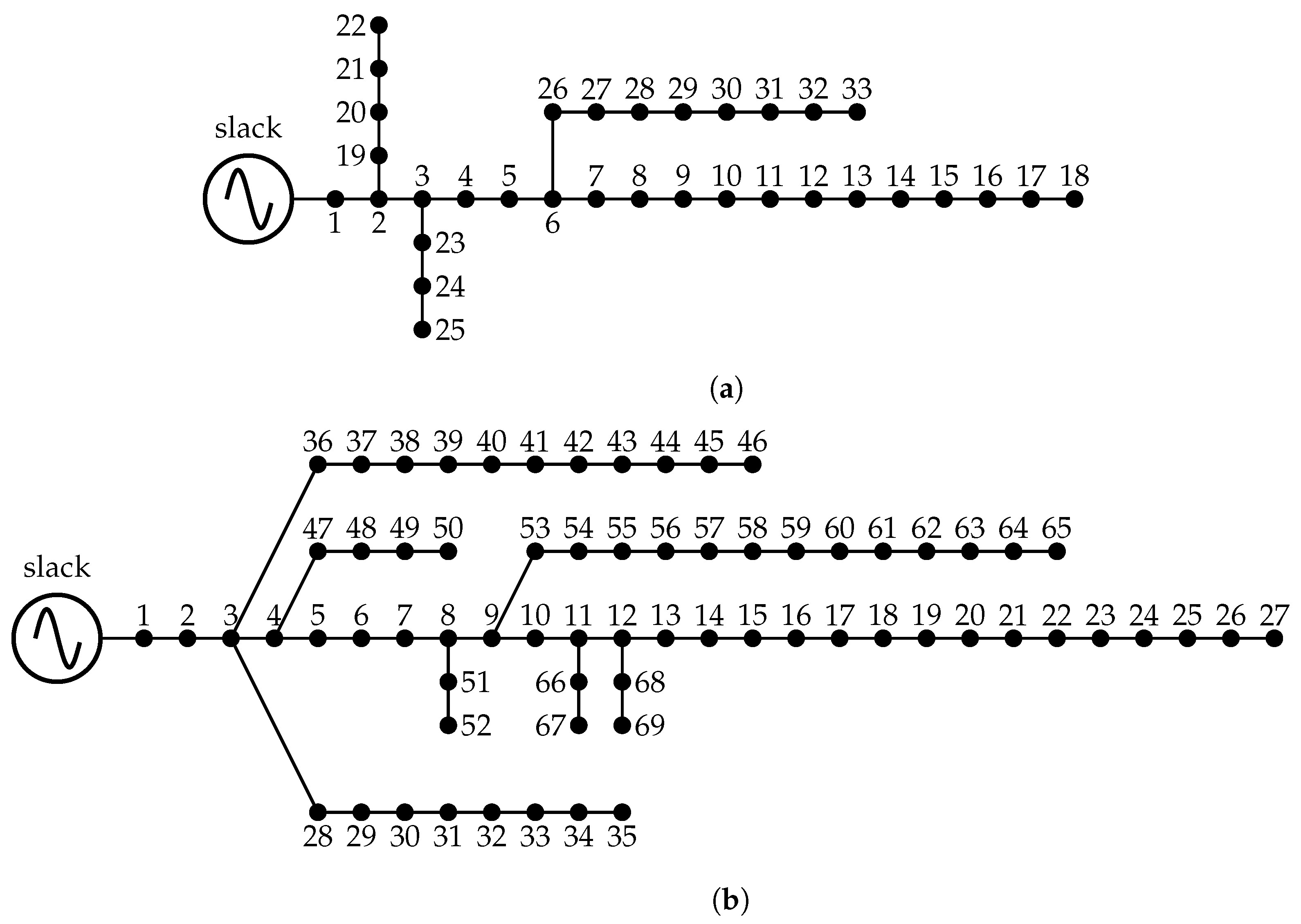
5. Test Systems and Comparative Methods

To verify that the SA method and the MBF load flow, two classical and well-known electrical distribution networks are employed composed of 33 and 69 buses configured with a radial connection. These test feeders are operated with a voltage magnitude of 12.66 kV at the slack source, which is positioned at bus 1 for both test feeders as depicted in Figure 1. Note that these systems were selected to evaluate the equivalence between the studied power flow approaches, as in the specialized literature, these systems are currently selected to implement different optimization strategies for distribution systems, such as the optimal location of distributed generators [16,20], optimal location of capacitor banks and static distribution compensators [21,22,23], and grid reconfiguration studies [24,25], among others.
The complete information regarding these test systems can be found in [16].
On the other hand, to verify that both methods are equivalent for load flow calculations in AC networks, we implement different load flow methods available in the scientific literature for distribution systems. These are the GS [6], the accelerate version of the Gauss–Seidel (AG) [7], the NR [26], and the Levenberg–Marquardt (LM) methods [27].

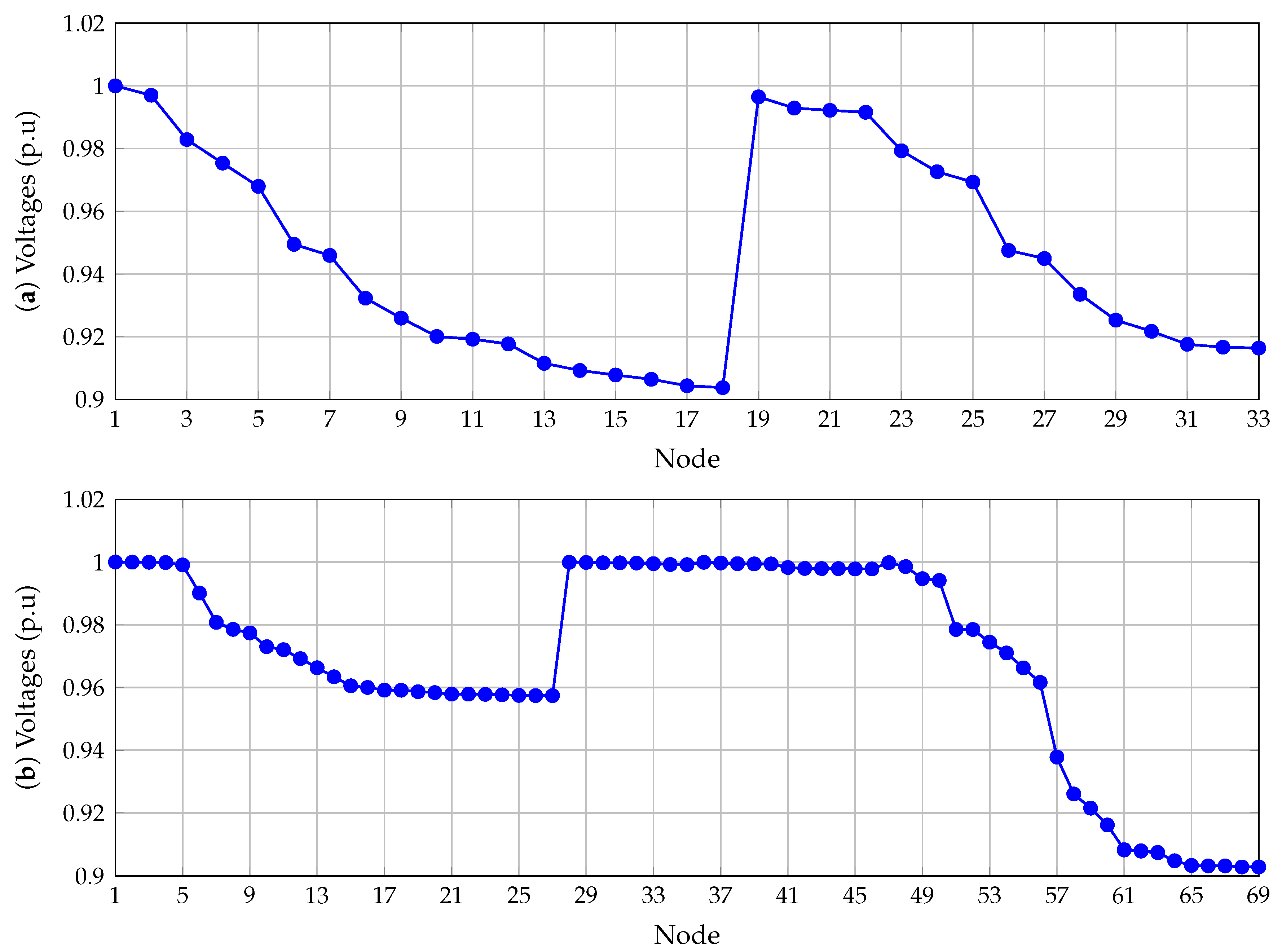
6. Numerical Validation

The numerical validations are implemented using a personal computer with an INTEL(R) Core(TM) i 7 7700 processor at 3.60 GHz, 8 GB RAM, running a 64-bits Windows 10 operative system. The simulation software used is MATLAB 2020b. In addition, the processing time presented in this research are the average values after 10,000 repetitions for the studied and comparative methods. Besides, to determine the effectiveness of each of the studied and comparative methods, we evaluate the amount of active power losses on the distribution network (see Equation (24)). Note that we consider ϵ = 1 × 10 10 as the convergence error between two consecutive iterations of voltage variables:
p loss = real J T Z p J = real V T Y V .
Table 1 reports the numerical results of the studied load flow methods, i.e., the SA and the MBF load flow approaches as well as the results of the comparative methods.
The results in Table 1 allows for the following remarks:
The conventional GS approach exhibits the worst performance in terms of processing times and the number of iterations required to solve the load flow problem in both test feeders. In addition, the accelerated version of the GS approach allows for improvement in its performance (i.e., the GS behavior) by reducing processing times by about 91.28 % and 94.66 % for the 33- and 69-bus distribution grids, while the number of iterations is reduced by about 90.19 % and 94.99 % respectively;
The classical NR and LM load flow approaches have the same numerical performance regarding the total iterations required to solve the load flow problem in both test feeders with 5 iterations in both cases. The low number of iterations in these methods is attributed to the fact that both work with the Jacobian matrix, which contains information about the direction of the maximum change of load flow equations, a situation that does not occur for the remainder of the load flow methods, as these do not use information of the derivatives of the load flow equations. With regard to processing times, the NR and LM methods are very similar, as in the case of the system with 33 buses, the difference is lower than 0.15 ms, and in the case of the system composed of 69 buses, this difference is about 4 41 ms;
The numerical results for the 33- and 69-node test feeders obtained for the SA and the MBF load flow methods, i.e., the equivalent load flow approaches, is the same regarding the number of iterations, as these take 10 iterations to solve the load flow problem in both test feeders however, regarding the processing times, we can observe that the SA is the faster approach as demonstrated in [12]. Even if both methods are equivalent, the SA approach calculates the admittance matrix, i.e., Y , using the direct method by adding the inverse of the conductance at this line, while the MBF method uses matricial calculations for the products between the incidence matrix and the primitive matrices, which consumes additional processing times.
It is also important to mention that regarding the estimation of the total grid losses, all the methods find an equal numerical solution with an error lower than 1 × 10 6 , which can be considered negligible for any practical purpose, which entails that all the approaches reported in Table 1 are suitable for solving the load flow problem in electrical distribution networks.
On the other hand, Table 2 presents the behavior of the convergence errors of the SA and the MBF load flow methods for the largest studied test feeder.
Note that the behavior of the convergence error in the 69-node test feeder listed in Table 2 confirms that the SA and MBF are completely equivalent load flow methods, as their recursive formulas have exactly the same numerical performance. Finally, Figure 2 presents the voltage profiles of both test feeders when the load flow is solved with the SA load flow method. These are completely equal for each one of the comparative methods listed in Table 1, as the convergence error of 1 × 10 10 is appropriate for each of them.

7. Conclusions

This paper made a comparative study of two recently developed load flow methodologies for AC electrical grids, which are the SA and MBF load flow methods. This comparative analysis, using admittance and incidence matrices, allowed us to demonstrate that both approaches were exactly the same, with the only difference being the way in which the recursive formulas (7) and (17) were obtained however, the matricial components on them were equal. Numerical simulations using two radial test feeders composed of 33 and 69 buses demonstrated that the number of iterations taken by the SA and MBF was the same, as the convergence error was exactly equal, which also confirmed that both load flow methodologies were completely equivalent. With regard to processing times, the SA approach had a small advantage, as the required number of calculations to obtain the admittance matrix was lower in comparison to the MBF, which clearly affected the final processing times of the second one.

Author Contributions

Conceptualization, methodology, software, and writing—review and editing, M.C.H.-B., O.D.M., H.R.C. and L.A.-B. All authors have read and agreed to the published version of the manuscript.

Funding

This work was supported in part by the Laboratorio de Simulación Hardware-in-the-loop para Sistemas Ciberfísicos under Grant TEC2016-80242-P (AEI/FEDER) and in part by the Spanish Ministry of Economy and Competitiveness under Grant DPI2016-75294-C2-2-R.

Institutional Review Board Statement

Not applicable.

Informed Consent Statement

Not applicable.

Data Availability Statement

No new data were created or analyzed in this study. Data sharing is not applicable to this article.

Acknowledgments

This work has been derived from the undergraduate project: “Formulación y comparación de cinco métodos para el análisis de flujo de potencia en sistemas de distribución AC en el software MATLAB®” presented by the student María Camila Herrera-Briñez to the Electrical Engineering Program of the Engineering Faculty at Universidad Distrital Francisco José de Caldas as a partial requirement for the Bachelor in Electrical Engineering.

Conflicts of Interest

The authors declare no conflict of interest.

References

  1. Abdi, H.; Beigvand, S.D.; Scala, M.L. A review of optimal power flow studies applied to smart grids and microgrids. Renew. Sustain. Energy Rev. 2017, 71, 742–766. [Google Scholar] [CrossRef]
  2. Lavaei, J.; Low, S.H. Zero Duality Gap in Optimal Power Flow Problem. IEEE Trans. Power Syst. 2012, 27, 92–107. [Google Scholar] [CrossRef] [Green Version]
  3. Marini, A.; Mortazavi, S.; Piegari, L.; Ghazizadeh, M.S. An efficient graph-based power flow algorithm for electrical distribution systems with a comprehensive modeling of distributed generations. Electr. Power Syst. Res. 2019, 170, 229–243. [Google Scholar] [CrossRef]
  4. Phongtrakul, T.; Kongjeen, Y.; Bhumkittipich, K. Analysis of Power Load Flow for Power Distribution System based on PyPSA Toolbox. In Proceedings of the 2018 15th International Conference on Electrical Engineering/Electronics, Computer, Telecommunications and Information Technology (ECTI-CON), Chiang Rai, Thailand, 18–21 July 2018. [Google Scholar] [CrossRef]
  5. Prabhu, J.A.X.; Sharma, S.; Nataraj, M.; Tripathi, D.P. Design of electrical system based on load flow analysis using ETAP for IEC projects. In Proceedings of the 2016 IEEE 6th International Conference on Power Systems (ICPS), New Delhi, India, 4–6 March 2016. [Google Scholar] [CrossRef]
  6. Grainger, J.J.; Stevenson, W.D. Power System Analysis; McGraw-Hill series in electrical and computer engineering: Power and energy; McGraw-Hill: New York, NY, USA, 2003. [Google Scholar]
  7. Gönen, T. Modern Power System Analysis; CRC Press: Boca Raton, FL, USA, 2016. [Google Scholar]
  8. Montoya, O.D.; Gil-González, W.; Giral, D.A. On the Matricial Formulation of Iterative Sweep Power Flow for Radial and Meshed Distribution Networks with Guarantee of Convergence. Appl. Sci. 2020, 10, 5802. [Google Scholar] [CrossRef]
  9. Shen, T.; Li, Y.; Xiang, J. A Graph-Based Power Flow Method for Balanced Distribution Systems. Energies 2018, 11, 511. [Google Scholar] [CrossRef] [Green Version]
  10. Garces, A. A Linear Three-Phase Load Flow for Power Distribution Systems. IEEE Trans. Power Syst. 2016, 31, 827–828. [Google Scholar] [CrossRef]
  11. Bocanegra, S.Y.; Gil-Gonzalez, W.; Montoya, O.D. A New Iterative Power Flow Method for AC Distribution Grids with Radial and Mesh Topologies. In Proceedings of the 2020 IEEE International Autumn Meeting on Power, Electronics and Computing (ROPEC), Ixtapa, Mexico, 4–6 November 2020. [Google Scholar] [CrossRef]
  12. Montoya, O.D.; Gil-González, W. On the numerical analysis based on successive approximations for power flow problems in AC distribution systems. Electr. Power Syst. Res. 2020, 187, 106454. [Google Scholar] [CrossRef]
  13. Li, Z.; Yu, J.; Wu, Q.H. Approximate Linear Power Flow Using Logarithmic Transform of Voltage Magnitudes With Reactive Power and Transmission Loss Consideration. IEEE Trans. Power Syst. 2018, 33, 4593–4603. [Google Scholar] [CrossRef]
  14. Montoya, O.D. On Linear Analysis of the Power Flow Equations for DC and AC Grids With CPLs. IEEE Trans. Circuits Syst. II Express Briefs 2019, 66, 2032–2036. [Google Scholar] [CrossRef]
  15. Molzahn, D.K.; Hiskens, I.A. Sparsity-Exploiting Moment-Based Relaxations of the Optimal Power Flow Problem. IEEE Trans. Power Syst. 2015, 30, 3168–3180. [Google Scholar] [CrossRef]
  16. Grisales-Noreña, L.; Montoya, D.G.; Ramos-Paja, C. Optimal Sizing and Location of Distributed Generators Based on PBIL and PSO Techniques. Energies 2018, 11, 1018. [Google Scholar] [CrossRef] [Green Version]
  17. Simpson-Porco, J.W.; Dorfler, F.; Bullo, F. On Resistive Networks of Constant-Power Devices. IEEE Trans. Circuits Syst. II Express Briefs 2015, 62, 811–815. [Google Scholar] [CrossRef] [Green Version]
  18. Montoya, O.D.; Garrido, V.M.; Gil-Gonzalez, W.; Grisales-Norena, L.F. Power Flow Analysis in DC Grids: Two Alternative Numerical Methods. IEEE Trans. Circuits Syst. II Express Briefs 2019, 66, 1865–1869. [Google Scholar] [CrossRef]
  19. Montoya, O.D. On the Existence of the Power Flow Solution in DC Grids With CPLs Through a Graph-Based Method. IEEE Trans. Circuits Syst. II Express Briefs 2020, 67, 1434–1438. [Google Scholar] [CrossRef]
  20. Kaur, S.; Kumbhar, G.; Sharma, J. A MINLP technique for optimal placement of multiple DG units in distribution systems. Int. J. Electr. Power Energy Syst. 2014, 63, 609–617. [Google Scholar] [CrossRef]
  21. Gil-González, W.; Montoya, O.D.; Rajagopalan, A.; Grisales-Noreña, L.F.; Hernández, J.C. Optimal Selection and Location of Fixed-Step Capacitor Banks in Distribution Networks Using a Discrete Version of the Vortex Search Algorithm. Energies 2020, 13, 4914. [Google Scholar] [CrossRef]
  22. Riaño, F.E.; Cruz, J.F.; Montoya, O.D.; Chamorro, H.R.; Alvarado-Barrios, L. Reduction of Losses and Operating Costs in Distribution Networks Using a Genetic Algorithm and Mathematical Optimization. Electronics 2021, 10, 419. [Google Scholar] [CrossRef]
  23. Montoya, O.D.; Gil-González, W.; Hernández, J.C. Efficient Operative Cost Reduction in Distribution Grids Considering the Optimal Placement and Sizing of D-STATCOMs Using a Discrete-Continuous VSA. Appl. Sci. 2021, 11, 2175. [Google Scholar] [CrossRef]
  24. Taher, S.A.; Karimi, M.H. Optimal reconfiguration and DG allocation in balanced and unbalanced distribution systems. Ain Shams Eng. J. 2014, 5, 735–749. [Google Scholar] [CrossRef] [Green Version]
  25. Priyadarshini, R.; Prakash, R.; Shankaralingappa, C.B. Network Reconfiguration of radial distribution network using Cuckoo Search Algorithm. In Proceedings of the 2015 Annual IEEE India Conference (INDICON), New Delhi, India, 17–20 December 2015. [Google Scholar] [CrossRef]
  26. Lagace, P.J.; Vuong, M.H.; Kamwa, I. Improving power flow convergence by Newton Raphson with a Levenberg-Marquardt method. In Proceedings of the 2008 IEEE Power and Energy Society General Meeting—Conversion and Delivery of Electrical Energy in the 21st Century, Pittsburgh, PA, USA, 20–24 July 2008; pp. 1–6. [Google Scholar]
  27. Milano, F. Analogy and Convergence of Levenberg’s and Lyapunov-Based Methods for Power Flow Analysis. IEEE Trans. Power Syst. 2016, 31, 1663–1664. [Google Scholar] [CrossRef]
Figure 1. Electrical configuration of the test feeders: (a) 33-node test system and (b) 69-node test system.
Applsci 11 02905 g001
Figure 2. Voltage profiles in the distribution networks under analysis: (a) 33-bus test system and (b) 69-bus test feeder.
Applsci 11 02905 g002
Table 1. Load flow results for both test feeders. Successive approximations (SA); Newton–Raphson (NR); Gauss–Seidel (GS); matricial backward/forward (MBF); and Levenberg–Marquardt (LM).
MethodProc. Time (ms)IterationsLosses (p.u)
Test system composed of 33 buses
GS441.97396023132.109785
AG ( α = 1.82 ) 38.5554032272.109785
NR10.75120352.109785
LM10.88165652.109785
MBF1.322962102.109785
SA0.518957102.109785
Test system composed of 69 buses
GS31107.756292490312.421523
AG ( α = 1.92 ) 1662.69079224552.421523
NR38.30308852.421523
LM42.71905552.421523
MBF5.369374102.421523
SA2.488095102.421523
Table 2. Behavior of the convergence errors.
IterationSAMBF
18.8223 × 10 2 8.8223 ×   10 2
28.0437 ×   10 3 8.0437 ×   10 3
37.5688 ×   10 4 7.5688 ×   10 4
47.5134 ×   10 5 7.5134 ×   10 5
57.1145 ×   10 6 7.1145 ×   10 6
67.0636 ×   10 7 7.0636 ×   10 7
76.6881 ×   10 8 6.6881 ×   10 8
86.6400 ×   10 9 6.6400 ×   10 9
96.2870 ×   10 10 6.2870 ×   10 10
106.2418 ×   10 11 6.2418 ×   10 11
Publisher’s Note: MDPI stays neutral with regard to jurisdictional claims in published maps and institutional affiliations.

