
Trichomonas vaginalis Detection Using Two Convolutional Neural Networks with Encoder-Decoder Architecture


Abstract
1. Introduction
2. Related Works
3. Method
3.1. Convolutional Neural Network Based on Encoder-Decoder Architecture for Rough Detection
3.1.1. Encoder
3.1.2. Decoder
3.1.3. Training
3.1.4. Inference
3.2. Convolutional Neural Network Based on Encoder-Decoder Architecture for Fine Detection
3.2.1. Encoder and Decoder
3.2.2. Training
3.2.3. Inference
4. Experimental Results
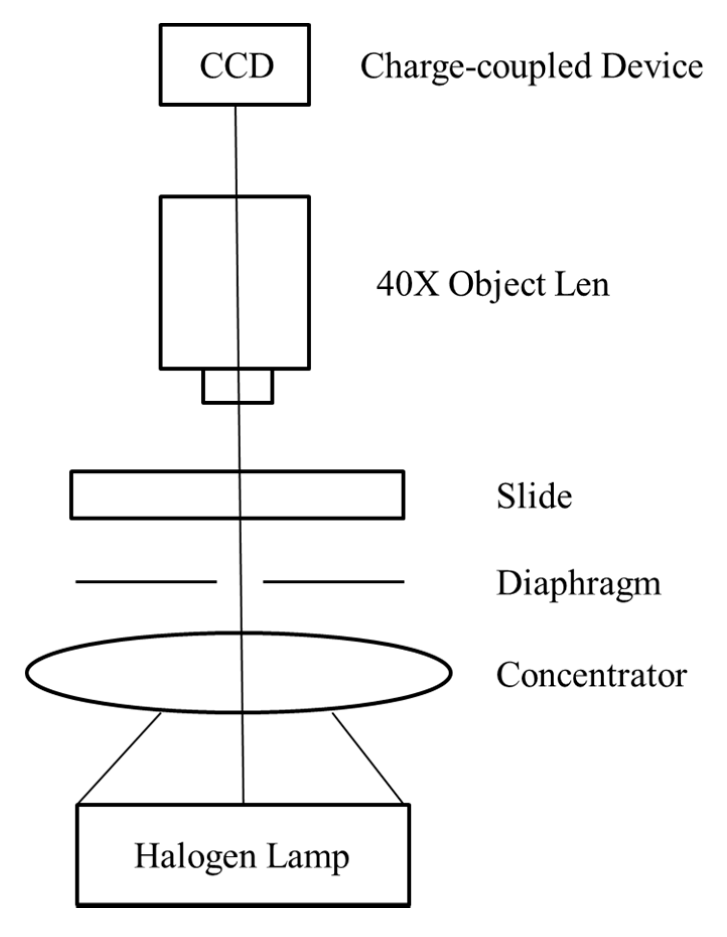
4.1. Dataset and Optical System
4.2. Metric
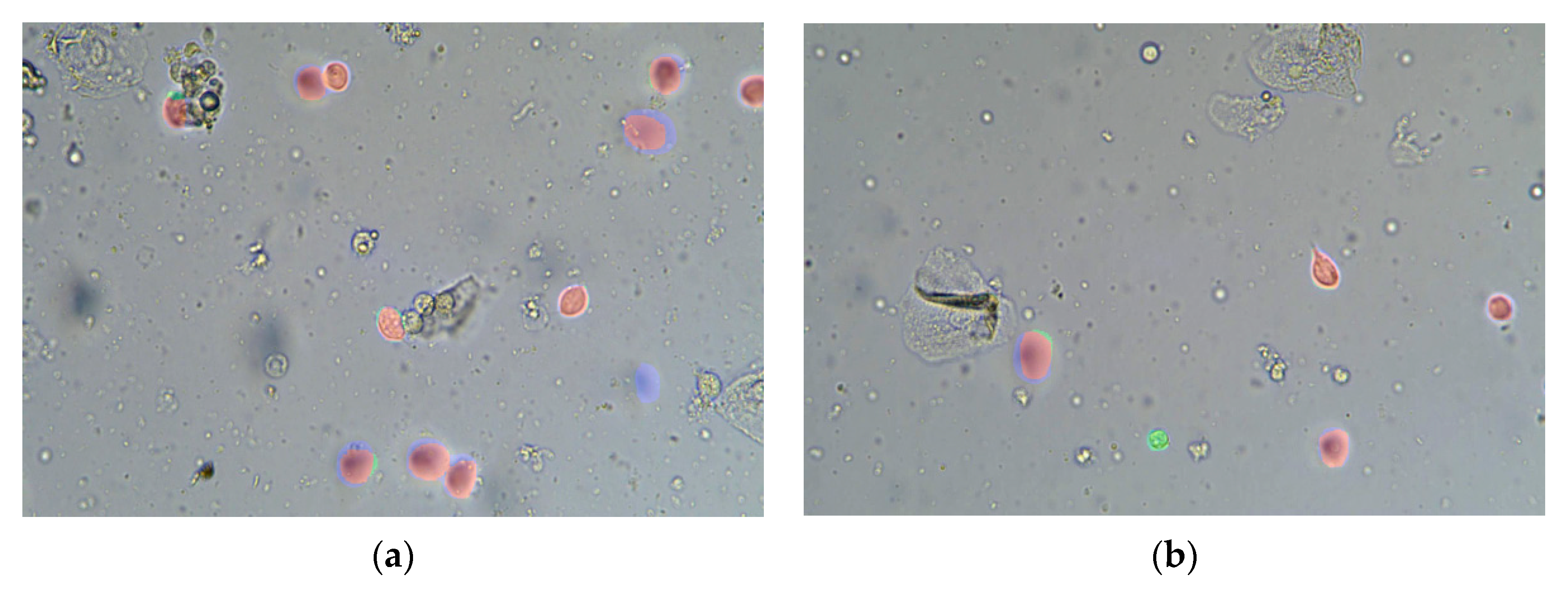
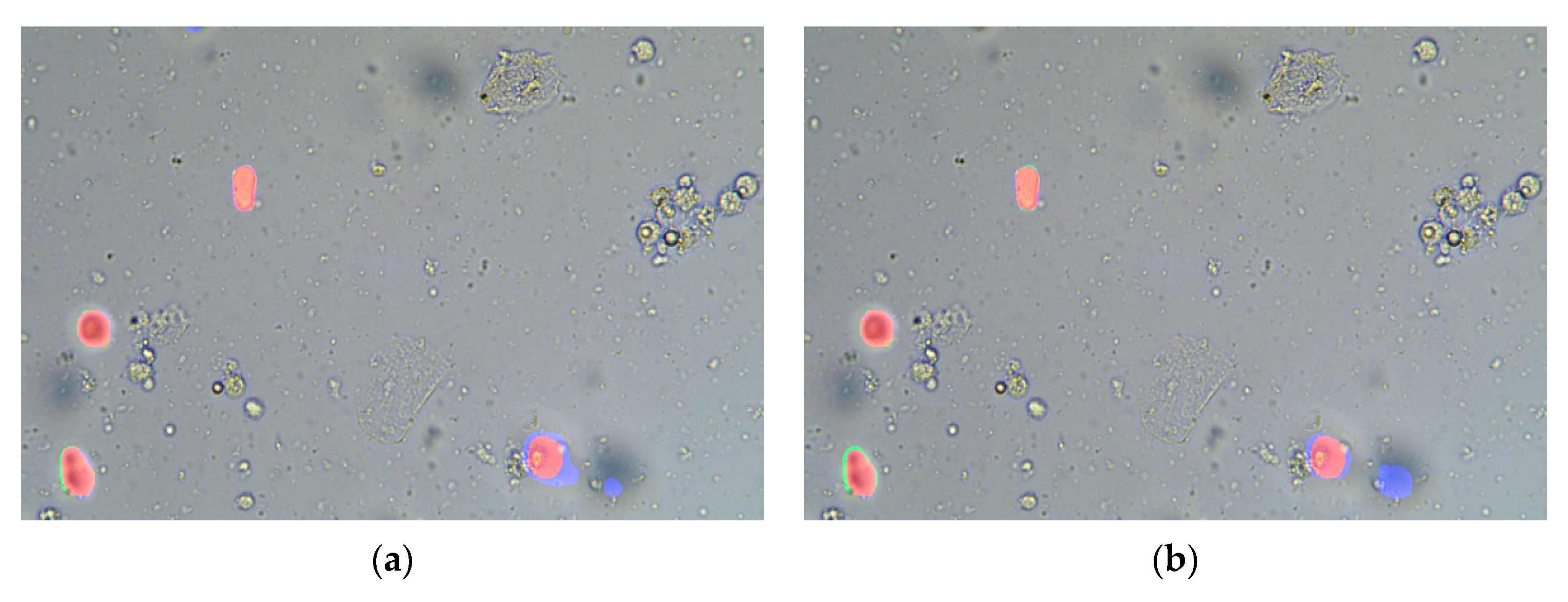
4.3. Results
4.4. The Operating Environment and Running Times
5. Discussion
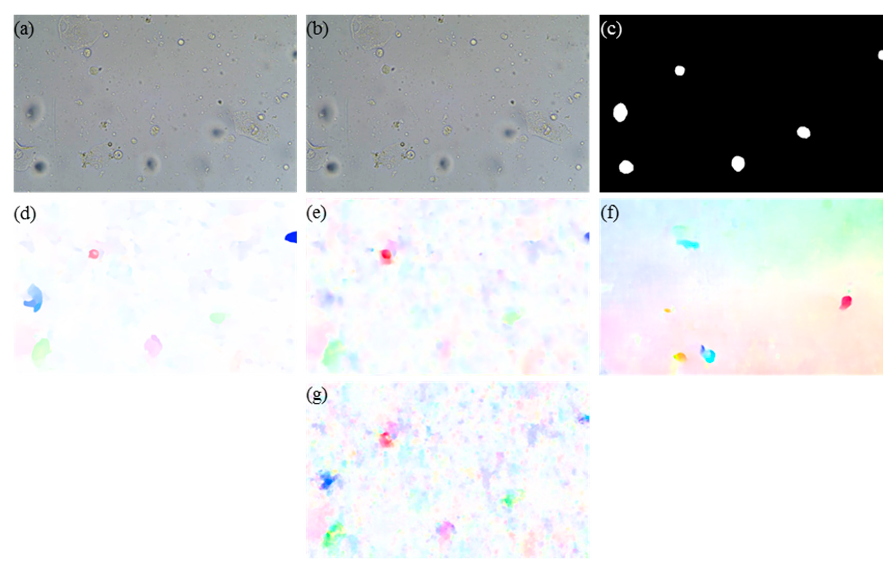
5.1. Selection of the Optical Flow Calculation Method
5.2. Ablation Study
5.2.1. Network Architecture
5.2.2. Attention Module
5.2.3. Network Inputs
5.3. Comparison with Traditional Video Object Detection Methods
5.4. The Performance of the Rough Detection Network Using Different Outputs
5.5. Limitations of Our Trichomonas Vaginalis Detection Method
6. Conclusions
Supplementary Materials
Author Contributions
Funding
Institutional Review Board Statement
Informed Consent Statement
Data Availability Statement
Acknowledgments
Conflicts of Interest
References
- Hao, R.; Wang, X.; Zhang, J.; Liu, J.; Ni, G.; Du, X.; Liu, L.; Liu, Y. Automatic detection of trichomonads based on an improved Kal-man background reconstruction algorithm. JOSA A 2017, 34, 752–759. [Google Scholar] [CrossRef] [PubMed]
- Du, X.; Liu, L.; Wang, X.; Zhang, J.; Ni, G.; Hao, R.; Liu, J.; Liu, Y. Trichomonas Detection in Leucorrhea Based on VIBE Method. Comput. Math. Methods Med. 2019, 2019, 1–10. [Google Scholar] [CrossRef] [PubMed]
- Jain, R.; Nagel, H.-H. On the Analysis of Accumulative Difference Pictures from Image Sequences of Real World Scenes. IEEE Trans. Pattern Anal. Mach. Intell. 1979, 1, 206–214. [Google Scholar] [CrossRef] [PubMed]
- Yang, M.-M.; Guo, Q.-P. A motion detection algorithm based on three frame difference and background difference. In Proceedings of the 8th International Symposium on Distributed Computing and Applications to Business Engineering and Science, Wuhan, China, 16–19 October 2009; pp. 487–490. [Google Scholar]
- Stauffer, C.; Grimson, W. Adaptive background mixture models for real-time tracking. In Proceedings of the 1999 IEEE Computer Society Conference on Computer Vision and Pattern Recognition (Cat. No PR00149), Fort Collins, CO, USA, 23–25 June 2003; Institute of Electrical and Electronics Engineers (IEEE): New York, NY, USA; Volume 2, p. 257. [Google Scholar]
- Barnich, O.; Vanogenbroeck, M. ViBe: A powerful random technique to estimate the background in video sequences. In Proceedings of the IEEE International Conference on Acoustics, Speech & Signal Processing, Taipei, Taiwan, 19–24 April 2009; pp. 945–948. [Google Scholar]
- Xu, L.; Jia, J.; Matsushita, Y. Motion Detail Preserving Optical Flow Estimation. IEEE Trans. Pattern Anal. Mach. Intell. 2012, 34, 1744–1757. [Google Scholar] [CrossRef] [PubMed]
- Zhu, X.; Xiong, Y.; Dai, J.; Yuan, L.; Wei, Y. Deep Feature Flow for Video Recognition. In Proceedings of the 2017 IEEE Conference on Computer Vision and Pattern Recognition (CVPR), Honolulu, HI, USA, 21–26 July 2017; pp. 4141–4150. [Google Scholar]
- Zhu, X.; Wang, Y.; Dai, J.; Yuan, L.; Wei, Y. Flow-Guided Feature Aggregation for Video Object Detection. In Proceedings of the 2017 IEEE International Conference on Computer Vision (ICCV), Venice, Italy, 22–29 October 2017; pp. 408–417. [Google Scholar]
- Zhu, X.; Dai, J.; Yuan, L.; Wei, Y. Towards High Performance Video Object Detection. In Proceedings of the 2018 IEEE/Cvf Conference on Computer Vision and Pattern Recognition, Salt Lake City, UT, USA, 18–23 June 2018; pp. 7210–7218. [Google Scholar]
- Dosovitskiy, A.; Fischer, P.; Ilg, E.; Hausser, P.; Hazirbas, C.; Golkov, V.; Van Der Smagt, P.; Cremers, D.; Brox, T. FlowNet: Learning Optical Flow with Convolutional Networks. In Proceedings of the 2015 IEEE International Conference on Computer Vision, Santiago, Chile, 7–13 December 2015; pp. 2758–2766. [Google Scholar]
- Simonyan, K.; Zisserman, A. Very deep convolutional networks for large-scale image recognition. arXiv 2014, arXiv:1409.1556. [Google Scholar]
- Hui, T.W.; Tang, X.; Loy, C.C. A lightweight optical flow CNN-revisiting data fidelity and regularization. arXiv 2019, arXiv:1903.07414. [Google Scholar] [CrossRef] [PubMed]
- Hu, J.; Shen, L.; Sun, G. Squeeze-and-excitation networks. In Proceedings of the IEEE Conference on Computer Vision and Pattern Recognition, Las Vegas, NV, USA, 27–30 June 2018; pp. 7132–7141. [Google Scholar]
- Kingma, D.P.; Ba, J. Adam: A method for stochastic optimization. In Proceedings of the International Conference Learn, San Diego, CA, USA, 5–8 May 2015. [Google Scholar]
- Lin, T.Y.; Goyal, P.; Girshick, R.; He, K.; Dollar, P. Focal loss for dense object detection. In Proceedings of the IEEE international conference on computer vision (ICCV), Venice, Italy, 22–29 October 2017; pp. 2980–2988. [Google Scholar]
- Perazzi, F.; Khoreva, A.; Benenson, R.; Schiele, B.; Sorkine-Hornung, A. Learning Video Object Segmentation from Static Images. In Proceedings of the 2017 IEEE Conference on Computer Vision and Pattern Recognition (CVPR) IEEE, Honolulu, HI, USA, 21–26 July 2017; pp. 3491–3500. [Google Scholar]
- Bookstein, F.; Green, W.D.K. A Thin-plate splines and the decomposition of deformations. Math. Methods Med. Imaging 1993, 2, 14–28. [Google Scholar]
- Ilg, E.; Mayer, N.; Saikia, T.; Keuper, M.; Dosovitskiy, A.; Brox, T. FlowNet 2.0: Evolution of Optical Flow Estimation with Deep Networks. In Proceedings of the 2017 IEEE Conference on Computer Vision and Pattern Recognition (CVPR), Honolulu, HI, USA, 21–26 July 2017; Institute of Electrical and Electronics Engineers (IEEE): New York, NY, USA; pp. 1647–1655. [Google Scholar]
- Sun, D.; Yang, X.; Liu, M.-Y.; Kautz, J. PWC-Net: CNNs for Optical Flow Using Pyramid, Warping, and Cost Volume. In Proceedings of the 2018 IEEE/CVF Conference on Computer Vision and Pattern Recognition, Salt Lake City, UT, USA, 18–23 June 2018; pp. 8934–8943. [Google Scholar]
- Ranjan, A.; Black, M.J. Optical flow estimation using a spatial pyramid network. In Proceedings of the IEEE Conference on Computer Vision and Pattern Recognition (CVPR), Honolulu, HI, USA, 21–26 July 2017; pp. 4161–4170. [Google Scholar]
- He, K.; Zhang, X.; Ren, S.; Sun, J. Deep residual learning for image recognition. arXiv 2015, arXiv:1512.03385. [Google Scholar]
- Chen, L.C.; Zhu, Y.; Papandreou, G.; Schroff, F.; Adam, H. Encoder-decoder with atrous separable convolution for semantic im-age segmentation. In Proceedings of the European Conference on Computer Vision (ECCV), Munich, Germany, 8–14 September 2018; pp. 801–818. [Google Scholar]
- Wang, X.; Girshick, R.; Gupta, A.; He, K. Non-local Neural Networks. In Proceedings of the 2018 IEEE/CVF Conference on Computer Vision and Pattern Recognition, Salt Lake City, UT, USA, 18–23 June 2018; Institute of Electrical and Electronics Engineers (IEEE): New York, NY, USA; pp. 7794–7803. [Google Scholar]
- Woo, S.; Park, J.; Lee, J.Y.; Kweon, I.S. Cbam: Convolutional block attention module. In Proceedings of the European conference on computer vision (ECCV), Munich, Germany, 8–14 September 2018; pp. 3–19. [Google Scholar]
- Fu, J.; Liu, J.; Tian, H.; Li, Y.; Bao, Y.; Fang, Z.; Lu, H. Dual Attention Network for Scene Segmentation. In Proceedings of the 2019 IEEE/CVF Conference on Computer Vision and Pattern Recognition (CVPR), Long Beach, CA, USA, 16–20 June 2019; Institute of Electrical and Electronics Engineers (IEEE): New York, NY, USA; pp. 3141–3149. [Google Scholar]


| Video Name | Video1 | Video2 | Video3 | Video4 | Video5 | Video6 |
|---|---|---|---|---|---|---|
| Frame number | 221 | 250 | 406 | 498 | 433 | 712 |
| Video Name | Mean Recall | Mean Precision | Mean IoU | |
|---|---|---|---|---|
| Training set | video1 | 92.76% | 85.81% | 80.04% |
| video2 | 90.71% | 84.96% | 77.91% | |
| Validation set | video3 | 84.62% | 83.66% | 72.08% |
| Test set | video4 | 89.84% | 74.28% | 67.94% |
| video5 | 92.73% | 75.79% | 71.32% | |
| video6 | 89.44% | 78.26% | 71.51% |
| Video Name | Mean Recall | Mean Precision | Mean IoU | Mean Average IoU | |
|---|---|---|---|---|---|
| Training set | video1 | 89.35% | 89.35% | 80.19% | 78.14% |
| video2 | 90.38% | 84.14% | 76.09% | ||
| Validation set | video3 | 84.20% | 85.33% | 73.12% | 73.12% |
| Test set | video4 | 89.65% | 78.86% | 70.13% | 72.09% |
| video5 | 92.06% | 78.59% | 73.34% | ||
| video6 | 86.45% | 82.30% | 72.80% |
| Optical Flow Calculation | Slicing | Rough Detection | Fine Detection | Total | |
|---|---|---|---|---|---|
| Running times | 0.545 s | 0.050 s | 1.556 s | 0.875 s | 3.026 s |
| Architecture Variant | The Optimal Value of Mean IoU on Validation Set (Video3) | |
|---|---|---|
| FlowNetSimple [11] | None | 68.19% |
| Encoder changed | VGG16 [12] | 71.50% |
| Resnet50 [22] | 68.31% | |
| modified Xception [23] | 64.99% | |
| Attention blocks added | VGG16 [12] + SE [14] | 72.08% |
| Attention Module Added | Video3 | Video4 | Video5 | Video6 |
|---|---|---|---|---|
| None | 71.50% | 67.75% | 70.60% | 69.76% |
| +SE [14] | 72.08% | 67.94% | 71.32% | 71.51% |
| +Non Local [24] | 71.73% | 66.64% | 69.65% | 67.81% |
| +CBAM [25] | 70.75% | 66.82% | 70.62% | 71.25% |
| +DA [26] | 71.16% | 66.90% | 70.80% | 70.37% |
| Input Information | Video3 | Video4 | Video5 | Video6 |
|---|---|---|---|---|
| Two adjacent frames (6 channels) | 71.52% | 66.51% | 67.49% | 68.18% |
| Two adjacent frames with optical flow (8 channels) | 70.94% | 67.87% | 69.51% | 67.92% |
| Three consecutive frames with optical flow (13 channels) | 71.50% | 67.75% | 70.60% | 69.76% |
| Five consecutive frames with optical flow (23 channels) | 71.86% | 66.86% | 67.86% | 67.12% |
| Method | Video1 | Video2 | Video3 | Video4 | Video5 | Video6 |
|---|---|---|---|---|---|---|
| Three frame difference [4] | 34.60% | 28.07% | 27.39% | 32.33% | 33.34% | 39.23% |
| GMM model [5] | 45.51% | 35.26% | 34.87% | 39.97% | 44.99% | 36.76% |
| Improved Kalman [1] | 44.52% | 39.87% | 39.48% | 42.95% | 47.93% | 51.15% |
| Improved VIBE [2] | 55.51% | 51.74% | 53.29% | 56.82% | 58.71% | 57.73% |
| This paper | 80.19% | 76.09% | 73.12% | 70.13% | 73.34% | 72.80% |
| Output | Video1 | Video2 | Video3 | Video4 | Video5 | Video6 |
|---|---|---|---|---|---|---|
| output1 | 80.04% | 77.91% | 72.08% | 67.94% | 71.32% | 71.51% |
| output2 | 80.02% | 77.95% | 72.00% | 67.85% | 71.28% | 71.25% |
| output3 | 79.41% | 77.40% | 71.64% | 67.53% | 71.05% | 70.83% |
| output4 | 76.19% | 74.77% | 70.76% | 65.78% | 68.84% | 68.15% |
| output5 | 75.96% | 73.40% | 70.42% | 65.30% | 68.40% | 68.09% |
Publisher’s Note: MDPI stays neutral with regard to jurisdictional claims in published maps and institutional affiliations. |
© 2021 by the authors. Licensee MDPI, Basel, Switzerland. This article is an open access article distributed under the terms and conditions of the Creative Commons Attribution (CC BY) license (http://creativecommons.org/licenses/by/4.0/).
Share and Cite
Wang, X.; Du, X.; Liu, L.; Ni, G.; Zhang, J.; Liu, J.; Liu, Y. Trichomonas vaginalis Detection Using Two Convolutional Neural Networks with Encoder-Decoder Architecture. Appl. Sci. 2021, 11, 2738. https://doi.org/10.3390/app11062738
Wang X, Du X, Liu L, Ni G, Zhang J, Liu J, Liu Y. Trichomonas vaginalis Detection Using Two Convolutional Neural Networks with Encoder-Decoder Architecture. Applied Sciences. 2021; 11(6):2738. https://doi.org/10.3390/app11062738
Chicago/Turabian StyleWang, Xiangzhou, Xiaohui Du, Lin Liu, Guangming Ni, Jing Zhang, Juanxiu Liu, and Yong Liu. 2021. "Trichomonas vaginalis Detection Using Two Convolutional Neural Networks with Encoder-Decoder Architecture" Applied Sciences 11, no. 6: 2738. https://doi.org/10.3390/app11062738
APA StyleWang, X., Du, X., Liu, L., Ni, G., Zhang, J., Liu, J., & Liu, Y. (2021). Trichomonas vaginalis Detection Using Two Convolutional Neural Networks with Encoder-Decoder Architecture. Applied Sciences, 11(6), 2738. https://doi.org/10.3390/app11062738