Abstract
To overcome the difficulty of extracting the feature frequency of early bearing faults, this paper proposes an adaptive feature extraction scheme. First, the improved intrinsic time-scale decomposition, proposed in this paper, is used as a noise reduction method. Then, we use the adaptive composite quantum morphology analysis method, also proposed in this paper, to perform an adaptive demodulation analysis on the signal, and finally, extract the fault characteristics in the envelope spectrum. The experimental results show that the scheme performs well in the early fault feature extraction of rolling bearings.
1. Introduction
Rolling bearings are widely used mechanical parts which are often seen in high-speed, high-load, and other complex conditions [1]. They are also one of the most fault-prone parts. The operation of rolling bearings is easily disturbed by the environment. The collected signal characteristic components can easily be drowned out by strong background noise, especially in the early stage of failure. The fault diagnosis method based on vibration signal analysis is one of the most widely used and effective means to detect rolling bearing faults [2]. Employing an effective signal processing algorithm to extract the fault characteristics of the signal from the original signal with strong interference is key in the effective fault diagnosis of rolling bearings. In modern signal processing techniques, the most commonly used rotating machinery fault diagnosis techniques include empirical mode decomposition [3], wavelet transform [4], singular value decomposition [5], stochastic resonance [6], Principal Component Analysis (PCA) [7], Relative Principal Component Analysis [8], and advanced machine learning models [9,10]. However, they are limited in some respects; for instance, they lack adaptive signal processing. An adaptive time-frequency analysis method called intrinsic time decomposition (ITD) was proposed by Feri et al. [11], and is now widely utilized in the fault diagnosis of rotating machinery. ITD does not require envelope fitting iterations compared to EMD and its extension algorithm, and only linear interpolation is performed, so the operation is faster, and the modal mixing is improved compared to EMD and its extension algorithm [12].
In recent years, researchers have made many improvements to the ITD algorithm. A diesel engine fault identification method based on fully integrated intrinsic time-scale decomposition was proposed by Zhang et al. [13]. Xing et al. investigated the decomposition of gearbox vibration signal using the ITD method [14]. Hu et al. proposed a new approach, the time-scale decomposition of set cost sign, improving the envelope fitting method of ITD, which could prevent signal distortion [15]. Liu et al. utilized intrinsic time-scale decomposition to analyze diesel engine signals [16]. Bi et al. proposed the complete ensemble improved intrinsic time-scale decomposition (CEIITD) and bi-spectrum algorithms [17]. A new approach called the sparse coding shrinkage method was proposed by Yu et al. [18]. This method uses intrinsic time-scale decomposition as a sparse representation to extract pulse components from bearing vibration signals. An improved intrinsic time-scale decomposition (IITD) was proposed by Liu et al. [19]. Li et al. proposed a new method to extract ship-radiated noise features using the ITD method [20]. Yuan et al. proposed a method based on wavelet transform and added it to the iterative process of intrinsic time-scale decomposition to improve the signal-to-noise ratio of the decomposed signal [21].
At present, the envelope method of ITD is fixed throughout the decomposition process. However, the waveform and fluctuation trend of the maximum and minimum mode components obtained by each decomposition may be completely different from that of the original signal. It is, therefore, best to allow the utilization of different envelope interpolation algorithms during the generation of each rotating component. An envelope fitting method that could obtain better decomposition results for all signals is still needed. Given these factors, a novel decomposition method called improved intrinsic time-scale decomposition (IITD) was designed and applied to the complete ensemble intrinsic time-scale with adaptive noise (CEITDAN) framework. This method combines the advantages of several common envelope fitting methods, and is different from the established method using a fixed envelope interpolation algorithm. In the screening process, the appropriate envelope interpolation algorithm could be automatically selected from multiple envelope interpolation algorithms by utilizing bandwidth criteria. Compared with the traditional method, the obtained decomposition results could effectively avoid the problem of curve distortion and the endpoint effect. This makes up for the lack of present ITD research and will reference subsequent related research. The proposed method in this paper differs from the literature [22] in its iterative approach in the decomposition process in that the literature [22] excludes irrelevant mode components by correlation coefficients of the mode components with the original signal, while the proposed method in this paper only targets the calculation of the bandwidth of the mode components themselves to determine whether they are irrelevant or not. The correlation coefficient is susceptible to interference under strong background noise compared to the bandwidth, so the bandwidth parameter used in the proposed method is more appropriate than the correlation coefficient. We named it ‘improved complete ensemble intrinsic time-scale with adaptive noise’ (ICEITDAN).
ICEITDAN could be regarded as a new denoising method in this program. It can eliminate the frequency component independent of the fault and highlight the frequency of the fault. In addition, we also need a method to demodulate and analyze the reconstructed signal to reduce the effect of residual noise on fault frequency extraction. In recent years, a number of scholars have introduced mathematical morphology from the field of image processing to the analysis of mechanical vibration signals, providing a new way to process nonlinear and unstable signals [23,24,25]. In mathematical morphological calculation, the selection of parameters and types of structural elements is important. If the optimal size parameters of the structural unit cannot be obtained while only employing empirical parameters, the performance of the algorithm will be greatly reduced.
To solve the problem of adaptive control with uncertain structure size, inspired by Reference [26] we proposed a demodulation method named composite quantum morphology analysis (CQMA). The signal is demodulated to extract the fault frequency. According to Reference [26], quantum signal processing frameworks could exploit the principles of quantum mechanics, various axioms, and constraints to develop new or modify established signal processing algorithms. Therefore, quantum entanglement theory could optimize the size of structural elements adaptively in morphological analysis. In the case of multiple signals, the local feature conversion of structural element size could be realized. In addition, quantum signal processing theory could improve the calculation efficiency of the adaptive structural unit size. The CQMA proposed in this paper includes two steps: Firstly, the amplitude and frequency modulation components of the reconstructed signal are analyzed by the demodulation method. Secondly, the fault characteristic frequency is obtained by envelope spectrum transformation. Compared with the traditional demodulation wavelet transform [27] and Teager–Kaiser energy operator [28], the proposed method achieves a higher demodulation performance. The results show that the reconstructed signal obtained by CQMA demodulation with the ICEITDAN method has strong practicability.
The remainder of this article is organized as follows: The second part introduces the method that is proposed in this article and the original method. The third part evaluates the performance of the ICEITDAN and CQMA (ICEITDAN-CQMA) methods through numerical simulation and experimental signals. Finally, the conclusions of this study are presented in the fourth part.
2. Proposed Fault Feature Extraction Methodology for the Fault Diagnosis of Rolling Bearings
Inspired by the advantages of ICEITDAN and CQMA, an ICEITDAN-CQMA technology for bearing fault detection is proposed. The steps are as follows:
- (1)
- Apply ICEITDAN to fault signals and obtain a series of goal proper rotation components (GPRCs).
- (2)
- Calculate the periodic modulation components to the generalized interference (PMGI) value of each GPRC.
- (3)
- Select the first three components with the highest PMGI value among the GPRCs and reconstruct them for further analysis.
- (4)
- Determine the scale range of CQMA and perform the CQMA operation for the main components that were obtained in step 3.
- (5)
- Use the envelope spectrum of the result of the CQMA analysis to extract the fault feature frequency.
The scheme that is proposed in this paper includes two steps: ICEITDAN noise reduction and demodulation analysis that is based on the composite quantum morphology analysis. The process of the ICEITDAN method will be introduced in detail in Section 2.2. For more detailed information on composite quantum morphological analysis-related theories and fault feature extraction methods for rolling bearing fault diagnosis, please refer to Section 2.3 and Section 2.4.
2.1. Preview of the ITD Method
ITD can accurately extract the instantaneous features of the signal in real-time and decompose the nonstationary signal to be analyzed into a series of proper rotation components (PRCs) and a residual trend component. The steps are as follows [11]:
Define as a set of original signals; L is defined as a baseline extraction operator. The mean value curve of the signal is expressed as or can be abbreviated as ; then, and can be obtained from the signal via ITD decomposition, and is defined as a reasonable PR component.
- (1)
- Determine the extreme value and the corresponding time of the original signal, , wherein is the number of extreme points; the piecewise linear baseline extraction operator of the signal is defined as follows:where and is the gain control parameter for extracting the amplitude of the intrinsic rotation component for control, which satisfies and is typically set to 0.5 [7].
- (2)
- By subtracting the baseline component from the original signal, the inherent rotation component can be calculated as follows:
- (3)
- Regarding as the original signal of the next step, repeat the above steps to decompose until the baseline component is monotonous.
- (4)
- After several ITD operations, the original signal is decomposed into several PR components and the sum of a monotone trend; the decomposition result is expressed as follows:where is the PR component of layer , is the baseline component of layer , and is the proper rotation component that is obtained via decomposition. is the residual signal.
2.2. Signal Denoising Using the Proposed IITD and ICEITDAN
To solve the problems of end effects and envelope fitting distortion, the ITD algorithm is improved. After identifying all the poles, each set of three adjacent poles is averaged to solve the problem of curve distortion, due to a single pole, and B-spline curve interpolation [29], linear interpolation [30], and cubic Hermite interpolation are applied. Although the interpolation algorithm [31] is used, to solve the fitting problem that is caused by the single use of the three methods, this paper utilizes the orthogonal combination method to construct a new interpolation algorithm to fit the envelope of the signal decomposition, and both can be retained. The advantages of interpolation methods can be complementary. The steps of the method are as follows:
Step 1: First, all the extremal points of the original signal shall be determined and denoted as , .
Step 2: Calculate the weighted average for each set of adjacent three extreme points and define and as follows:
To suppress the end effect, the mirror symmetry continuation method is used to extend the sequence endpoint, and the extreme values of the left and right ends are thereby obtained. is valued as 0 and k − 1, and endpoints and are obtained via Equations (5) and (6), respectively;
Step 3: Calculate all and by calculating the b-spline interpolation , linear interpolation , and cubic Hermite interpolation , then calculate , ,.
Step 4: Separate the three that were obtained from the signal to obtain three initial proper rotation components (IPRCs), then select an IPRC as the first component if it satisfies the proper rotation component (PRC) criterion; otherwise, the above steps must be repeated with the residue component as the original signal until each result can be an IPRC.
Step 5: Select the mode component with the minimum frequency bandwidth according to the literature [30] to obtain the result with minimum noise interference. Therefore, the minimum frequency bandwidth is used as the criterion for judging the rotational component of the target object. Select the target PRC from the IPRCs to be defined as GPRC1.
Step 6: Subtract GPRC1 from signal to obtain the residual error and use as a new pending signal. Repeat the above five steps until becomes a monotonic function or constant. The criterion for the judgment of the PRC adopts three thresholding methods [26].
In ITD, envelope selection is directly related to the decomposition accuracy of the rotational component, and a more accurate PRC can be generated through the use of a better envelope interpolation algorithm. We use reliable criteria in the screening process to select a suitable envelope interpolation algorithm. According to the literature [32], we need a standard for evaluating the performances of various envelope interpolation algorithms and identifying the best algorithm. Therefore, we use the bandwidth of the center instantaneous frequency, as proposed in Reference [33], as a reference to evaluate PRCS. The envelope interpolation algorithm that is used can be evaluated to determine the minimum bandwidth value relative to the center. The screening process is repeated, and unsuitable envelope interpolation algorithms are excluded from each decomposition. Therefore, the envelope error can be reduced, and a more accurate decomposition result can be obtained. Via this approach, we can select the best envelope fitting algorithm from the selected envelope interpolation algorithms. More accurate decomposition results can be obtained. Facilitated by the definition of GPRC, we can select a suitable envelope interpolation algorithm for minimizing each screening process, avoiding ITD curve distortion and end effect problems, and further weakening the mode mixing of the decomposition results. The flowchart is shown in Figure 1. The ideological framework of the CEITDAN method originates from the method that was proposed by the author in 2020 [34].
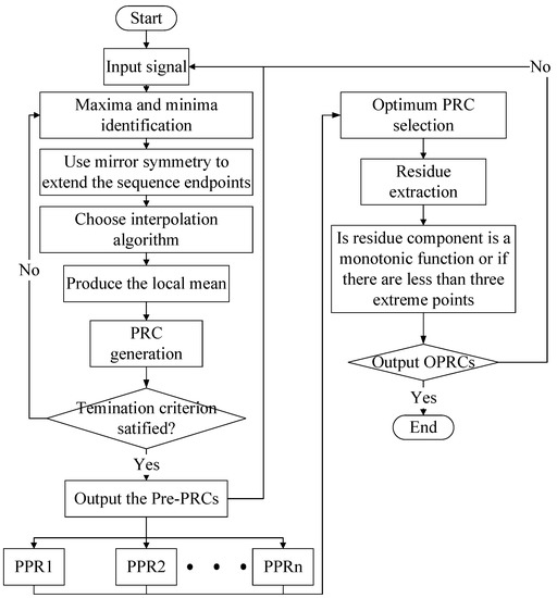
Figure 1.
Flowcharts diagram of the improved intrinsic time-scale decomposition (IITD) method.
2.3. Preview of the Mathematical Morphology Analysis and Quantum Signal Processing
2.3.1. Mathematical Morphology Analysis
Mathematical morphology methods realize satisfactory signal processing performance. Studies have shown that [35,36,37] the lengths of structural elements strongly impact their analysis. Vibration signals are usually composed of one or more groups of discrete signals. The common basic mathematical morphological operators are the expansion, erosion, opening, and closing operators, along with combinatorial variant operators among them. Assuming that is a one-dimensional discrete signal, it is defined as and ;
is a structural element; its definition domain is set as , where and . Then, the erosion operation and dilation operation of signal with respect to are defined as follows:
According to the cascade form of the corrosion operation and dilation operation, the opening operation and closing operation of the signal with respect to are defined as follows:
Since the opening operator can remove the positive pulse sequence and the closing operator can remove the negative pulse sequence, this combined type of filter considers all the filtering of the opening and closing operators. Two morphological operators—namely, the filter operator of opening and closing (FOC) and the filter operator of closing and opening (FCO) of with respect to —are defined as follows:
Although the filter of opening and closing and filter of closing and opening can eliminate the positive and negative pulses of a signal simultaneously, statistical bias will occur in practical applications—namely, the output signal amplitude of the operators of opening and closing will decrease, while the output amplitude of the operators of closing and opening will increase, which will directly affect the operation results; hence, the ideal filtering effect cannot be realized by using any of these combined filters alone [24]. To overcome this disadvantage, scholars calculate the difference and arithmetic average of the closing and opening operator and the opening and closing operator as the final filtering results and construct a closed-open-open-closed morphological gradient operator and a closed-open-open-closed combined average operator [25].
is called the combination morphological filter (CMF).
2.3.2. Quantum Signal Processing Theory
The qubit is the basic unit of quantum theory [26,38,39]. Each qubit can express infinite combinations of ground state and ground state . Therefore, compared with traditional information expression, the information processing method that is based on quantum technology has substantial advantages. The mathematical form of the qubit is as follows:
where and denote the probability amplitudes of the ground state and the ground state , respectively, and the squares of the moduli of and are the occurrence probabilities of the corresponding ground states: represents the occurrence probability of ground state and represents the occurrence probability of ground state . The values of and are constrained by the normalization condition:
By expanding based on a single qubit, a multiqubit system can be generated. A multiqubit quantum system that contains qubits can be expressed mathematically as follows:
where represents the th qubit of the -bit quantum system. and are equal to and of the structural elements . is the probability amplitude of state in qubit when . represents the probability amplitude of state in qubit when . represents the ground state of the -bit quantum system, and there are ground states in . is the probability amplitude of ground state , and the quantum probability amplitudes of all ground states must satisfy the normalization condition:
2.4. Demodulation Analysis Based on CQMA
Due to the lack of prior information on the impact components, it is difficult to select structural elements and their lengths for the fault signals that are collected on-site. Each signal has local characteristics that change with time and lacks the detailed processing ability of fixed structural element length, and it is impossible to realize the optimal processing of the signal [40]. Therefore, we propose a mathematical morphological analysis method that is based on quantum theory optimization and can adaptively adjust the sizes of structural elements according to the local characteristics of the signals. According to the literature [35], when analyzing and processing bearing vibration signals, the most commonly used and effective structural unit is the triangular structural unit, which can extract the fault characteristic information of the bearing well. Therefore, this paper selects triangular structural elements for morphological analysis so that the sizes of the structural elements (the length and height of the triangle) can be adjusted adaptively according to each signal.
Since the key component of the vibration signal quantum system is the vibration signal qubit, this section presents the mathematical expression of the vibration signal qubit. Assume that the sensor acquisition signal is and normalize to obtain signal . The adaptive threshold is introduced, and the normalization transformation is as follows:
Although the vibration signal contains nonstationary and nonlinear components and various interference noises, it is statistical in essence. According to the processing of information from the perspective of probability statistics, a mathematical expression for the vibration signal quantum bit is proposed in Formula (20), which is used to realize the mapping of the vibration signal from time domain space to quantum space.
where and are the two ground states in the vibration signal quantum bit, which correspond to the minimum state and the maximum state of the vibration signal; and are the probability amplitudes of the two ground states; and and represent the probabilities of occurrence of the minimum and maximum , respectively, in the vibration signal.
Based on the vibration signal quantum bit, the length of the structural elements is defined. Combined with the correlation of vibration signals, the length measurement operator (LMO) of structural elements of mechanical vibration signals under quantum probability characteristics is proposed to guide the adaptive selection of structural element size.
The neighboring window can form a 3-qubit system, and its state vector is . The normalized value of is obtained via Formula (20). Combined with Formula (21), for the 3-qubit system can be expressed as follows:
The vibration of mechanical equipment has a strong correlation, and the magnitudes of the vibration of adjacent moments are closely related, but the noise does not have this characteristic. In the 1 × 3 vibration signal window, the LMO can effectively describe the detailed characteristics, such as the shock response of the vibration signal. Based on this, the LMO is proposed in the 1 × 3 window. From the perspective of the probability and statistics of the ground state of the 3-qubit system, the LMO processes along the horizontal direction in the 1 × 3 window, and the value that is output by the LMO is used as a measurement index for the SE length of the corresponding position. The LMO is used to select the optimal sizes of the structural elements and extract the impulse response signal of the fault, which must be consistent with the characteristics of the impulse response signal in numerical processing. In the quantum probability LMO, the detailed part of the vibration signal can be effectively adjusted by the parameter T. To ensure the satisfactory performance of mechanical vibration signal processing; it is necessary to set the threshold parameter T. In this paper, the threshold parameter T is determined adaptively based on the principle of maximizing the information entropy of the vibration signal after morphological filtering. Considering the computational cost and algorithm effect, during the process of determining T, the iteration step size of T is 0.1. According to information theory, the information entropy formula of the vibration signal that is obtained by CQMA morphological filtering is as follows:
where represents the occurrence probability that the vibration magnitude is in the vibration signal after ALSE morphological filtering.
Therefore, LMO counts peak information, which corresponds to vibration ground state ; in addition, it retains the trough information of the vibration signal, which corresponds to the vibration ground state . Combined with Formula (22), the decimal system that corresponds to the information of peaks and troughs is 2, 5. Therefore, LMO calculates the sum of the probabilities of the two ground states at m = 2, 5. LMO is expressed as follows:
where siz refers to the result of quantitative measurement by LMO and can be further expressed as:
The calculation method of LMO is expressed in the above formula. From the calculation process of the operator, the operator can obtain the same results horizontally upward, from left to right, and from right to left, which shows that the operator has strong adaptability.
For a vibration signal of length , the time complexity of LMO is .
The SE size measurement operator siz of the mechanical vibration signal under the quantum probability feature describes the local characteristics of the shock response signal in the vibration signal, based on which the size of SE can be selected effectively. According to the graph from Reference [40], the adaptive size of structural elements is determined to be:
where is the length variation curve of the structural elements that was fitted by len in Reference [37]:
The above two formulas can ensure that the size of the structural elements is changed within the range of 0.6d to 0.7d to realize self-adaptive adjustment.
Then, the heights of the structural elements are determined. First, the basic mathematical expression of quantum structural element (QSE) is established in quantum space, and the QSE that contains n qubits is defined as the vector of quantum probability amplitudes .
- (1)
- The probability of state is in the case of . After measurement, a definite single form in quantum space (SFQS) is obtained, and the SFQS is mapped to the single form in real space (SFRS). The SFRS corresponds to bit , where is a quantitative description of the local feature, and the weighted average of the local time domain parameters of the location of the sampling point is used.
- (2)
- The probability of state is in the case of . After measurement, a definite SFQS is obtained, and the SFQS is mapped to the SFRS, with SFRS corresponding to bit .
The calculation method for the SFRS height is as follows:
- (3)
- Height that corresponds to state :
When mechanical failure occurs, the impulse response belongs to the signal that must be extracted. is calculated as the weighted average of the time domain parameters. In SFRS, if the information of the impulse response component is added, it is expected to enhance the impulse response signal in the operation. Consider the kurtosis calculation formula at the Kth sampling point as an example:
The local characteristics of the impulse response signal are calculated to the extent possible, where is the signal segment that is intercepted by a window of width 5, , is the mean value of , and is the standard deviation of .
When the CMF operator is applied to the kth sampling point, in combination with the CMF formula, the data segment that operates with SFRS is . When SFQS is mapped to SFRS, in the th position is as follows:
When , , the SFRS is completely determined by the weighted average of the time domain parameters.
- (4)
- Height that corresponds to state :
When , the height of SFQS is 0 for SE—namely, —and SE is degraded into a flat SE with a height of zero. After mapping, QSE will generate a different SFRS, and the quantum probabilities will differ between the SFRSs. The quantum probability amplitude is related to the probabilities of SFRSs, and the morphological results depend on the SFRSs; hence, it is necessary to set the probability amplitude reasonably, and the probability setting depends mainly on the randomness of the signal.
Additional restrictions are required, and must satisfy the following two conditions:
Since the normalized vibration signal satisfies the above equations, it can be directly used to represent the probability amplitude of the ground state. The sampled signal is normalized via Formula (30).
When the kth sampling point is processed by the CMF operator, the data segment that calculated with the SFRS is , and the ground state probability amplitude , which is expressed by the normalization result of the vibration signal in the case of , is as follows:
To satisfy the normalization condition of the quantum system, the probability amplitude of ground state in the case of is determined to be:
The expansion form of QSE (EFQS) in quantum space is as follows:
After quantum measurement, the above equation collapses to a ground state—namely, SFQS—and the expression is as follows:
The probability amplitude of is as follows:
Combined with the mapping method, the formula is mapped to the real space, the weighted average of time domain parameters and 0 are selected as the height with different probabilities, SFQS is changed to SFRS, and the expression is as follows:
This corresponds to the square of the probability amplitude of the SFQS.
Therefore, the composite formula in which CQSE is SFRS is as follows:
Finally, the size of the selected structural elements is demodulated and analyzed using the morphological operator. In this paper, we use a combined morphological filter (CMF) as the morphological operator. In summary, the calculation steps of the CQMA method that is proposed in this paper are as follows:
Step 1: Read in the reconstructed vibration signal.
Step 2: The initialization parameter is set to and the variables to opt_l = 0, opt_h = 0, opy_T = 0, where opt_h and opt_T are used to store the current maximum information entropy and its corresponding threshold T, respectively.
Step 3: Incorporate the threshold parameter into the normalization formula to obtain .
Step 4: For each sampling point, calculate the dimensions of the CQMA structural elements and construct a combined morphological analyzer.
Step 5: According to each sampling point, a combined morphological analyzer is used for analysis to obtain the vibration signal.
Step 6: Calculate the information entropy of the final signal.
Step 7: If the information entropy exceeds opt_h, update opt_h, opt_l, and opt_T; otherwise, keep them unchanged.
Step 8: T=T+0.1. If , repeat steps 3 to 8; otherwise, move on to the next step.
Step 9: Set T = opt_T, repeat step 3 to step 6, and obtain the final output signal.
3. Results
Here, we use mainly analog signals and empirical signals to compare and analyze the method and signal processing scheme that are proposed in this paper.
3.1. Numerical Simulation
To evaluate the performance of the proposed method, the ITD, complete ensemble empirical mode decomposition with adaptive noise (CEEMDAN) [41], and proposed ICEITDAN method are compared using synthetic signals. CEEMDAN can reduce the mode mixing of EMD using white noise and has been widely used in rolling bearing fault diagnosis [41]. When local damage occurs on the surface of the bearing element, the periodic shock vibration signal caused by the local damage of the bearing can be expressed as a convolution form between a cyclic shock signal and an impulse response signal. In Formula (38), is the cyclic impulse signal and is the impulse response signal, because the actual project is also accompanied by noise interference, so is Gaussian white noise. The analog signal is expressed in Formula (38):
where is the periodic fault shock, is the frequency conversion, , is the attenuation coefficient (), is 1, is the resonance frequency (), and is the characteristic frequency of the inner ring fault (). is the slight sliding of the shock with respect to period , after which the sliding follows a normal distribution with a mean of 0 (the standard deviation is 0.5% of the frequency conversion). is Gaussian white noise with an SNR of −8 dB and is the sampling frequency (). The number of analysis data points is 4096.
A synthetic signal is used to evaluate the fault feature extraction performance of the proposed ICEITDAN-CQMA method because the analog signal in Formula (38) can reflect the inherent fault characteristics of rolling bearings and clearly and intuitively reflect the performance of the method that is proposed in this paper. Figure 2 shows a time domain diagram of the analog signal that is used in this study.
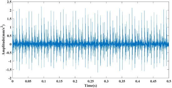
Figure 2.
Time domain diagram of the simulation signal.
Figure 3 presents the decomposition results of three types of signal decomposition methods. CEEMDAN decomposes signals into 13 modal components, which is far more than the ITD and ICEITDAN methods that are proposed in this paper. The modal-aliasing problem occurs on IMF 5 and IMF 6, while ICEITDAN alleviates this problem effectively. To evaluate the performance of the proposed method, the orthogonality index is used to compare the three methods. If one of two or more event species changes, other aspects will not be affected. Therefore, the orthogonality index can be selected to judge the independence between the decomposition components and determine whether the high- and low-frequency signals are accurately decomposed in the decomposed signal. Reference [42] also shows that the smaller the orthogonality index is, the higher the decomposition accuracy is, and the better the effect of endpoint effect suppression is via many experiments. Therefore, it is feasible to select an orthogonality index to evaluate the effect of endpoint effect suppression. In the comparison process, three performance indicators are considered—namely, the orthogonality indicator, the root mean square error (RMSE), and the run time—to quantitatively evaluate the decomposition performances of the methods [43,44,45,46]. Theoretically, the mode components that are decomposed by ICEITDAN, ITD, and CEEMDAN should be completely orthogonal—namely, the orthogonality index should be equal to zero. However, due to errors and environmental interference, the orthogonality index cannot be zero [42]. Therefore, the smaller the orthogonality index in the analysis is, the more accurate the decomposition is. The orthogonality index is defined as:
where represents the -th mode component that is decomposed.
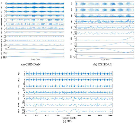
Figure 3.
Comparison chart of the decomposition results of three methods: Complete ensemble empirical mode decomposition with adaptive noise (CEEMDAN), improved complete ensemble intrinsic time-scale with adaptive noise (ICEITDAN), and intrinsic time decomposition (ITD). (a) CEEMDAN, (b) ICEITDAN, and (c) ITD.
The root mean square error (RMSE) is the square root of the ratio of the sum of squares of the deviation between the observed value and the true value to the number of observations m. It is used to measure the deviation between observed values and true values and judge the standard error between the decomposed signal and the original signal; also, it is used to represent dependency or decoupling. The run time parameter can be used to judge arithmetic efficiency. Therefore, the closer these three indicators are to 0, the higher their performance in signal processing. According to Table 1, the root mean square error and orthogonality index are the smallest and the closest to zero for the method that is proposed in this paper. In terms of run time, the method that is proposed in this paper requires less time than CEEMDAN but more than ITD. However, in contrast to the other two parameters and the signal reconstruction error of the ITD algorithm, the method that is proposed in this paper has a longer run time, but a higher precision. During practical use, the efficiency of the calculation will not be affected. The reason for the shorter computing time of ITD compared with the CEEMDAN method is that the core of the CEEMDAN method is the EMD algorithm. Compared with the EMD method, the ITD method avoids laborious and inefficient screening and spline interpolation processes and can decompose the original signal into A series of rotating components with a reliable instantaneous frequency and amplitude and residual monotonic trend signals, so the ITD method has the advantage of high computational efficiency. At the same time, the CEEMDAN method adds a group of white noise to the EMD method for decomposition. The CEEMDAN method calculates that the time was further extended. Compared with the ICEITDAN method, the ITD method performs a process of adding white noise in groups to improve the modal aliasing. Therefore, the ICEITDAN operation time is extended. Therefore, the method that is proposed in this paper is more suitable for practical engineering applications according to this comprehensive evaluation. In addition, according to the reconstruction error in Figure 4, the reconstruction error of the method that is proposed in this paper is the smallest among those of the three methods, and the peak value is less than , which can be regarded as the calculation error of the computer.

Table 1.
Comparison indicators for the three methods.
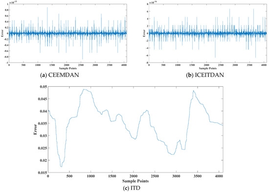
Figure 4.
Comparison of the reconstruction errors of three methods: CEEMDAN, ICEITDAN, and ITD. (a) CEEMDAN, (b) ICEITDAN, and (c) ITD.
Since signal decomposition is only used for noise reduction before fault feature extraction, it is necessary to select pattern components in the decomposition results for the extraction of the fault feature frequency. Kurtosis is a time domain parameter that is sensitive to faults, but kurtosis index pulse faults are sensitive, especially early faults, but not stable. Due to the use of the kurtosis as the component of the selected sensitive mode, it was found through the experiment that there was a deviation in the selected sensitive mode because non-Gaussian noise and a low signal-to-noise ratio more strongly influence the time domain kurtosis. With the objective of solving the problems of the signal selection and identification of fault-related sensitive mode components after processing, Wang and Shao [43] proposed an improved standard that was based on the periodic modulation intensity (PMI) that was proposed by Zhao and Jia [44]. The standard is defined as the ratio of periodic modulation components to the generalized interference (PMGI). The PMGI standard can be expressed as follows:
According to the proposed PMGI guidelines, only the growth of can induce the growth of PMGI. The higher the energy of the periodic modulation component is, the closer the PMGI is to 1.
Therefore, in this paper, we select the mode components for which the PMGI value exceeds the average value for reconstruction and perform envelope spectrum transformation to evaluate the performance of the method that is proposed in this paper. The PMGI values of the three methods are presented in Table 2. The PMGI values of the first two modes exceed the average values in the CEEMDAN decomposition results, whereas only one mode component exceeds the average values in ITD and ICEITDAN. The envelope analysis method mainly forms the envelope spectrum by adopting the form of envelope detection of the signal. Its main strategy is to use the envelope spectrum peak of the signal to judge the type of fault. This method is also referred to as an envelope solution. Its main advantage is that it can demodulate the fault vibration signal in high-frequency wells and provide effective interference cancellation for subsequent studies [45]. Therefore, we must reconstruct the first two mode components for CEEMDAN, select the first mode component for ITD and ICEITDAN, and obtain envelope spectra for the three signals after reconstruction. The results are presented in Figure 5. Only six times can the frequency fault feature frequency be clearly identified using the CEEMDAN and ITD methods. However, the method that is proposed in this paper identifies more than ten fault frequency peaks. Moreover, the amplitude of the envelope spectrum that is obtained via the CEEMDAN method is much smaller than that obtained by the method that is proposed in this paper; thus, the method that is proposed in this paper outperforms the others in fault feature extraction.
Table 2.
PMGI values of different methods.
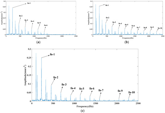
Figure 5.
Comparison chart of envelope spectrum results of the three methods: CEEMDAN, ICEITDAN, and ITD. (a) ITD, (b) ICEITDAN, and (c) CEEMDAN.
According to the comparison that is presented above, the ICEITDAN decomposition method that is proposed in this paper outperforms CEEMDAN and ITD. Therefore, in the next step, we will focus on the demodulation and analysis of ICEITDAN-CQMA for signals.
Based on the principles and results of the reconstruction of the sensitive mode components that are selected above, only the mode component GPR1 in this analog signal exceeds the mean PMGI value. Therefore, it is concluded that this mode component contains periodic pulse information; hence, GPR1 is selected as the main component for further analysis. With the objective of evaluating the performance of CQMA, the traditional demodulation method—namely, wavelet transform—and Teager–Kaiser energy operator (TKEO) are used to demodulate the reconstructed signal that is obtained through PMGI parameters after decomposition by the ICEITDAN method. The envelope spectrum of the obtained demodulation result is shown in Figure 6. By observing the fault frequency and harmonic wave in the three demodulation methods, it is found that fault feature frequency and the 16 harmonics behind it can be identified clearly in the frequency spectrum that has been demodulated by the CQMA method. However, the fault feature frequency and the harmonic wave are not easy to identify in the spectra that are obtained using wavelet transform and the TKEO method; thus, the method that is proposed in this paper outperforms the others in terms of signal demodulation.
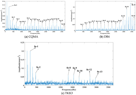
Figure 6.
Comparison chart of the envelope spectrum results of the composite quantum morphology analysis (CQMA), DB4, and Teager–Kaiser energy operator (TKEO) methods: (a) CQMA, (b) DB4 wavelet, and (c) TKEO.
To further evaluate the performance of the proposed CQMA method, we use the characteristic frequency intensity value as an index [43], and the feature frequency intensity coefficient represents the apparent degree of the frequency amplitude of the fault feature in the spectrogram. It is defined as follows:
where is the characteristic frequency intensity coefficient, is the amplitude value that corresponds to the fault feature frequency and the frequency doubling of the rolling bearing, and is the amplitude value of all frequencies in the envelope spectrum graph.
The characteristic frequency intensity value reflects the frequency ratio of the fault feature frequency in the spectrum diagram and reflects the effects of signal decomposition. The larger is, the better the signal decomposition effect and the more clearly the effects on the fault type are reflected in the envelope spectrum. The fault of bearings during diagnosis is unknown in practice. All faults of the bearing inner ring, outer ring, and rolling element must be calculated in advance. At this point, the characteristic frequency intensity coefficient is the ratio of the sum of the amplitudes that correspond to each fault and its frequency doubling to the sum of all frequency amplitudes. Therefore, as presented in Table 3, the characteristic frequency intensity value for the method that is proposed in this paper is maximal, which further demonstrates the effectiveness of this method in signal demodulation.
Table 3.
Characteristic frequency intensity values.
3.2. Experimental Studies
- (1)
- Experimental platform
A functional schematic diagram of the test platform is shown in Figure 7. Bearings 5 and 6 are tested bearings, and 4 and 7 are test bearings. The test bench uses an electric spindle as the driving force. The speed can be adjusted continuously, and the speed error does not exceed ±1%. During the experiment, the electric spindle rotates and loads bearings 5 and 6 (the loading capacity is 0~500 kg, and the loading accuracy is ±2%) to simulate the working environment of the bearing, while temperature sensor 3 collects the outside temperature of the bearing in real-time. Vibration sensors 10 and 11 collect the vibration acceleration signals of the tested bearing in real-time and transmit them to the acquisition card.
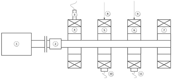
Figure 7.
Functional schematic diagram of the test platform. 1—electric spindle; 2—coupling; 3—temperature sensor; 4—accompanying bearing; 5—subject bearing; 6—subject bearing; 7—accompanying bearing; 8 and 9—loading system; 10 and 11—accelerometer.
The experimental platform consists of an experimental platform and a control system. Figure 8 shows a physical diagram of the experimental station, which consists mainly of a tested bearing, companion test bearing, test spindle, bearing outer ring fixture, drive unit, and loading system.
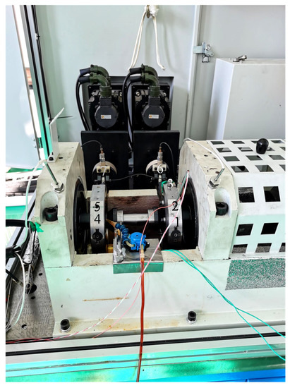
Figure 8.
Physical diagram of the experimental station. 1 and 2—tested bearing and its outer ring fixture; 3—vibration sensor; 4 and 5—companion test bearing and its outer ring fixture; 6 and 7—loading system.
Four sets of bearings, which included two sets of tested bearings and two sets of companion test bearings for a group, were used during the test. Two sets of loading systems were applied to the tested bearings. The drive unit provided power for the whole experimental platform and provided radial force for the tested bearing via the loading system; thus, the spindle drove the bearing to rotate, and the vibration signal of the bearing was obtained through the vibration sensor. The range of bearing speeds that the drive unit could provide was 1000 rpm~20,000 rpm, and the bearing speed was continuously adjustable. The loading range of the loading system was 0~6 KN, and the loading accuracy was and continuously adjustable. Since this test bench was a horizontal test bench, the sensor was placed above the bearing seat in the direction perpendicular to the ground and located in the Z axis direction of the bearing. This experimental acquisition system is a non-invasive acquisition system.
Figure 9 shows the fault diagram of the inner ring of the experimental bearing. It can be seen that there are only initial traces caused by the friction of the rolling elements, and there are no faults, such as cracks, which belong to the category of early faults. In Table 4 and Table 5, we present the test bearing parameters and the bearing failure characteristic frequency calculation formulas, respectively.
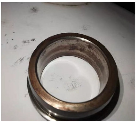
Figure 9.
Failure diagram of the experimental bearing inner ring.
Table 4.
Bearing parameters.
Table 5.
Bearing failure characteristic frequency calculation formulas.
The sampling frequency was 8192 Hz, and the data length was 4096 points. The bearing rotation speed was 3000 rpm. Based on Table 4 and Table 5, the fault feature frequencies of the inner ring were calculated as 407 Hz, and in the envelope spectrum, the fault feature frequencies of the inner ring and outer ring were , , , , and .
- (2)
- Analysis of the experimental results and discussion
Figure 10 presents the decomposition results of three types of signal decomposition methods, wherein CEEMDAN decomposes signals into 11 modal components, which is many more than ITD, and CEEMDAN has two more mode components than the proposed ICEITDAN method. In addition, modal aliasing occurs in IMF5 (intrinsic mode function) and IMF6, whereas ICEITDAN alleviates this problem well. To further evaluate the performance of the method that is proposed in this paper, the orthogonality index is used to compare the three methods. As presented in Table 6, the orthogonality index of the method that is proposed in this paper is minimal; hence, the decomposition performance of this method has been improved effectively compared with that of CEEMDAN and ITD. Figure 11 shows the reconstructed error after signal decomposition. The reconstruction error of the method that is proposed in this paper is smaller than that of the other two methods; hence, the method that is proposed in this paper has a higher decomposition precision than the other methods. Similarly, we calculate the root mean square error (RMSE) and computation time of each of the three methods and present the results in Table 6. The obtained parameter values show that the method that is proposed in this paper has substantial advantages over the other two methods.
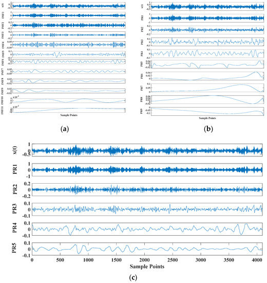
Figure 10.
Comparison chart of the decomposition results of three methods: CEEMDAN, ICEITDAN, and ITD. (a) CEEMDAN, (b) ICEITDAN, and (c) ITD.
Table 6.
Comparison indicators for the three methods.
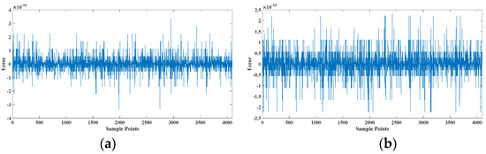

Figure 11.
Comparison of the reconstruction errors of three methods: CEEMDAN, ICEITDAN, and ITD. (a) CEEMDAN, (b) ICEITDAN, and (c) ITD.
Next, PMGI values are calculated for each mode component, and mode components that exceed the average values for reconstruction and envelope spectrum conversion are selected for use in extracting fault feature frequencies and identifying frequency doubling; the result is shown in Figure 12. By adopting the CEEMDAN and ITD methods, only four harmonics of the fault feature frequency can be clearly identified. The method that is proposed in this paper yields two more peaks of the fault feature frequency compared with these two methods. Therefore, the proposed method outperforms the others in terms of practical fault feature extraction.
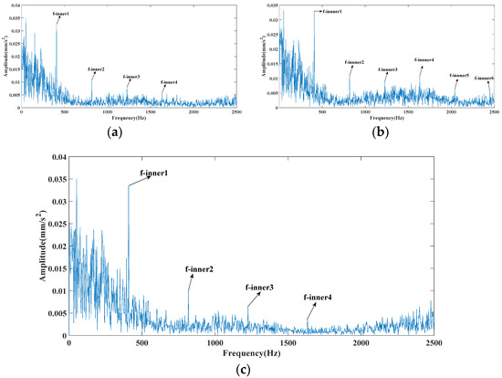
Figure 12.
Comparison chart of the envelope spectrum results of three methods: CEEMDAN, ICEITDAN, and ITD. (a) ITD, (b) ICEITDAN, and (c) CEEMDAN.
The envelope spectrum of the ICEITDAN results still contains strong noise, but the method that is proposed in this paper can effectively detect the early failure of the bearing inner ring. The reason is that the white noise that is added in the CEITDAN method can only be used to offset the white noise part of the signal, and the noise reduction in colored noise remains insufficient. This also verifies the packet that was extracted from the analog signal with only white noise added. The network spectrum does not contain noise interference. In addition, to better extract fault features, we must use the CQMA method for further analysis and demodulation. When extracting the fault feature frequency after decomposition, the CQMA method that is proposed in this paper can extract more fault feature frequencies of bearings than ICEITDAN, which explains the reliability, necessity, and foresight of the method that is proposed in this paper. In the envelope spectrum after CQMA demodulation, the influence of noise is reduced; thus, the technical solution that is proposed in this article can effectively solve the problem of difficult feature frequency extraction, due to excessive noise in the early failure and reduce noise better than the other methods.
According to the comparison above, the proposed ICEITDAN decomposition method outperforms CEEMDAN and ITD. Therefore, in the next step, we will focus on the demodulation and analysis of ICEITDAN-CQMA on signals. As presented earlier in Table 7, there are three mode components that exceed the mean PMGI value for the method that is proposed in this paper; hence, they are selected as signals for further analysis, and the signal is also reconstructed. To evaluate the performance of CQMA, wavelet transform is selected similarly, and the Teager–Kaiser energy operator (TKEO) is used to demodulate the reconstructed mode components that are obtained from the ICEITDAN method. The obtained demodulation results and their envelope spectra are shown in Figure 13. According to (a), the method that is proposed in this paper can clearly identify the fault frequency of the inner rolling bearing and its 7th frequency. However, the wavelet analysis in (b) shows that the fault frequency of the bearing cone and its 5th frequency are completely covered by noise and cannot be obtained. The envelope spectrum effect analysis by TKEO in (c) outperforms the wavelet analysis. However, its 7th fault frequency was covered by noise. Therefore, the fault diagnosis results of the proposed method are the same as those of the analog signal. To evaluate the performance of the release method that is proposed in this article, an experiment was also conducted on the outer ring fault. Due to space limitations, this article only presents the envelope spectrum result of the outer ring fault. Figure 12 shows that the proposed method can accurately locate the outer ring and the characteristic frequency of loop failure. At the same time, it maintains a high superiority and practicality. Therefore, the proposed CQMA method outperforms the commonly used wavelet and Teager–Kaiser energy operator methods. The proposed CQMA method has higher bearing fault feature frequencies than ICEITDAN, which also demonstrates the superior performance and necessity of the proposed CQMA algorithm.
Table 7.
PMGI values of different methods.
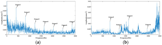
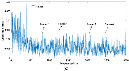
Figure 13.
Comparison chart of the envelope spectrum results of three methods: CQMA, DB4, and TKEO. (a) CQMA, (b) DB4 wavelet, and (c) TKEO.
To evaluate the performance of the proposed CQMA method in practical application, the results of the three methods are compared using the characteristic frequency intensity coefficient index in actual operation. As shown in Table 8, the characteristic frequency intensity of the CQMA method is the largest. This also shows from another angle that the method can effectively diagnose the early weak fault of the bearing. According to previous studies, when the rolling body passes through local defects, its time domain acceleration signal will produce a double-pulse phenomenon [42]. The reason for this is that when the rolling body passes through a local defect, a double pulse will be excited. Moreover, the larger the local defect, the greater the signal amplitude. Compared with the uniform inner and outer ring distribution, the fundamental frequency of the bearing vibration acceleration response is the same under the non-uniform distribution, while the amplitude and peak frequency increase.
Table 8.
Characteristic frequency intensity values.
To sum up, the proposed ICEITDAN-CQMA method not only achieves better results than the other methods in the feature extraction of analog signals, but also maintains the best results in the measured signals. This method has the advantages of small reconstruction error, low root mean square error, minimum orthogonality, shortest calculation time, and better extraction of feature frequency. It provides a good foundation for subsequent bearing fault diagnoses.
4. Conclusions
This paper proposes a feasible solution to the problems of modal aliasing, curve distortion, and end effects in a commonly used signal processing algorithm, ITD. Then, the paper applies the solution to the diagnosis of rolling bearings. In addition, the CQMA algorithm proposed in this paper applies quantum theory to triangular structural elements in a mathematical morphological analysis. The performance of the proposed ICEITDAN-CQMA method on simulation and experimental vibration signals is proven.
This study shows that the proposed method can successfully detect the fault frequency of rolling bearings. The main innovation of this paper is that the proposed envelope fitting method can effectively solve the problems of curve distortions and end effects that are caused by the traditional ITD method. According to a comparison of the commonly used wavelet analysis and Teager energy operator analysis methods, this method has stronger practicability. This is important for increasing the detection accuracy of early faults in rolling bearings.
Author Contributions
Conceptualization, J.M.; methodology, J.M.; software, G.-Z.Z.; validation, J.M., L.Z.; formal analysis, G.C.; investigation, J.M.; resources, L.Z.; data curation, J.M.; writing—original draft preparation, J.M.; writing—review and editing, L.Z. and C.L.; visualization, C.L.; supervision, C.L.; project administration, CL. All authors have read and agreed to the published version of the manuscript.
Funding
This research received no external funding.
Institutional Review Board Statement
Not applicable.
Informed Consent Statement
Not applicable.
Data Availability Statement
Not applicable.
Conflicts of Interest
The authors declare no conflict of interest.
References
- Tong, Q.; Cao, J.; Han, B.; Zhang, X.; Nie, Z.; Wang, J.; Lin, Y.; Zhang, W. A fault diagnosis approach for rolling element bearings based on RSGWPT-LCD bilayer screening and extreme learning machine. IEEE Access 2017, 5, 5515–5530. [Google Scholar] [CrossRef]
- Yu, J.; Lv, J. Weak fault feature extraction of rolling bearings using local mean decomposition-based multilayer hybrid denoising. IEEE Trans. Instrum. Meas. 2017, 66, 3148–3159. [Google Scholar] [CrossRef]
- Li, H.; Li, Z.; Mo, W. A time varying filter approach for empirical mode decomposition. Signal Process. 2017, 138, 146–158. [Google Scholar] [CrossRef]
- Zhang, Y.; Du, X.; Wen, G.; Huang, X.; Zhang, Z.; Xu, B. An adaptive method based on fractional empirical wavelet transform and its application in rotating machinery fault diagnosis. Meas. Sci. Technol. 2018, 30, 035005. [Google Scholar] [CrossRef]
- Qiao, Z.; Pan, Z. SVD principle analysis and fault diagnosis for bearings based on the correlation coefficient. Meas. Sci. Technol. 2015, 26, 085014. [Google Scholar] [CrossRef]
- Qiao, Z.; Lei, Y.; Li, N. Applications of stochastic resonance to machinery fault detection: A review and tutorial. Mech. Syst. Signal Process. 2019, 122, 502–536. [Google Scholar] [CrossRef]
- Khalil, K.; Eldash, O.; Kumar, A.; Bayoumi, M. Intelligent fault-prediction assisted self-healing for embryonic hardware. IEEE Trans. Biomed. Circuits Syst. 2020, 14, 852–866. [Google Scholar] [CrossRef]
- Khalil, K.; Eldash, O.; Kumar, A.; Bayoumi, M. Machine learning-based approach for hardware faults prediction. IEEE Trans. Circuits Syst. I Regul. Pap. 2020, 67, 3880–3892. [Google Scholar] [CrossRef]
- Razavi-Far, R.; Hallaji, E.; Farajzadeh-Zanjani, M.; Saif, M.; Kia, S.H.; Henao, H.; Capolino, G.A. Information Fusion and Semi-Supervised Deep Learning Scheme for Diagnosing Gear Faults in Induction Machine Systems. IEEE Trans. Ind. Electron. 2019, 66, 6331–6342. [Google Scholar] [CrossRef]
- Razavi-Far, R.; Hallaji, E.; Saif, M.; Ditzler, G. A Novelty Detector and Extreme Verification Latency Model for Nonstationary Environments. IEEE Trans. Ind. Electron. 2018, 66, 561–570. [Google Scholar] [CrossRef]
- Frei, M.G.; Osorio, I. Intrinsic time-scale decomposition: Time–frequency–energy analysis and real-time filtering of non-stationary signals. Proc. R. Soc. A Math. Phys. Eng. Sci. 2006, 463, 321–342. [Google Scholar] [CrossRef]
- Amirat, Y.; Choqueuse, V.; Benbouzid, M. EEMD-based wind turbine bearing failure detection using the generator stator current homopolar component. Mech. Syst. Signal Process. 2013. [Google Scholar] [CrossRef]
- Zhang, J.-H.; Liu, Y. Application of complete ensemble intrinsic time-scale decomposition and least-square SVM optimized using hybrid DE and PSO to fault diagnosis of diesel engines. Front. Inf. Technol. Electron. Eng. 2017, 18, 272–286. [Google Scholar] [CrossRef]
- Xing, Z.; Qu, J.; Chai, Y.; Tang, Q.; Zhou, Y. Gear fault diagnosis under variable conditions with intrinsic time-scale decomposition-singular value decomposition and support vector machine. J. Mech. Sci. Technol. 2017, 31, 545–553. [Google Scholar] [CrossRef]
- Xiang, L.; Hu, A.; Gao, N. Fault diagnosis for the gearbox of wind turbine combining ensemble intrinsic time-scale decomposition with Wigner bi-spectrum entropy. J. Vibroeng. 2017, 19, 1759–1770. [Google Scholar] [CrossRef]
- Liu, Y.; Zhang, J.; Qin, K.; Xu, Y. Diesel engine fault diagnosis using intrinsic time-scale decomposition and multistage Adaboost relevance vector machine. Proc. Inst. Mech. Eng. Part C J. Mech. Eng. Sci. 2017, 232, 881–894. [Google Scholar] [CrossRef]
- Bi, F.; Ma, T.; Liu, C.; Tian, C. Knock detection in spark ignition engines based on complementary ensemble improved intrinsic time-scale decomposition (CEIITD) and Bi-spectrum. J. Vibroeng. 2018, 20, 936–953. [Google Scholar] [CrossRef]
- Yu, J.; Liu, H. Sparse coding shrinkage in intrinsic time-scale decomposition for weak fault feature extraction of bearings. IEEE Trans. Instrum. Meas. 2018, 67, 1579–1592. [Google Scholar] [CrossRef]
- Liu, H.; Xiang, J. Kernel regression residual signal-based improved intrinsic time-scale decomposition for mechanical fault detection. Meas. Sci. Technol. 2018, 30, 015107. [Google Scholar] [CrossRef]
- Li, Z.; Li, Y.; Zhang, K. A feature extraction method of ship-radiated noise based on fluctuation-based dispersion entropy and intrinsic time-scale decomposition. Entropy 2019, 21, 693. [Google Scholar] [CrossRef] [PubMed]
- Yuan, Z.; Peng, T.; An, D.; Cristea, D.; Pop, M.A. Rolling bearing fault diagnosis based on adaptive smooth ITD and MF-DFA method. J. Low Freq. Noise, Vib. Act. Control. 2020, 39, 968–986. [Google Scholar] [CrossRef]
- Amirat, Y.; Benbouzid ME, H.; Wang, T.; Bacha, K.; Feld, G.J.A.A. EEMD-based notch filter for induction machine bearing faults detection. Appl. Acoust. 2018, 133, 202–209. [Google Scholar] [CrossRef]
- Hu, A.; Xiang, L. Selection principle of mathematical morphological operators in vibration signal processing. J. Vib. Control. 2014, 22, 3157–3168. [Google Scholar] [CrossRef]
- Dong, Y.; Liao, M.; Zhang, X.; Wang, F. Fault diagnosis of rolling element bearings based on modified morphological method. Mech. Syst. Signal Process. 2011, 25, 1276–1286. [Google Scholar] [CrossRef]
- Lv, J.; Yu, J. Average combination difference morphological filters for fault feature extraction of bearing. Mech. Syst. Signal Process. 2011, 25, 1276–1286. [Google Scholar] [CrossRef]
- Eldar, Y.C.; Oppenheim, A.V. Oppenheim, “Quantum signal processing”. IEEE Signal Process. Mag. 2002, 19, 12–32. [Google Scholar] [CrossRef]
- Cai, G.; Chen, X.; He, Z. Sparsity-enabled signal decomposition using tunable Q-factor wavelet transform for fault feature extraction of gearbox. Mech. Syst. Signal Process. 2013, 41, 34–53. [Google Scholar] [CrossRef]
- Rodríguez, P.H.; Alonso, J.B.; Ferrer, M.A.; Travieso, C.M. Application of the Teager–Kaiser energy operator in bearing fault diagnosis. ISA Trans. 2013, 52, 278–284. [Google Scholar] [CrossRef]
- Chen, Q.; Huang, N.; Riemenschneider, S.D.; Xu, Y. A B-spline approach for empirical mode decompositions. Adv. Comput. Math. 2006, 24, 171–195. [Google Scholar] [CrossRef]
- Fan, Z.P.; Hong, T.S.; Liu, Z.Z.; Jing, Z.Z. Improve the envelope of EMD with piecewise linear fractal interpolation. Key Eng. Mater. 2010, 439-440, 390–395. [Google Scholar] [CrossRef]
- Zhu, W.; Zhao, H.; Chen, X. Improving empirical mode decomposition with an optimized piecewise cubic Hermite interpolation method. In Proceedings of the 2012 International Conference on Systems and Informatics (ICSAI2012), Yantai, China, 19–20 May 2012; pp. 1698–1701. [Google Scholar]
- Li, Y.; Xu, M.; Liang, X.; Huang, W. Application of bandwidth EMD and adaptive multiscale morphology analysis for incipient fault diagnosis of rolling bearings. IEEE Trans. Ind. Electron. 2017, 64, 6506–6517. [Google Scholar] [CrossRef]
- Fu, X.-W.; Ding, M.-Y.; Cai, C. Despeckling of medical ultrasound images based on quantum-inspired adaptive threshold. Electron. Lett. 2010, 46, 889–891. [Google Scholar] [CrossRef]
- Ma, J.; Zhan, L.; Li, C.; Li, Z. An improved intrinsic time-scale decomposition method based on adaptive noise and its application in bearing fault feature extraction. Meas. Sci. Technol. 2020, 32, 025103. [Google Scholar] [CrossRef]
- HLi, H.; Xiao, D.-Y. Fault diagnosis using pattern classification based on one-dimensional adaptive rank-order morphological filter. J. Process. Control. 2012, 22, 436–449. [Google Scholar] [CrossRef]
- Lv, C.; Zhang, P.; Wu, D.; Li, B.; Zhang, Y. Bearing fault signal analysis based on an adaptive multiscale combined morphological filter. Int. J. Rotating Mach. 2020, 7567439, 8. [Google Scholar] [CrossRef]
- Zhang, L.; Xu, J.; Yang, J.; Yang, D.; Wang, D. Multiscale morphology analysis and its application to fault diagnosis. Mech. Syst. Signal Process. 2008, 22, 597–610. [Google Scholar] [CrossRef]
- Yuan, S.; Mao, X.; Chen, L.; Xue, Y. Quantum digital image processing algorithms based on quantum measurement. Optik 2013, 124, 6386–6390. [Google Scholar] [CrossRef]
- Kiranyaz, Ç.S.; Gabbouj, M. Quantum mechanics in computer vision: Automatic object extraction. In Proceedings of the 2013 IEEE International Conference on Processing, Melbourne, Australia, 15–19 September 2013; pp. 2489–2493. [Google Scholar]
- Nikolaou, N.; Antoniadis, I. Application of morphological operators as envelope extractors for impulsive-type periodic signals. Mech. Syst. Signal Process. 2003, 17, 1147–1162. [Google Scholar] [CrossRef]
- Torres, M.E.; Colominas, M.A.; Schlotthauer, G.; Flandrin, P. A complete ensemble empirical mode decomposition with adaptive noise. In Proceedings of the 2011 IEEE International Conference on Acoustics, Speech and Signal Processing (ICASSP), Prague, Czech Republic, 22–27 May 2011; pp. 4144–4147. [Google Scholar]
- Li, H.Y.; Wang, Z.L.; Zhen, D.; Gu, F.S.; Ball, A. Modulation Sideband separation using the Teager-Kaiser Energy Operator for Rotor Fault Diagnostics of Induction Moters. Energies 2020, 23, 4437. [Google Scholar]
- Wang, L.; Shao, Y. Fault feature extraction of rotating machinery using a reweighted complete ensemble empirical mode decomposition with adaptive noise and demodulation analysis. Mech. Syst. Signal Process. 2020, 138, 106545. [Google Scholar] [CrossRef]
- Zhao, M.; Jia, X. A novel strategy for signal denoising using reweighted SVD and its applications to weak fault feature enhancement of rotating machinery. Mech. Syst. Signal Process. 2017, 94, 129–147. [Google Scholar] [CrossRef]
- Yang, Y.; He, Y.; Cheng, J.; Yu, D. A gear fault diagnosis using Hilbert spectrum based on MODWPT and a comparison with EMD approach. Measurement 2009, 42, 542–551. [Google Scholar] [CrossRef]
- Desquilbet, L.; Mariotti, F. Dose-response analyses using restricted cubic spline functions in public health research. Stat. Med. 2010, 29, 1037–1057. [Google Scholar] [CrossRef] [PubMed]
Publisher’s Note: MDPI stays neutral with regard to jurisdictional claims in published maps and institutional affiliations. |
© 2021 by the authors. Licensee MDPI, Basel, Switzerland. This article is an open access article distributed under the terms and conditions of the Creative Commons Attribution (CC BY) license (http://creativecommons.org/licenses/by/4.0/).