3D Roughness Measurement of Failure Surface in CFA Pile Samples Using Three-Dimensional Laser Scanning

Abstract

The bearing capacity of CFA (Continuous Flight Auger) pile is not able to reach the design capacity if proper construction is not performed due to the soil collapse at the bottom of the pile. In this paper, three pile samples were prepared to simulate the bottom of the CFA pile: grouting sample; mixture of grouting and gravel; mixture of grouting and sand. The failure surfaces of each sample obtained by a uniaxial compression tests were represented as a three-dimensional point cloud by three-dimensional laser scanning. Therefore, high resolution of point clouds can be obtained to simulate the failure surfaces of three samples. The three-dimensional point cloud of each failure surface was analyzed by a plane to points histogram (P2PH) method and a roughness detection method by kernel proposed in this paper. These methods can analyze the global roughness as well as the local roughness of the three pile samples in three dimensions. The roughness features of the grouting sample, the mixed sample of grouting and sand, and the mixed sample of grouting and gravel can be distinguished by the sections where points of each sample are predominantly distributed in the histogram of the proposed method.

1. Introduction

The CFA (Continuous Flight Auger) pile has been widely used in recent years on ground where soil collapse can occur in the borehole due to the groundwater flow. In the CFA pile construction, the grouting is injected direct after excavation of a borehole in the CFA pile and hence the soil collapse can be minimized by confining of grouting in the borehole. Since the CFA pile is mainly constructed on weak ground conditions, studies have been conducted to estimate the bearing capacity and the behavior of CFA piles in various grounds (Farrell and Lawler, 2008, Gavin et al., 2009, Battista et al., 2016, Loveridge and Cecinato, 2016 [1,2,3,4,5,6,7,8,9,10]). In the CFA pile, the loss of ground can affect the bearing capacity of the pile (Leznicki et al., 1992 [8]). Seo (2020) [11,12,13,14] conducted a pile test on the CFA pile, and the main purpose of the loading test of the CFA pile was to evaluate the strength of the pile induced by the collapse of the soil. Therefore, this paper determined the behavior of the bottom of the pile affected by the soil collapse in the borehole along with the extension of this study. In particular, the roughness of the failure surface was evaluated with pile samples that simulate mixtures of grouting and soils at the bottom of the CFA pile.

Studies have been conducted to measure roughness in geotechnical engineering. The shear strength between soil and structure is also affected by the roughness (Seo et al. (2012), Seo et al. (2014) [15,16]) Therefore, it was considered in the design of structure and development of geotechnical structure (Seo et al. (2017), Seo et al. (2019) [17,18]). Lee and Juang (1991) [7] measured the roughness profile of rock joints using a laser displacement meter (LDM) and a linear variable differential transformer (LVDT). However, it was focused on measuring the roughness in one dimension. Hong et al. (2006) [6] proposed a new rock joint surface roughness measurement method by using a camera-type three-dimensional (3D) scanner as an alternative to previous methods. Tran et al. (2017) [19,20,21,22,23,24] developed a stereo photogrammetry computational program in which three-dimensional (3D) soil surface coordinates were derived from digital stereo pair images of soil samples following erosion tests. Li et al. (2018) [9] presented a spiral sampling method that addresses the shortcomings of the straight-line method. The roughness parameters derived from the spiral scanlines are closely correlated with the Joint Roughness Coefficient (JRC) values back-calculated from direct shear tests. Research to define the relation between measured roughness and the strength of the ground has been performed (Bauret and Rivard, 2018, Wang et al., 2019 [2,25]). Studies on the correlation between roughness and the bearing capacity of foundations such as piles have been also conducted (Tehrani et al., 2016, Sethy et al., 2018 [20,23]). Recently, SMART monitoring technologies have been applied to the various structures and studies to measure the roughness by using laser scanning have been conducted (Soga et al., 2015 [22]) Rauthause et al. (2019) [12] quantified surface roughness using laser scanning with application to the frictional resistance of sand–timber pile interfaces. Seo et al. (2019) [19] evaluated the displacement of rough structure during the excavation. Sobola et al. (2017) [21] applied atomic force microscopy (AFM) to define the features of wings scales of butterflies in microscale.

In this paper, the roughness of the failure surface obtained by compression testing mixed samples of grouting and soils simulating the bottom of a CFA pile is measured by terrestrial laser scanning. A plane to points histogram (P2PH) method and a roughness detection method by kernel were proposed in this paper to estimate the roughness of the failure surfaces in each pile sample. The proposed analysis methods can discriminate three-dimensional roughness of the failure surfaces in each pile sample, the global roughness as well as the local roughness of the failure surface can be estimated by the proposed method.

2. Test Materials

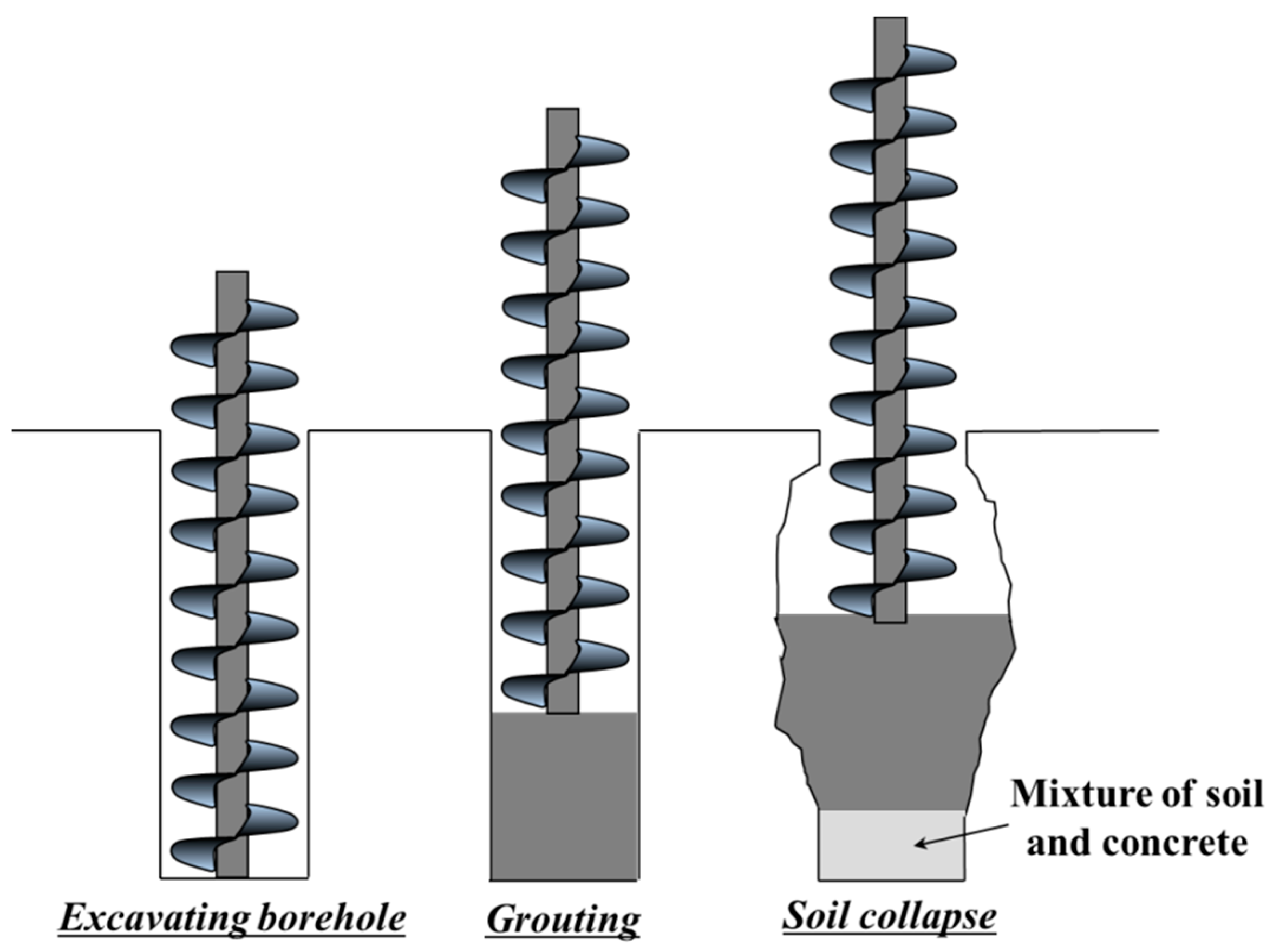
2.1. Ground Collapse in CFA Pile

When the ground is weak or groundwater condition, a borehole of the bored pile can be collapsed so that the bored pile is not appropriately constructed (Pelecanos et al. (2018), Battista et al. (2016) [1,11]). However, if the grouting is injected immediately after drilling the CFA pile, the soil collapse can be reduced. Therefore, it is possible to minimize the soil collapsing effect in conditions of weak ground or groundwater. Despite the application of the CFA pile, the ground in the borehole can be collapsed due to the inflow of groundwater. If the ground is deposited on the bottom of the pile due to the soil collapse, grouting can be mixed with collapsed soil during the concrete pouring as shown in Figure 1. Therefore, a bearing capacity is not only reached as much as the design load but local failure between the soil and grouting can also occur under the loading condition. The local failure is differently generated depending on the ground type. In this paper, samples of a mixture of ground and grouting were prepared to simulate the bottom of the CFA pile where the soil collapse can occur. Then, uniaxial compressive loading tests were conducted with these samples to collect failure surfaces of each pile sample. The failure behavior of the sample is affected by the roughness of the failure surface of the mixture, and the roughness of the failure surface is determined by the mixture type. Therefore, roughness estimation methods were proposed in this paper to analyze the roughness of the collected failure surface in three dimensions.

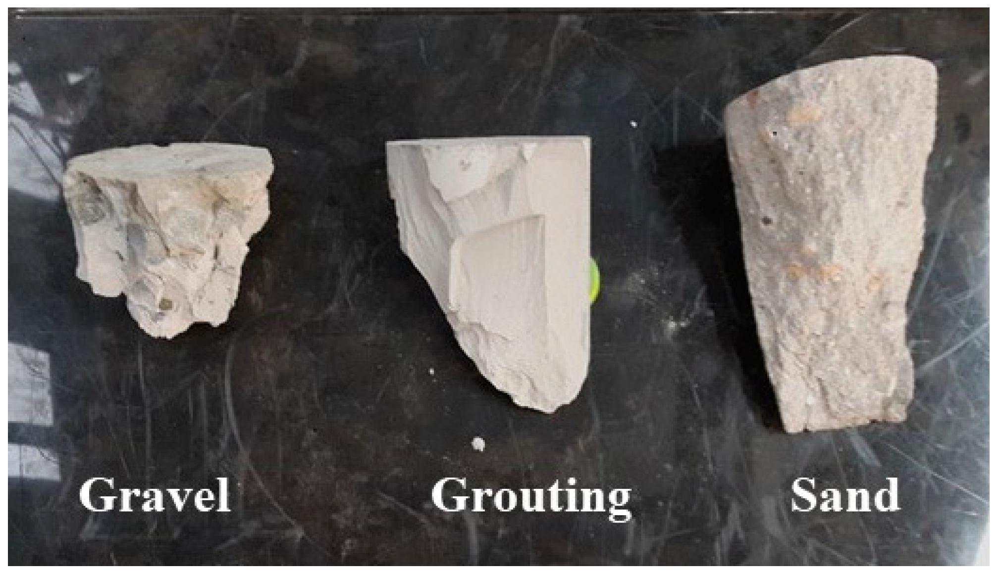
2.2. Uniaxial Compression Test to Obtain Failure Surfaces of CFA Pile Samples

In this paper, a grouting sample, a mixed sample of sand and grouting, and a mixed sample of gravel and grouting were prepared. The grouting sample means that there is no effect from the soil collapse into the borehole of the CFA pile. Sand sample and gravel sample were prepared with a ratio of grouting and both soils of 1:1. Three samples were prepared for each case, and a uniaxial compression test was performed with strain control. The purpose of this uniaxial compression test is to obtain a failure surface that can determine the roughness of each pile sample. Therefore, this paper focuses on estimating the three-dimensional roughness of the failure surface rather than the stress–strain relationship.

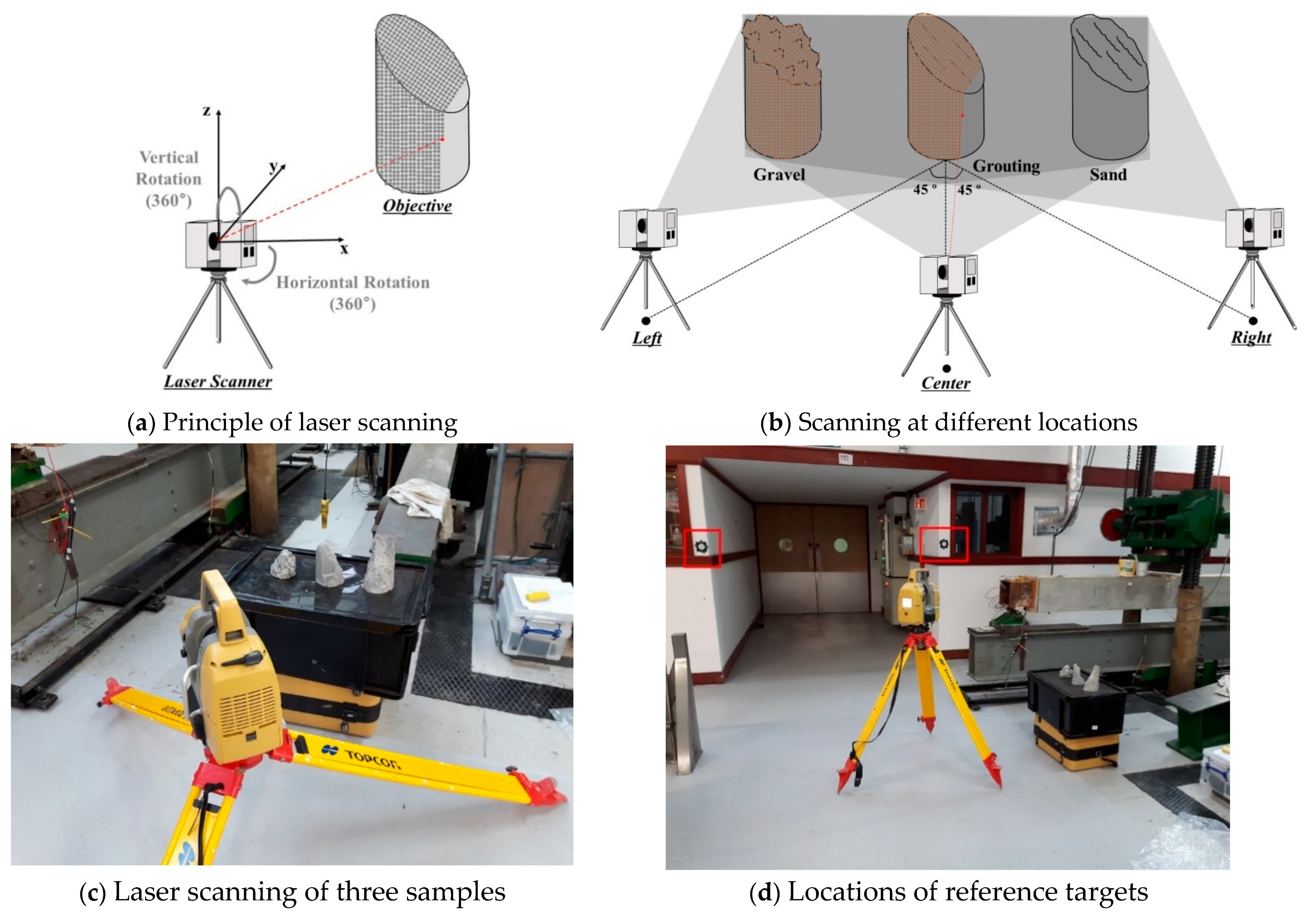
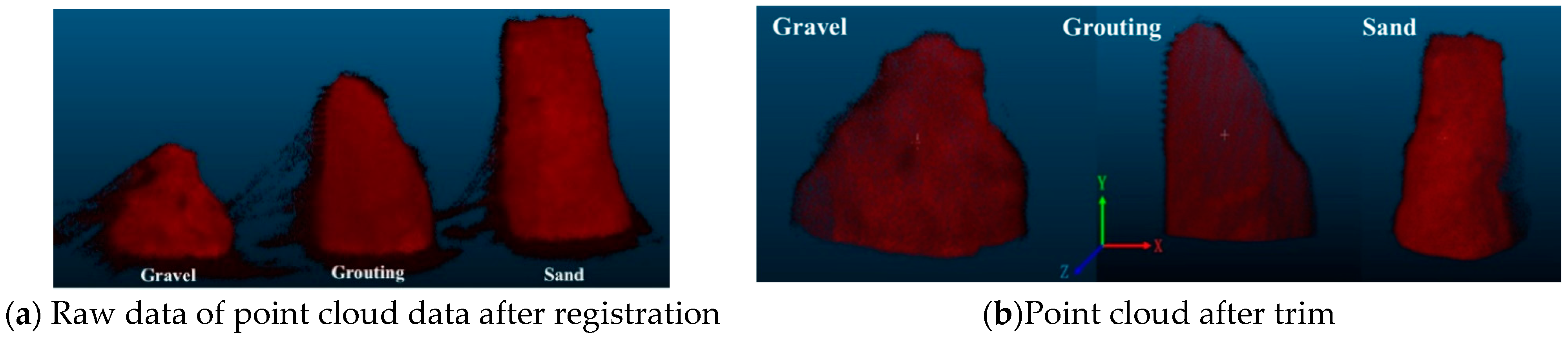
3. Test Method: 3D Laser Scanning

The collapsed samples were collected after uniaxial compression test. The roughness of the failure surface is different with the ground type mixed with concrete. If the soil particles size is large, the failure can occur at the boundary between the grouting and the soil. The shape of the failure surface is affected by the soil type and hence the failure surface was scanned to determine the roughness of the failure surface in three types of pile samples. The collapsed samples are grouting samples, mixed samples of grouting and gravel (100%), and mixed samples of grouting and sand (100%) (see Figure 2).

The technologies to simulate the three-dimensional shape of a structure are limited, such as a three-dimensional camera or three-dimensional laser scanning. The three-dimensional laser scanning has higher resolution and accuracy than other methods. Therefore, in order to measure local curvature such as roughness, 3D laser scanning with high resolution should be used. As shown in Figure 3a, the laser scanner can shoot lasers by rotating a laser head in the vertical and transverse directions and then collects reflected lasers from the object. The reflected point is expressed in three-dimensional coordinates by calculating the x, y, z positions of each point using the speed of the laser, the time of the reflected laser, and the angle of the laser scanner in the vertical and transverse directions. It is necessary to understand the local shape change of the failure surface to define the roughness. Especially, there are many areas affected by partial shadowing due to the gravel protrusion in the gravel sample and hence scanning was performed at three locations: center of the sample, and 45° away from the center (see Figure 3b). The laser scanning was performed by using TOPCON gls 2000 scanner as shown in Figure 3c. The resolution of the scanner was set as 3.1 mm when the distance between the scanner and the object is 10 m. The distance between the scanner and the pile samples was about 1 m so that the actual resolution is approximately 0.3 mm. Two scans were performed at the same location to increase resolution and accuracy. Since six laser scans were performed in total, it is expected to have six times higher resolution than the set resolution. The local coordinates of each scanning data can be changed by the different scanning locations. Target scanning was performed with three reference targets to merge different scanned point clouds into a same coordinate system, as shown in Figure 3d. Tilting of scanner was checked after the completion of the scanning to determine if there was movement of the laser scanner. There were angle changes before and after scanning which can be considered a negligible movement.

Figure 4 shows schematic diagrams of the expected point clouds of each sample at different scanning locations. Gravel sample is expected to have more shadowed effects. The overall roughness can be expressed by merging the point clouds collected at the front and sides due to the protrusion of gravels from the failure surface (see Figure 4a). Therefore, scanning at various angles is essential in gravel samples in order to evaluate the roughness appropriately. In the grouting sample, the resolution of point cloud of failure surface can be different depending on the scanning location. However, if there is a section in which the angle of the failure surface is changed sharply, this section can be expressed in more detail with multiple scanning at different locations (see Figure 4b). The grain size of sand is about 1 mm. Since the resolution of the laser scanning used in this paper is 0.3 mm and six scans were performed, the roughness caused by the sand grain can be detected on the failure surface of the sand sample. As shown in Figure 4c, the failure surface of the sand sample can be partially shaded by the locally curved area and the sand grain. Therefore, if point clouds are merged, not only an increase in resolution but also a local curvature can be detected.

Figure 5a shows the raw data of point clouds after the registration process that point clouds are merged into the same coordinate. Unnecessary point clouds in Figure 5a are trimmed for the roughness analysis, which is shown in Figure 5b.

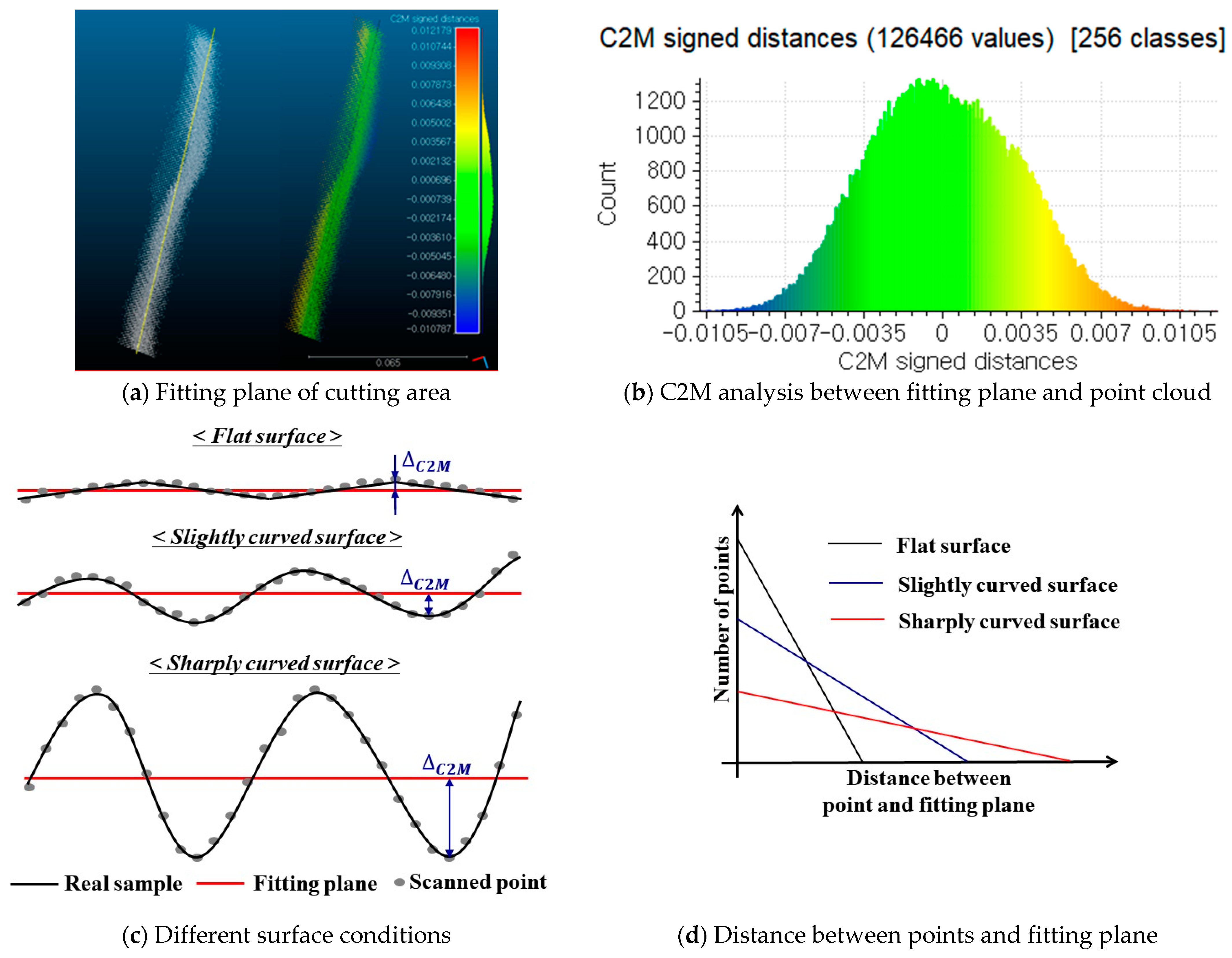
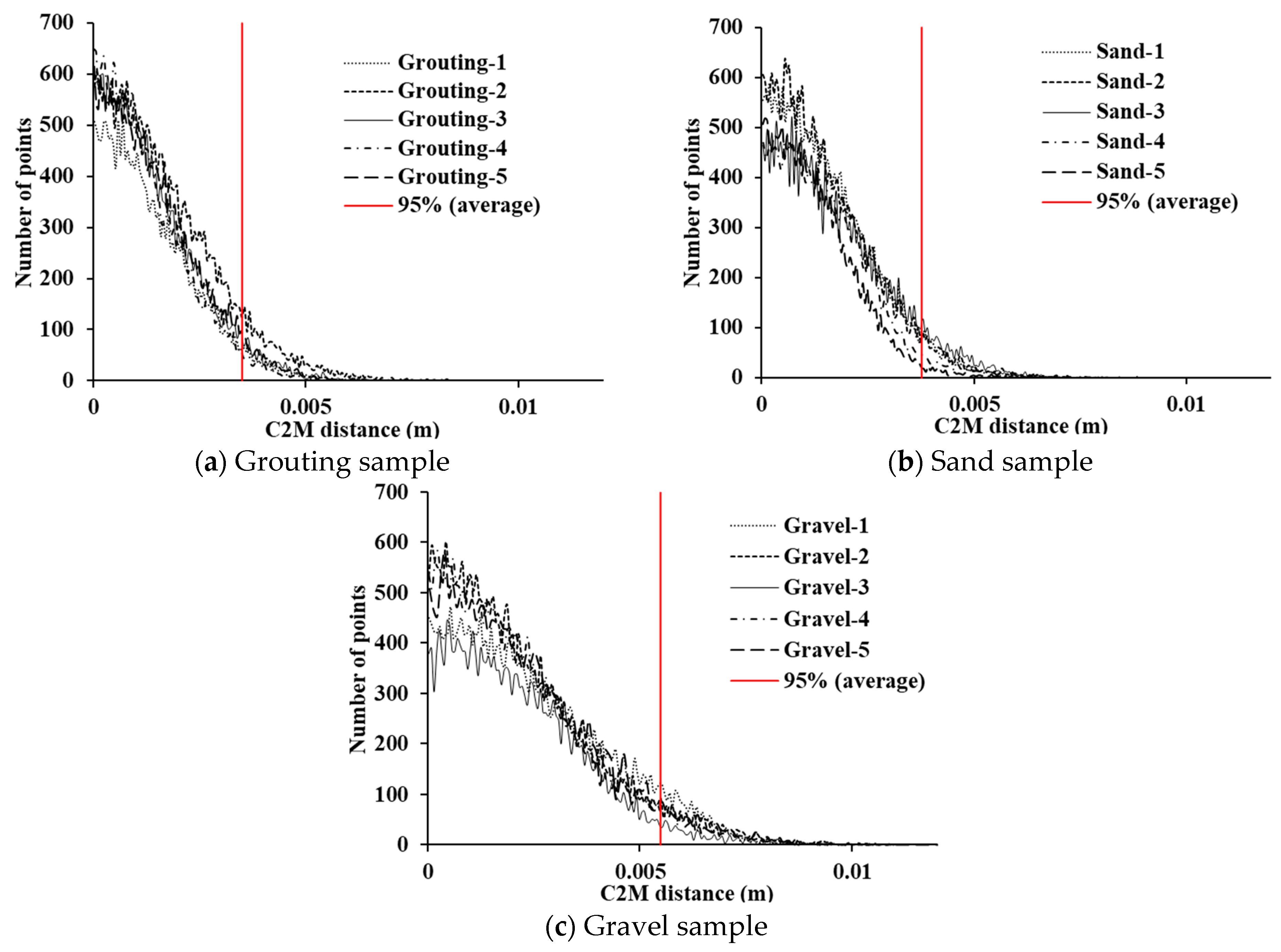
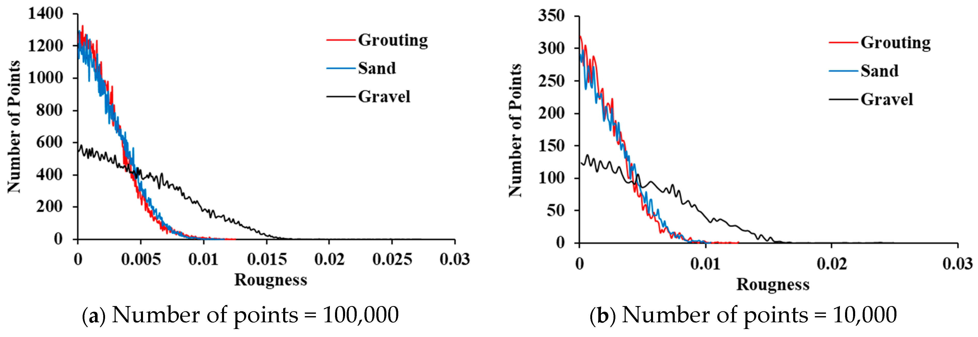
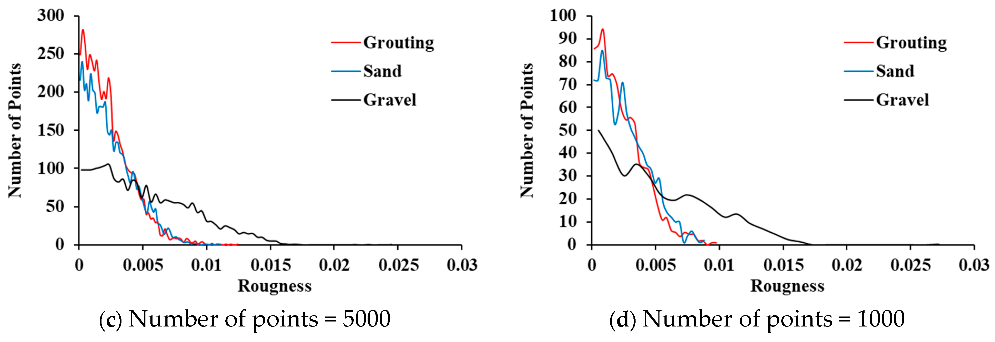
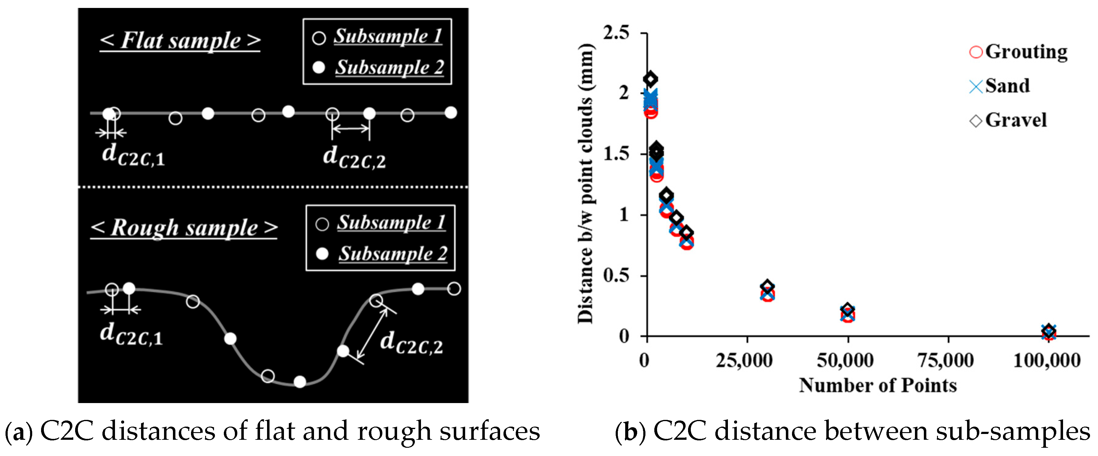
4. Analysis of Plane to Points Histogram (P2PH)

Various methods have been applied to determine the roughness of the failure surface of soils, but the roughness is expressed in one or two dimensions in most studies. However, the point cloud obtained from laser scanning is represented in three dimensions and hence this paper proposed a roughness measuring technique and assessment method to determine the roughness of failure surface.

4.1. Analysis Method

In order to determine the roughness of the three-dimensional point cloud, Plane to Points histogram (P2PH) method was proposed that a two-dimensional fitting plane representing the point cloud of the failure surface is compared with the points of the failure surface. In order to evaluate the roughness of the point cloud of each pile sample, the point cloud of the failure surface was cut into five parts with a rectangle. The size of the gravel is 20 mm so that the fitting plane size was set to 20 mm in width and 50 mm in length in order to reflect the curvature of the gravel in 3D roughness. If the size of the fitting plane becomes larger, the overall curvature is reflected in the analysis result rather than the roughness of the grouting or sand sample. The point cloud in cutting area can fit a plane which is closest to the point clouds among all planes that exist on three dimensions. It means that a rectangular mesh that is most similar to the shape of the cut point cloud can be obtained by calculating the average distance between a plane and points. The fitting plane can be a reference mesh for calculating the distance between the fitting plane and each point, as shown in Figure 6a. Since the fitting surface is recognized as a mesh, Cloud to Mesh (C2M) comparison method was used that calculates the distance between the point cloud and a fitting plane. Points close to the fitting plane are represented in blue, and points far from the fitting plane are represented in red. The distribution of points according to the C2M distance can be expressed as shown in Figure 6b. Figure 6c shows three cases of failure planes: flat failure surface, slightly curved failure surface, and severely curved failure surface. The C2M distance can be varied depending on the roughness of the failure surface. The point cloud of a flat failure surface is distributed close to a fitting plane. However, if the failure surface is rougher, the points are spread further from a fitting plane. Therefore, if the distance between points and a fitting plane is calculated by the C2M method, the C2M distance increases with the increase of roughness. Figure 6d shows a schematic diagram of the histogram of the expected C2M distance with different roughness. Most of the points are densely distributed at a small range of C2M distance in the flat failure surface. However, as the failure surface becomes rougher, the range of C2M distance can be wider. In this paper, the histogram was used as a criterion to assess the roughness, and the point cloud analysis of the failure surface of pile samples was conducted.

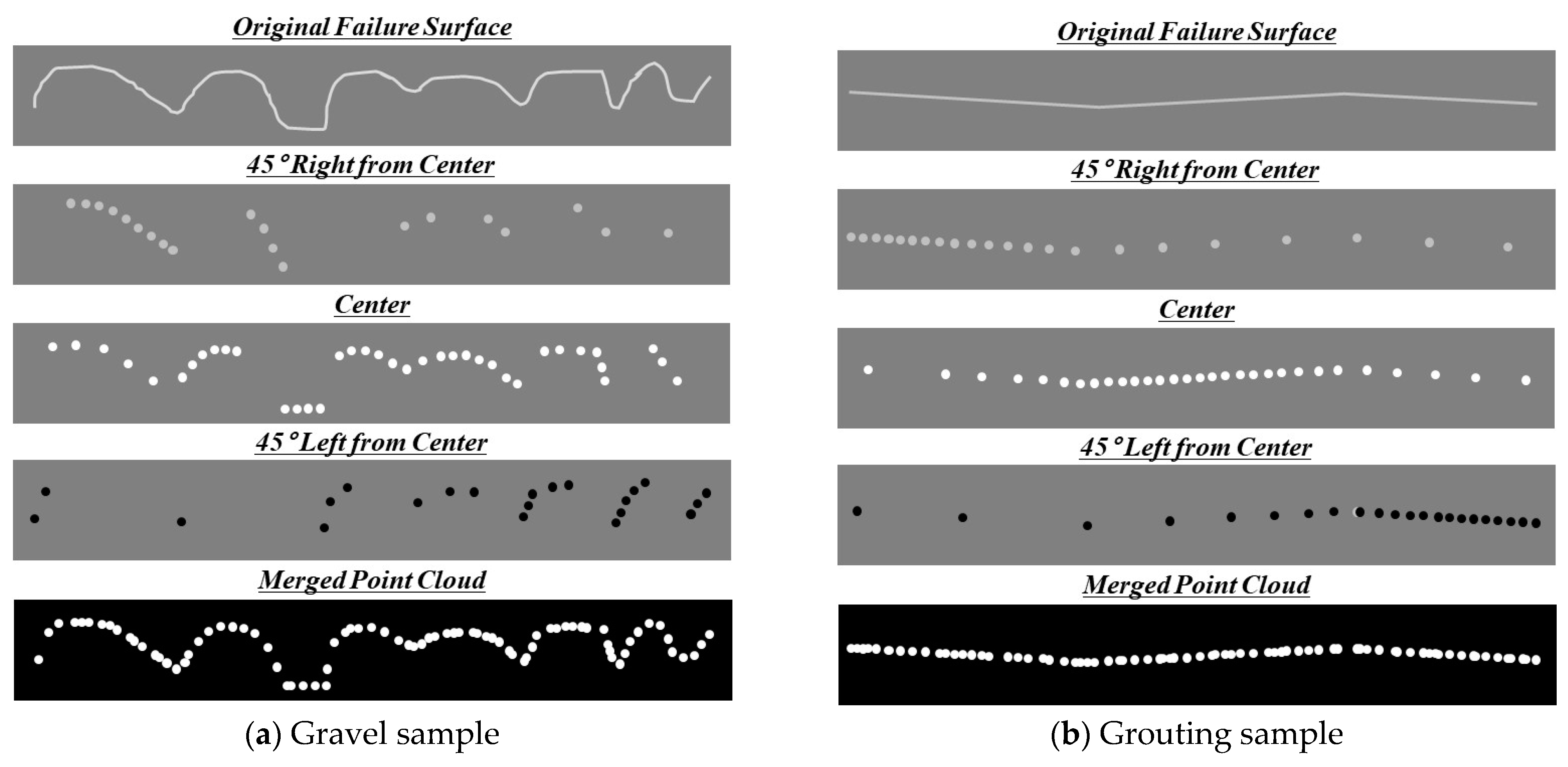
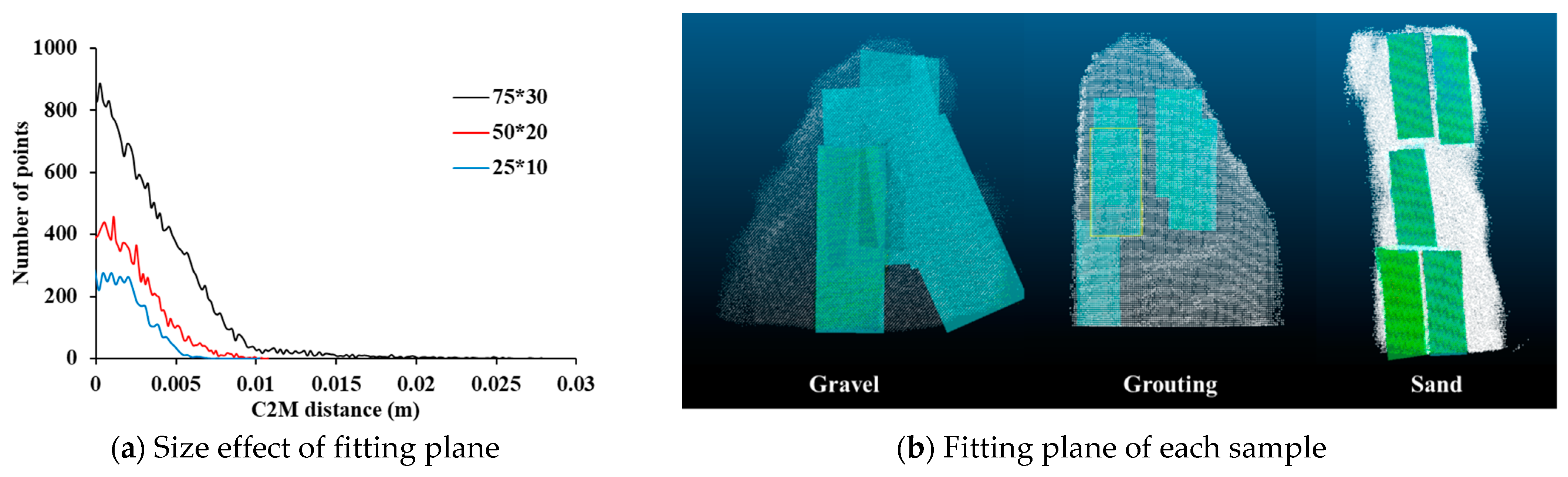
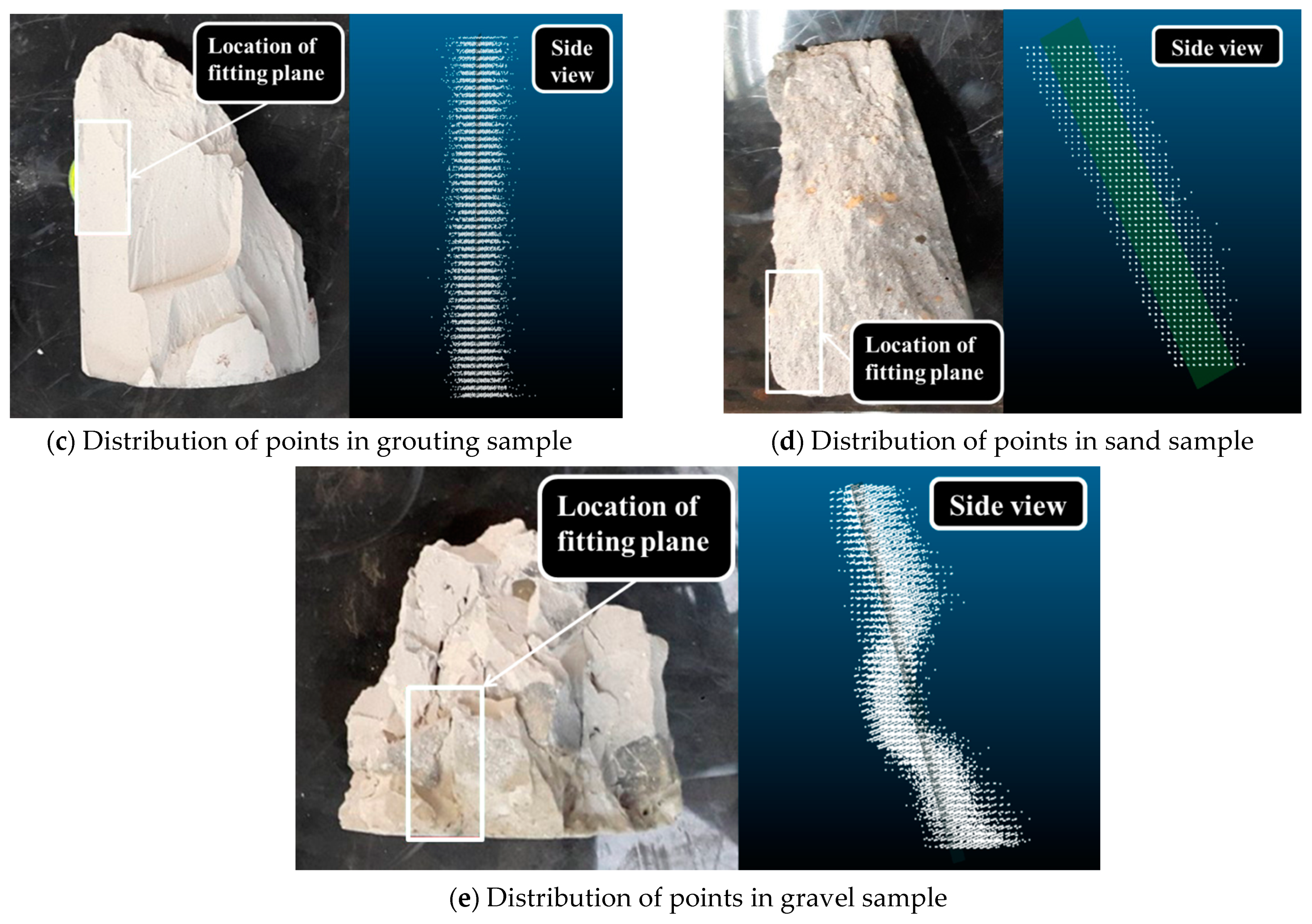
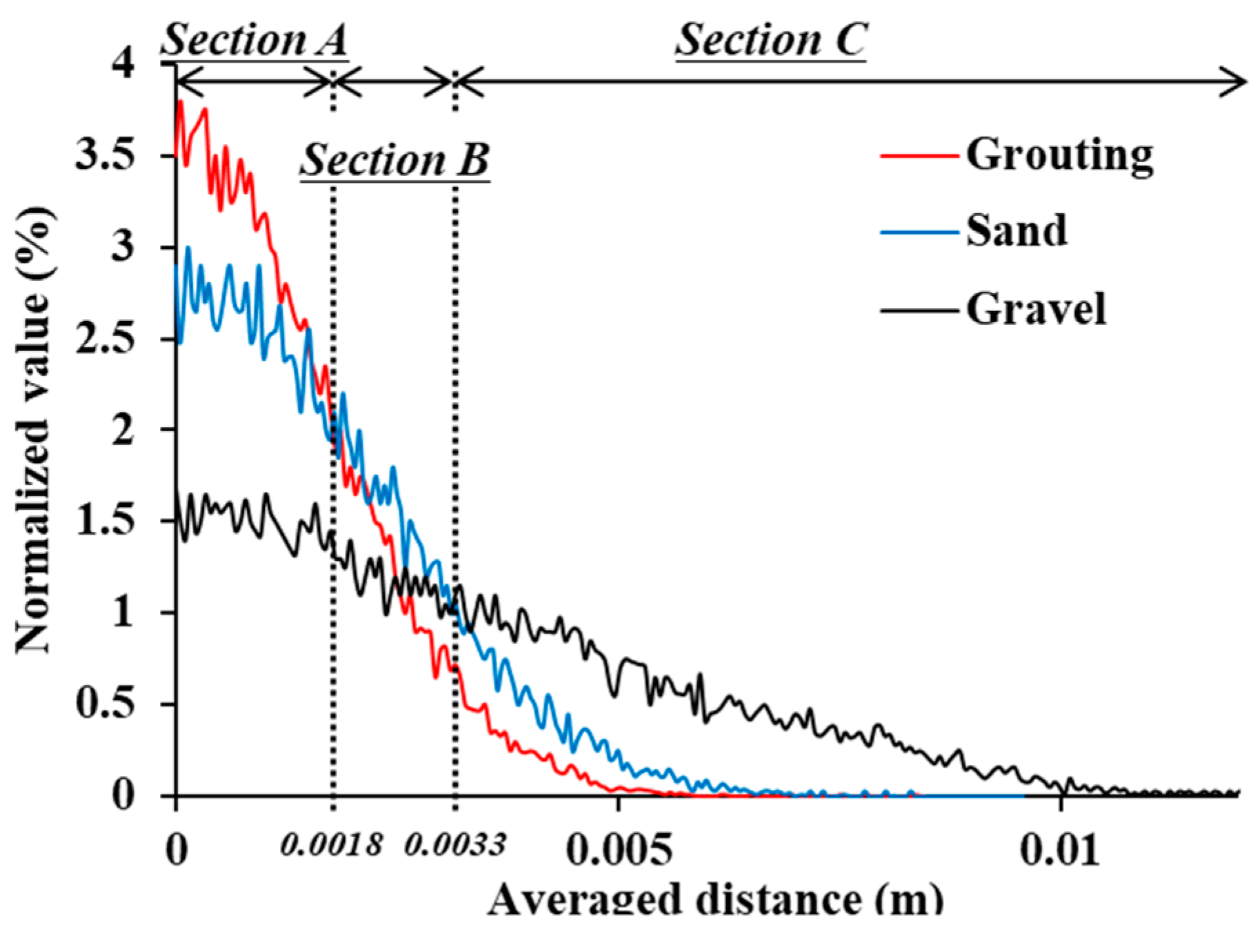
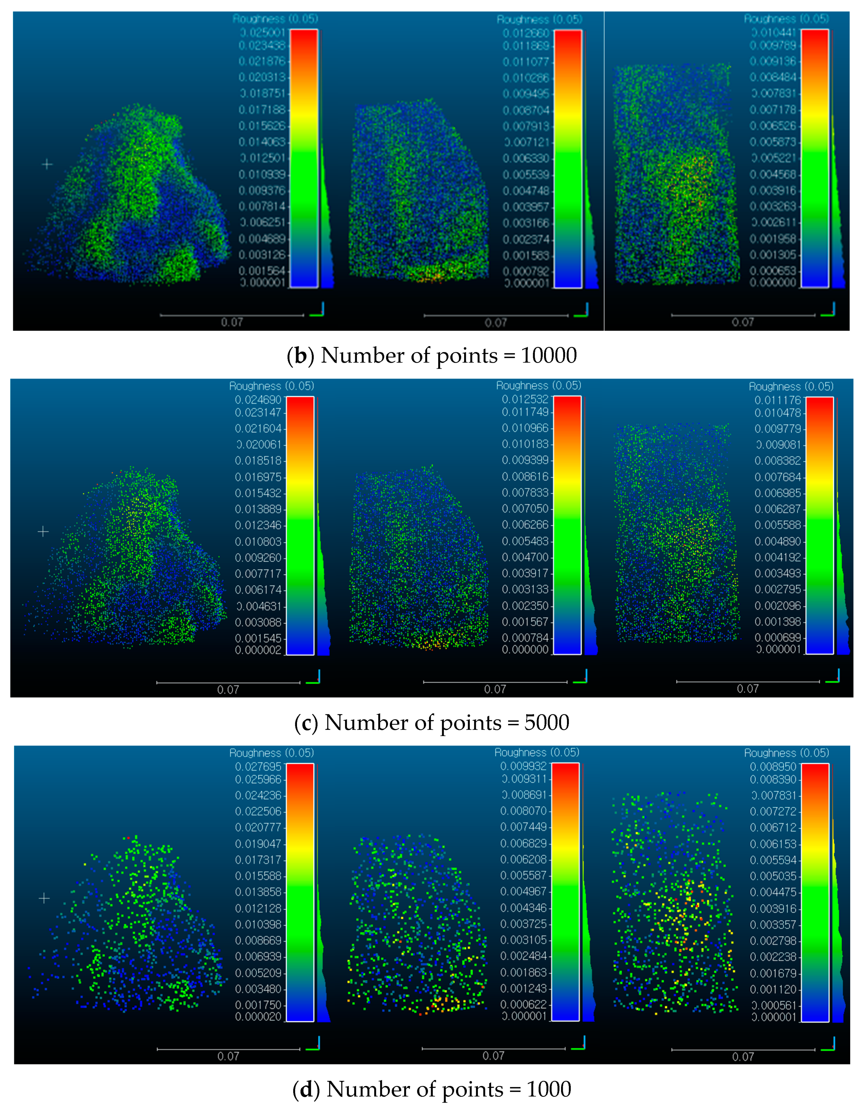
4.2. Analysis Results

A software, Cloud compare, was used to perform the analysis of the point cloud (CLOUDCOMPARE, 2018 [3]). Since the front view of the failure surface of the point cloud is a rectangle with a vertical to horizontal ratio of about 10:4 on average, the fitting surface is simulated as a rectangle. Compared to the other two samples, the roughness of the gravel has to include both the local roughness and the curvature of the gravel so that the calculation of the fitting surface can affect the result. Therefore, as shown in Figure 7a, the analysis results were compared when the sizes of the fitting plane are 25 mm × 10 mm, 50 mm × 20 mm, and 75 mm × 30 mm. It can be seen that when the size of the fitting plane is 25 length and 10 width, the C2M distance is not changed within about 2 mm. If the fitting surface is small, the curvature of some part of the gravel can be simulated, but local roughness is not appropriately simulated. When the rectangular fitting face is 75 mm long and 30 mm wide, it shows that the local roughness and curvature of the gravel are expressed in the histogram within 10 mm. However, since the fitting surface is too large for the sample size, the convex protruding shape irrespective of the roughness of the failure surface affects the result. Therefore, it can be seen that the roughness is calculated even after the C2M distance is 10 mm. When the size of the fitting surface is 50 mm in length and 20 mm in width, it is not only reflected appropriately in the C2M analysis results of local roughness and gravel curvature, but it is also possible to collect a number of analysis samples from the failure surface. As shown in Figure 7b, the point clouds of the failure surface were cut into five rectangular shapes in each sample, and the cut surfaces were overlapped with each other in the cases of gravel and grouting samples due to small size of the failure surface. Fitting planes were created from the cut point clouds, and C2M distance can be calculated. Figure 7c shows the location of the fitting plane on the failure surface of the grouting sample and the distribution of points within the fitting plane. In the side view of the distribution of the points within the fitting plane, a uniform distribution pattern is shown without large curvature in the grouting sample. An example of a fitting plane at the failure surface of a sand sample and the distribution of points within the fitting plane are shown in Figure 7d. The points are distributed in a wavy shape relative to the fitting plane by the sand grains and the local curvature on the failure surface (see side view in Figure 7d). In the gravel sample, the sharp curves of the failure surface caused by the protrusion of the gravel and the area from which the gravel is separated from the failure surface are expressed as a distribution of points. Since the fitting plane is 20 mm wide and 50 mm long, the roughness due to gravel is also revealed in the side view. The global distribution of points is not only spread over the fitting surface, but also the points are distributed farther from the fitting plane in the local area than the other samples (see Figure 7e).

Figure 8 shows the histogram of the C2M distance for each sample. Figure 8a shows the histogram of the grouting sample. The averaged C2M distance at which the number reached 95% of total points on the five histograms is 3.50 mm. Most points are concentrated within a small C2M distance range of the histogram, which means that the failure surface has a small roughness as discussed in Figure 6d. The averaged C2M distance at which the number of points in the sand sample reached 95% is 3.77 mm, which is slightly larger than that of the grouting sample (see Figure 8b). The C2M distance is increased by the roughness of the sand grain and the local roughness. As shown in Figure 8c, although the results of gravel sample are randomly different depending on the cutting position, results of five point clouds are distributed on a wider C2M distance range than the other samples, which means that the failure surface is the roughest. The averaged C2M distance of five histograms at which the number reached 95% is 5.49 mm.

4.3. Discussion

The calculated five histograms were averaged in each sample. However, the number of points is not the same among the averaged histograms of each sample, and the class interval of C2M distance of each histogram is also different. The histogram areas calculated by summation of the C2M distance class multiplied by the points are different among the different samples and hence it is not possible to compare the histograms of the three samples directly. In this paper, each histogram was normalized by the summation of the number of points at each C2M distance multiplied by each C2M distance class, which means the area of the histogram. Normalized histograms can be compared with each other because they have the same area (see Figure 9). In the grouting sample, the most points are distributed at a short C2M distance which is less than 1.8 mm (see ‘Section A’ in Figure 9). At a C2M distance of 1.8 mm, the histograms of the grouting sample and the sand sample intersected each other, and the sand sample is dominant between 1.8 and 3.3 mm. It is affected by the sand grain size of about 2 mm and local roughness (see ‘Section B’ in Figure 9). The intersection between the sand sample and the gravel sample is located at a C2M distance of 3.3 mm. The points of the gravel sample are dominantly distributed larger than 3.3 mm due to the size of gravel (see ‘Section C’ in Figure 9). In the sand and the gravel samples, the roughness or local failure of the points on the failure surface mostly occurs less than a C2M distance of 3.3 mm so that the distribution of points is reduced dramatically above a C2M distance of 3.3 mm. The proposed P2PH method can be distinguished by dividing C2M distance sections in which points of three samples are predominantly distributed. Therefore, a criterion for determining the roughness of the three-dimensional point cloud can be established by these sections.

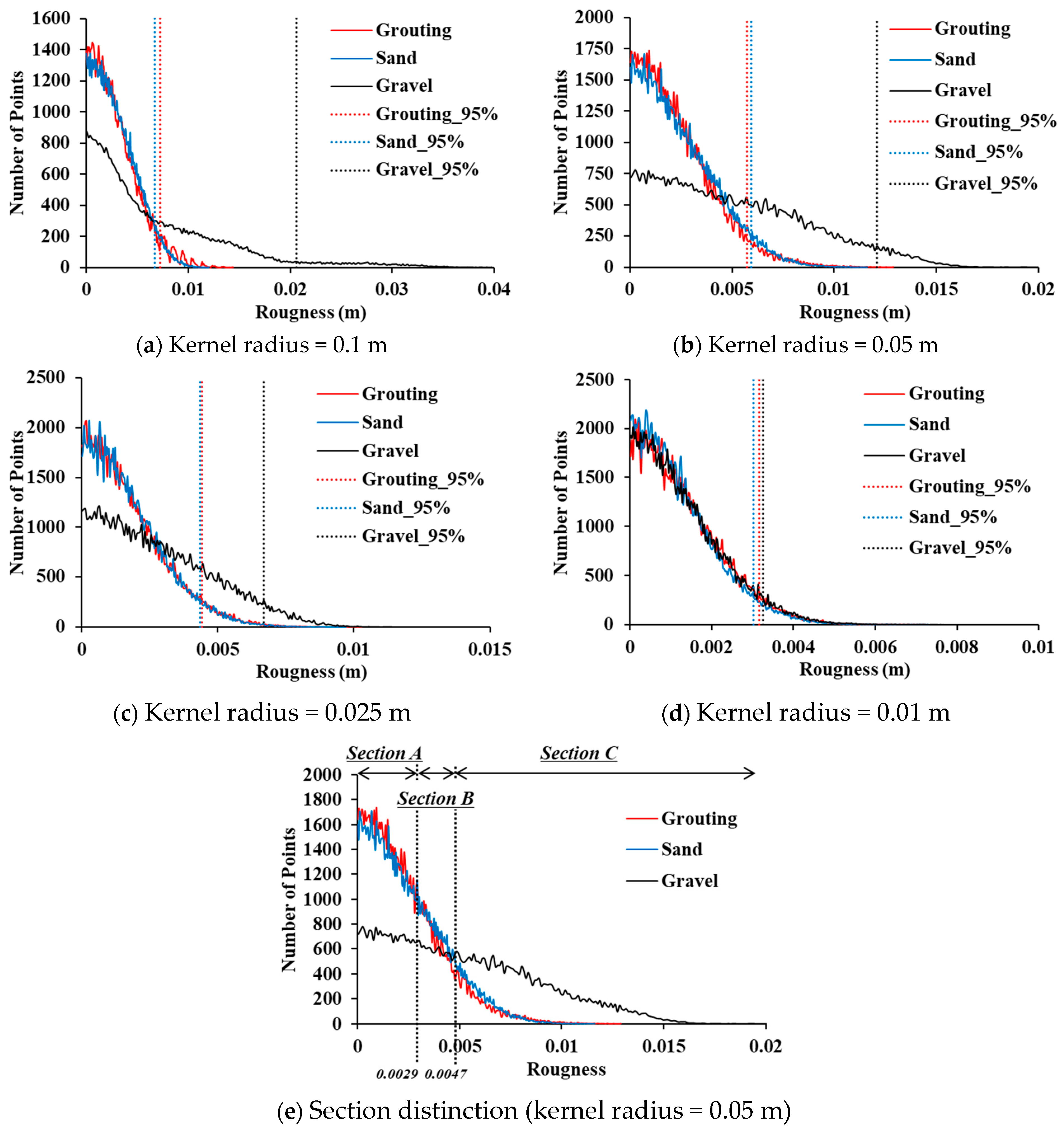
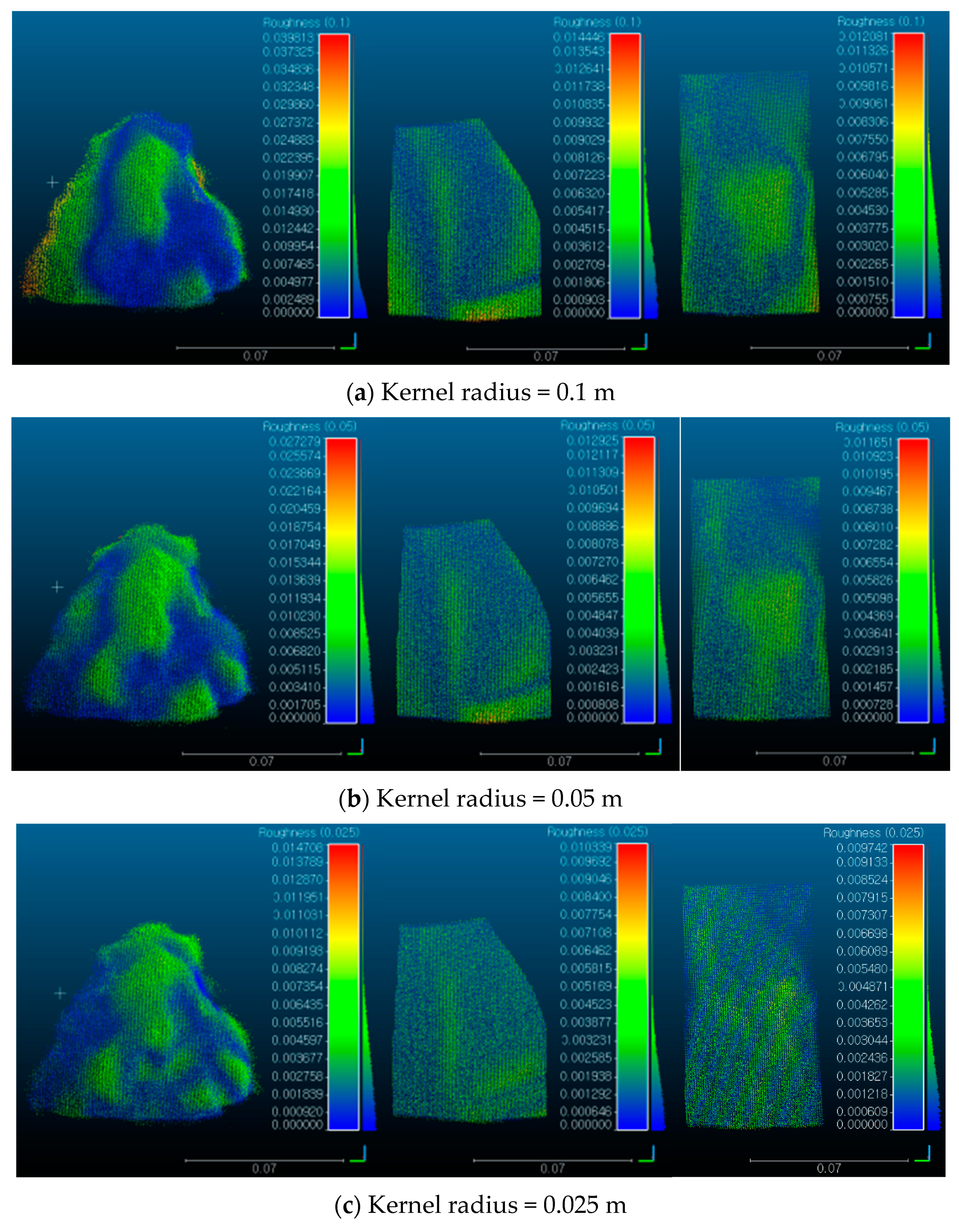
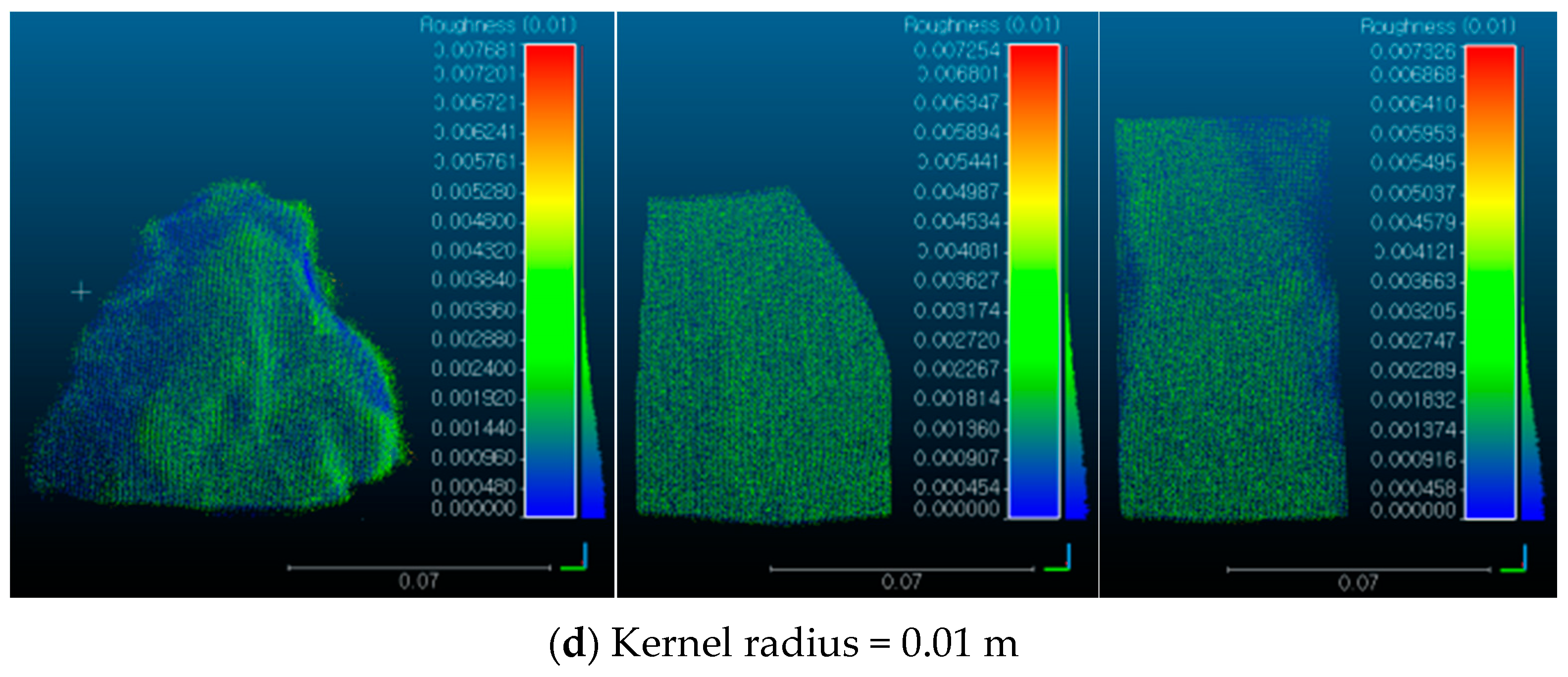
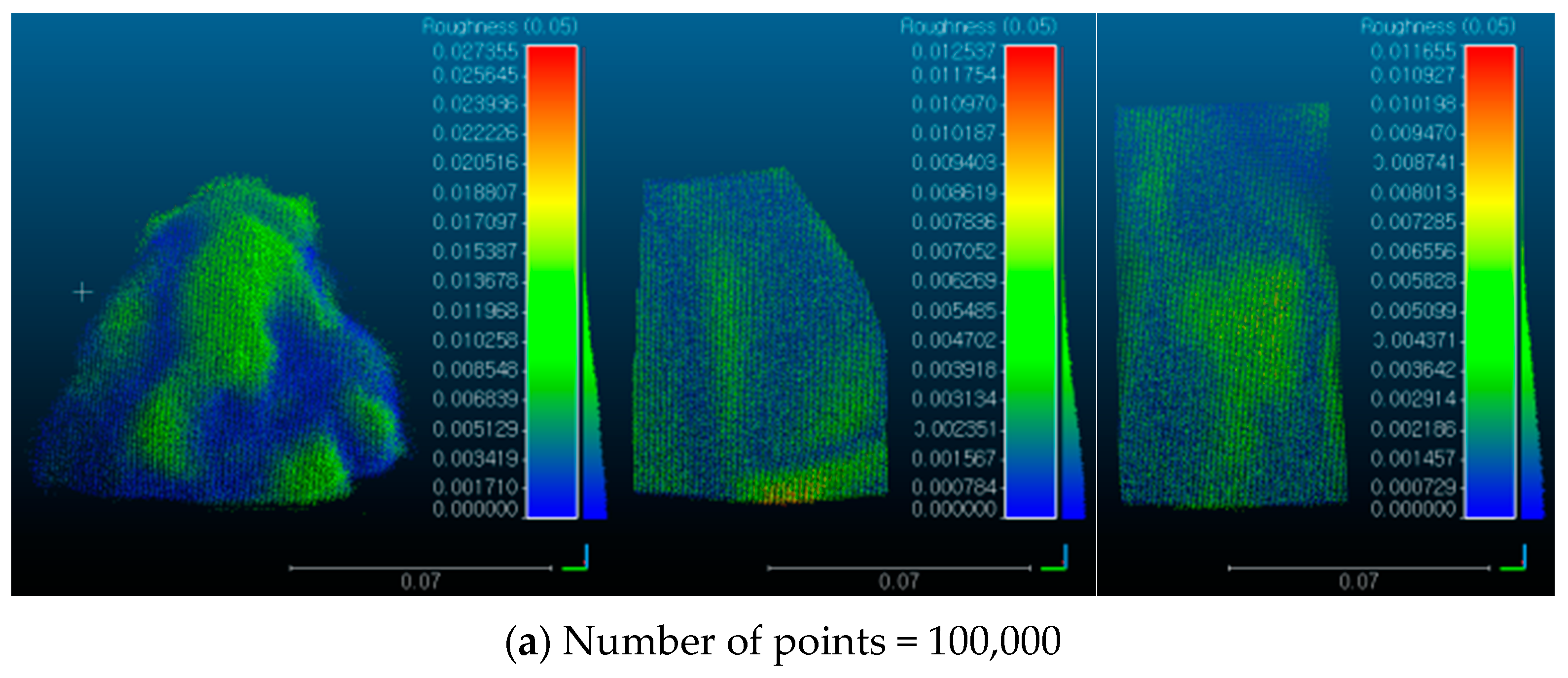
5. Analysis of Roughness Detection Method by Kernel

5.1. Analysis Method

In this paper roughness detection method by kernel was applied to estimate the three-dimensional roughness. In this method, a point cloud is projected onto the kernel and the roughness of the sample is determined by the elevation of points in the kernel. Since the three-dimensional roughness is affected by the size of the kernel measuring the roughness, the optimized kernel radius which can reflect the roughness of three samples was evaluated by the roughness analysis of changing the kernel radius. Equation (1) shows the roughness (CLOUDCOMPARE, 2018).

$$R_j=\left(\left|\mathsf{\Delta }{Z}_1|+|\mathsf{\Delta }{Z}_2|\dots |\mathsf{\Delta }{Z}_i\right|\right)/\mathrm{n}$$

(1)

where, R is roughness calculated for points within a kernel radius of j, ΔZ is the difference in elevation from a measurement point and the least squares plane calculated by the nearest neighboring measurement points, and n is the number of measurement points within a kernel radius (see Figure 10a). As shown in Figure 10b, the roughness was analyzed by changing the kernel radius to 0.01, 0.025, 0.05, and 0.1 m. The maximum kernel radius was set as 0.1 m because the diameter of the sample is 0.1 m and the longest length of the failure surface is about 0.2 m. The minimum kernel radius was set as 0.01 m considering that the diameter of the gravel is 0.02 m. When the kernel radius increases, the local roughness is diluted by other points. When the kernel radius decreases, it is difficult to reflect the global curvature of roughness. Therefore, this paper evaluated the optimized kernel radius that can best reflect the roughness of the three samples.

5.2. Analysis Results

In order to compare the three samples equivalently, the point clouds of the failure surfaces in each sample were cut to have 135,000 points each so that the histograms of each sample can be compared to each other without normalization. Figure 11a shows the results of the histogram of three samples when the kernel radius is 0.1 m. The histograms of grouting and sand samples have almost similar patterns, and the roughness at which the number of points reached 95% was 7.25 and 6.72 mm, respectively. Contrary to the results in Figure 9, the results of histograms show that the roughness of the grouting sample was slightly rougher than that of the sand sample because the kernel size is too large to reflect the local curvature of failure surface in the sand sample. In the grouting sample, the surface is generally flat, but there is a global curvature where the angle of failure surface is sharply changed at the bottom of the sample. The kernel radius of 0.1 m reflects this global roughness of the grouting sample more than the roughness caused by grains or local curvature of sand. The histogram of the gravel sample showed three inflection points, and the roughness at which the number of points reached 95% is 2.06 mm. Although the roughness caused by the gravel is reflected, the roughness is distributed over a large roughness range in the histogram because the size of the kernel is larger than the sample size. Figure 11b is the result when the kernel radius is 0.05 m, and the distribution of roughness range is narrower than the kernel radius of 0.1 m. The points of the grouting sample are slightly more than that of the sand sample within a small roughness range, and the points of sand are more increased with the increase of the roughness. Therefore, the roughness of the failure surface in the sand sample is appropriately reflected as similar as the result obtained in Figure 9. The roughness at which the number of points in the grouting sample and the sand sample reached 95% is 5.73 and 5.94 mm, respectively, showing a relevant result that the roughness of the sand sample is slightly larger. The number of points in the gravel sample linearly decreased with the increase of the roughness. The roughness at which the number of points in the gravel sample reached 95% is 1.21 mm, which is about twice as large as those of the other samples. It was found that the kernel of 0.05 m adequately reflects the roughness of the gravel because it can cover the protrusion and the traces of destruction of several gravels. Therefore, the kernel radius of 0.05 m can be a standard for calculating the three-dimensional point cloud roughness of the three samples, which can reflect the roughness features of the three samples. Figure 11c shows the histogram of three samples when the kernel radius is 0.025 m. The histograms of the grouting and sand samples show almost the same distribution, and the roughness at which the number of points in the sample reached 95% is almost the same at 4.42 and 4.36 mm, respectively. It can be seen that a kernel radius of 0.025 m is not adequate to distinguish the histograms between grouting and sand samples. However, the roughness features of the gravel sample can be appropriately distinguished with the other samples and the roughness at which the number of points reached 95% was 6.69 mm. The kernel radius of 0.01 m is indistinguishable among three histograms because the histograms of the three samples are overlapped in most of the roughness range. The roughness at which the number of points in the grouting, sand and gravel samples reached 95% is 3.16, 3.02 and 3.26 mm, respectively, showing similar values. Therefore, a kernel radius of 0.01 mm is not able to distinguish among histograms of three samples, and the roughness features of gravel cannot be reflected in the histogram. In the results of Figure 11c,d, the number of points in grouting and sand samples is distributed between about 1700 and 2100 in the roughness range of less than 0.001 m. Although the kernel radius is decreased to 0.01 m, the number of points is not increased in the roughness range of less than 0.001 m. It means that even if the kernel becomes smaller than 0.025 m, the roughness due to the grain or the local curvature of sand is not changed. Therefore, the lower bound of the kernel radius to reflect the roughness of the grouting and the sand samples is about 0.025 m. In this paper, the roughness-dominated section of the three samples was distinguished from the histogram in which the kernel radius that best reflects the roughness was selected as 0.05 m (see Figure 11e). The roughness of the grouting sample is dominant in the roughness range from 0 to 2.90 mm. The effects of local curvature of failure surface and the grain shape in the sand sample is more dominant than the other samples in the roughness range between 2.90 and 4.74 mm. If the roughness is larger than 4.74 mm, it can be seen that the roughness of the gravel sample is overwhelmingly dominant compared to the other two samples.

Figure 12 shows the color scale indicating the roughness of each point in three samples and Figure 12a shows the result of a kernel radius of 0.1 m. The kernel size is larger than the gravel sample so that the high roughness value is generated at the edges of the sample, which can be considered as an error. As shown in the results of the top of the gravel sample, the bottom of the grouting sample, and the center of the sand sample, the global curvature of the three samples is partially reflected. When the kernel radius is reduced to 0.05 m, the protrusions of the gravel sample are more clearly distinguished from the failure surface (see Figure 12b). The flat surface of the grouting sample has low roughness and the roughness at an angled section where the angle of the failure surface is sharply changed is high. The effects of grain and the local curvature change are reflected in the sand sample as well. As shown in the results of the gravel sample in Figure 12c, the roughness of the protrusion and the traces of destruction of gravels detected by a kernel radius of 0.025 m is distinguished in detail. However, the grouting sample and the sand sample show similar results because the sharp curvature of the failure surface at the bottom of the grouting sample is not reflected properly due to the small size of kernel radius and the local curvature of the sand sample is not properly reflected. When the kernel radius was reduced to 0.01 m, the roughness of all three cases is not reflected in the results and hence the roughness distribution of the three samples cannot be distinguished as with the results in Figure 11d (see Figure 12d).

The analysis of point cloud is significantly influenced by the density of the points. If each point included accurate coordinate information, accurate analysis results can be obtained with a point cloud containing many points. However, the scanning and analysis time is increased with the increase of the number of points. In this paper, a kernel size of 0.05 m, which reflects the roughness of three samples properly, was used to analyze the calculation of roughness regarding the density change of the point cloud. Subsamples with 100,000, 10,000, 5000, and 1000 points were extracted from 135,000 original point clouds to evaluate the roughness, and compared with the roughness of the original point cloud. Figure 13a shows a histogram in which roughness was determined by subsamples with 100,000 points. There is no significant difference with the results of the original point cloud in Figure 11b.

Table 1. Comparison of roughness between original point cloud and subsampled point clouds.

No. of Points	Roughness, mm (95% of Points)			Error (%)
	Grouting	Sand	Gravel	Grouting	Sand	Gravel
135,000	5.73	5.94	12.09	-	-	-
100,000	5.75	5.94	12.02	0.4	0.0	0.6
10,000	5.76	6.06	11.88	0.5	2.0	1.8
5000	5.62	5.83	11.98	1.9	1.8	0.9
1000	5.50	5.91	12.38	4.0	0.4	2.3

shows the roughness at which the number of points reached 95% in each sample. All three samples with 100,000 points have an error of less than 0.6% compared to the results of the original sample. When the number of points is reduced to 10,000, the histogram is similar to the original point cloud (see Figure 13b). In the grouting, sand and gravel samples, the roughness at which the number of points reached 95% was 5.76, 6.05, and 1.19 mm. The roughness of the sand and gravel samples showed an error of about 2% compared to the results of the original point cloud. The fluctuation between the roughness classes in the histogram becomes larger if the number of points is decreased to 5000 (see Figure 13c). Therefore, the distribution of points in individual roughness classes of the histogram is unstable. The roughness at which the number of points in each sample reached 95% has an error of about 2% compared to the result of the original point cloud. In the results of 1000 points, the fluctuation of histogram is larger than the others and the slope of the histogram is steeper within a roughness class of 5 mm (see Figure 13d). The roughness at which the number of points in the gravel sample reached 95% is increased to about 4% compared to the result of the original point cloud. The histograms of grouting and sand samples cannot be distinguished as well.

Figure 14 shows the result of the point cloud roughness in color scale for each point. In the case of 100,000 points, it is similar to the color scale result of the original point cloud, as shown in Figure 14a. If the number of points is reduced to 10,000, the locations with high roughness are still same as the results of the original point clouds (see Figure 14b). When the number of points is decreased to 5000, the distribution of points becomes sparser. In the failure surface, the intensity of the color scale representing the roughness of the protrusion of the gravel in the gravel sample, and the angled failure surface in the grouting sample is decreased with the decrease of points (see Figure 14c). The roughness is reduced compared to the result of the original point cloud because the kernel is redefined by the reduced points. Figure 14d shows the results of 1000 points, and the color scale of roughness is further reduced. The location of the kernel for detecting the roughness is changed by the sparse point cloud. The elevation between the kernel and points is more reduced by the changed kernel. Therefore, the roughness scale is decreased with the decrease of the points, which means that the roughness cannot be expressed in detail under low density conditions.

5.3. Discussion

In this paper, 10 subsamples each having 100,000, 50,000, 30,000, 10,000, 7500, 5000, 2500, and 1000 were randomly extracted from the original point clouds of three samples to identify the density effect in more detail. The distance between the randomly extracted 10 subsampled point clouds was calculated by the Cloud to Cloud (C2C) distance estimation method. The C2C distance is sensitive to the roughness of the point cloud because it directly compares the distance between a point and a point. When flat point clouds with low roughness are compared with each other, the density of the point cloud is an influencing factor to affect the distance estimation (Seo, 2021 [14]). However, when calculating the distance between two rough point clouds, the C2C distance is not only affected by the density but also the roughness. A sparse point cloud is obtained on a rough surface under the same resolution conditions. Therefore, the distance between subsamples of a rough surface is estimated to be larger than the distance between subsamples of a flat surface (see Figure 15a). In order to identify the effect of the roughness of grouting, sand, and gravel samples on the C2C distance, the C2C distance between the subsamples was calculated in conjunction with the density of the point cloud. As shown in Figure 15b, the C2C distance is decreased with the decrease of point density in all three cases. The subsampled point clouds having 100,000 points had a C2C distance of about 0.3–0.4 mm, and all three samples obtained almost the same results. However, the C2C distance increased rapidly with the decrease of the number of points, resulting in a C2C distance exceeding 2 mm in the 1000 point result (see Figure 15b).

Table 2. Averaged C2C distances of subsamples in different density.

No. of Points	Averaged C2C Distance (mm)
	Grouting	Sand	Gravel
100,000	0.03	0.03	0.04
50,000	0.17	0.19	0.22
30,000	0.35	0.37	0.41
10,000	0.78	0.80	0.85
7500	0.89	0.92	0.98
5000	1.05	1.08	1.16
2500	1.37	1.40	1.53
1000	1.89	1.94	2.12

shows that the difference of the average C2C distance among the three samples is increased with the decrease of the density. As the density of the point cloud decreases, the distance between the points of the gravel subsamples becomes farther than that of the other samples. Although more points are required to show the proper roughness in the gravel sample than the other samples, the roughness is inevitably underestimated under low density conditions. Therefore, the point cloud density of each sample required for proper roughness estimation analysis can be calculated as following the C2C distance presented in Table 2.

In this paper, P2PH and kernel methods were proposed to determine the three-dimensional roughness of the failure surface of pile samples mixed with the sand and the gravel. The failure surfaces of grouting, sand, and gravel samples were distinguished by the proposed methods, and it is expected to contribute to this study to determine not only one-dimensional or two-dimensional roughness but also three-dimensional roughness of failure surface.

6. Conclusions

(1) Plane to points histogram (P2PH) method was proposed to evaluate the three-dimensional roughness of the failure surface. The point clouds of the failure surfaces were cut by a rectangle of 20 and 50 mm to create a fitting surface representing the cut area. The histogram of the C2M distance calculated between the fitting surface and the point is a criterion for the evaluation of the roughness. For grouting, sand and gravel samples, the roughness at which the point in the histogram reached 95% is 3.50, 3.77 and 5.49 mm, respectively. Points are distributed in a narrow C2M distance range on the flat failure surface, and the points are distributed in a wide C2M distance region on the rough failure surface. In the histogram, the points are predominantly distributed below 1.8 mm for grouting samples, 1.8–3.3 mm for sand samples, and over 3.3 mm for gravel samples. It can show that the roughness of each sample is properly reflected in the histogram, and the proposed method can be a criterion for evaluating the roughness of each pile sample.

(2) A roughness detection method by the kernel was applied in this study and the elevation of points can be calculated by projecting the point cloud onto the kernel was applied. Since the roughness is affected by the kernel size significantly, the optimized kernel radius reflecting the roughness of the three samples was calculated as 0.05 m. If the kernel radius is increased, the local roughness is diluted by other points and the roughness decreases. If the kernel radius is decreased, it is not able to reflect the global curvature of the failure surface.

(3) The roughness detection method by the kernel is affected by the density of the point cloud, and hence the roughness analysis to define the effect of the point cloud density was performed. It is proposed that more than 5000 points need to be obtained within the cut point cloud to clearly distinguish the roughness.

(4) In order to define the density effect, subsamples were extracted from the original point clouds of three pile samples and then the C2C distance between subsamples was calculated. The C2C distance and the C2C distance difference between samples are also rapidly increased with the decrease of density. If the failure surface is rougher such as gravel, it is more affected by density reduction than the other samples.

The research on 3D roughness analysis performed in this paper is expected to be conducive to studies that require roughness estimation in the future. Since roughness is an important factor in shear behavior, studies using three-dimensional roughness to calculate shear strength can be conducted as a prospective study.

References

1. Battista, N.D.; Kechavarzi, C.; Seo, H.; Soga, K.; Pennington, S. Distributed Fibre Optic Sensors for Measuring Strain and Temperature of Cast-in-situ Concrete Test Piles. In Proceedings of the International Conference on Smart Infrastructure and Construction Construction, Cambridge, UK, 27–29 June 2016. [Google Scholar]
2. Bauret, S.; Rivard, P. Experimental Assessment of the Tensile Bond Strength of Mortar-Mortar Interfaces: Effects of Interface Roughness and Mortar Strength. Geotech. Test. J. 2018, 41, 1139–1146. [Google Scholar] [CrossRef]
3. CLOUDCOMPARE. CloudCompare 2.9.1 ed. 2018. Available online: https://www.danielgm.net/cc/ (accessed on 17 March 2021).
4. Farrell, E.R.; Lawler, M.L. CFA pile behaviour in very stiff lodgement till. Proc. Inst. Civ. Eng. Geotech. Eng. 2008, 161, 49–57. [Google Scholar] [CrossRef]
5. Gavin, K.G.; Cadogan, D.; Casey, P. Shaft Capacity of Continuous Flight Auger Piles in Sand. J. Geotech. Geoenviron. Eng. 2009, 135, 790–798. [Google Scholar] [CrossRef]
6. Hong, E.-S.; Lee, I.-M.; Lee, J.-S. Measurement of Rock Joint Roughness by 3D Scanner. Geotech. Test. J. 2006, 29, 482–489. [Google Scholar]
7. Lee, D.-H.; Juang, C. A New Technique for Measuring the Roughness Profile of Rock Joints. Geotech. Test. J. 1991, 14, 320. [Google Scholar]
8. Leznicki, J.K.; Esrig, M.I.; Gaibrois, R.G. Loss of Ground during CFA Pile Installation in Inner Urban Areas. J. Geotech. Eng. 1992, 118, 947–950. [Google Scholar] [CrossRef]
9. Li, Y.; Mo, P.; Aydin, A.; Zhang, X. Spiral Sampling Method for Quantitative Estimates of Joint Roughness Coefficient of Rock Fractures. Geotech. Test. J. 2018, 42, 245–255. [Google Scholar] [CrossRef]
10. Loveridge, F.; Cecinato, F. Thermal performance of thermoactive continuous flight auger piles. Environ. Geotech. 2016, 3, 265–279. [Google Scholar] [CrossRef]
11. Pelecanos, L.; Soga, K.; Elshafie, M.Z.E.B.; Battista, N.; Kechavarzi, C.; Gue, C.Y.; Ouyang, Y.; Seo, H.J. Distributed Fibre Optic Sensing of Axially Loaded Bored Piles. J. Geotech. Geoenviron. Eng. 2018, 144, 1–16. [Google Scholar] [CrossRef] [Green Version]
12. Rauthause, M.P.; Stuedlein, A.W.; Olsen, M.J. Quantification of Surface Roughness Using Laser Scanning with Application to the Frictional Resistance of Sand-Timber Pile Interfaces. Geotech. Test. J. 2020, 43, 966–984. [Google Scholar] [CrossRef]
13. Seo, H. Monitoring of CFA pile test using three dimensional laser scanning and distributed fiber optic sensors. Opt. Lasers Eng. 2020, 130, 106089. [Google Scholar] [CrossRef]
14. Seo, H. Long-term Monitoring of zigzag-shaped concrete panel in retaining structure using laser scanning and analysis of influencing factors. Opt. Lasers Eng. 2021, 139, 106498. [Google Scholar] [CrossRef]
15. Seo, H.J.; Jeong, K.H.; Choi, H.S.; Lee, I.M. Pullout Resistance Increase of Soil Nailing Induced by Pressurized Grouting. J. Geotech. Geoenviron. Eng. 2012, 138, 604–613. [Google Scholar] [CrossRef]
16. Seo, H.J.; Lee, I.M.; Lee, S.W. Optimization of Soil Nailing Design Considering Three Failure Modes. KSCE J. Civil Eng. 2014, 18, 488–496. [Google Scholar] [CrossRef]
17. Seo, H.J.; Lee, I.M.; Ryu, Y.M.; Jung, J.H. Mechanical Behavior of Hybrid Soil Nail-Anchor System. KSCE J. Civil Eng. 2019, 23, 4201–4211. [Google Scholar] [CrossRef]
18. Seo, H.J.; Pelecanos, L.; Kwon, Y.S.; Lee, I.M. Net Load-displacement Estimation in Soil-nailing Pullout Tests. Proc. Inst. Civil Eng. Geotech. Eng. 2017, 170, 534–547. [Google Scholar] [CrossRef] [Green Version]
19. Seo, H.; Zhao, Y.; Wang, J. Monitoring of Retaining Structures on an Open Excavation Site with 3D Laser Scanning. In Proceedings of the International Conference on Smart Infrastructure and Construction 2019 (ICSIC), Cambridge, UK, 8–10 July 2019; ICE Publishing: London, UK, 2019; pp. 665–672. [Google Scholar]
20. Sethy, B.P.; Patra, C.R.; Das, B.M.; Sobhan, K. Bearing Capacity of Circular Foundation on Sand Layer of Limited Thickness Underlain by Rigid Rough Base Subjected to Eccentrically Inclined Load. Geotech. Test. J. 2018, 42, 597–609. [Google Scholar] [CrossRef]
21. Sobola, D.; Talu, S.; Sadovsky, P.; Papez, N.; Grmela, L. Application of AFM Measurement and Fractal Analysis to Study the Surface of Natural Optical Structures. Adv. Electr. Electron. Eng. 2017, 15, 569—576. [Google Scholar] [CrossRef]
22. Soga, K.; Kwan, V.; Pelecanos, L.; Rui, Y.; Schwamb, T.; Seo, H.; Wilcock, M. The Role of Distributed Sensing in Understanding the Engineering Performance of Geotechnical Structures. In Proceedings of the 15th European Conference on Soil Mechanics and Geotechnical Engineering, Edinburgh, UK, 13–17 September 2015. [Google Scholar]
23. Tehrani, F.S.; Han, F.; Salgado, R.; Prezzi, M.; Tovar, R.D.; Castro, A.G. Effect of surface roughness on the shaft resistance of non-displacement piles embedded in sand. Géotechnique 2016, 66, 386–400. [Google Scholar] [CrossRef]
24. Tran, T.V.; Tucker-Kulesza, S.E.; Bernhardt-Barry, M.L. Determining Surface Roughness in Erosion Testing Using Digital Photogrammetry. Geotech. Test. J. 2017, 40, 20160277. [Google Scholar] [CrossRef]
25. Wang, Z.; Gu, L.; Shen, M.; Zhang, F.; Zhang, G.; Deng, S. Influence of Shear Rate on the Shear Strength of Discontinuities with Different Joint Roughness Coefficients. Geotech. Test. J. 2019, 43, 683–700. [Google Scholar] [CrossRef]
Figure 1. Soil collapsing effect in CFA pile.
Applsci 11 02713 g001
Figure 2. Test samples for surface roughness analysis.
Applsci 11 02713 g002
Figure 3. Scanning of three samples.
Applsci 11 02713 g003
Figure 4. Schematic diagram of point cloud in three samples.
Applsci 11 02713 g004aApplsci 11 02713 g004b
Figure 5. Three-dimensional point clouds of pile samples.
Applsci 11 02713 g005
Figure 6. Cloud compare analysis using fitting plane.
Applsci 11 02713 g006
Figure 7. Fitting planes and distribution of points within the fitting plane for each sample.
Applsci 11 02713 g007aApplsci 11 02713 g007b
Figure 8. Distance distribution between the fitting plane and point clouds.
Applsci 11 02713 g008
Figure 9. Normalized histogram for three samples.
Applsci 11 02713 g009
Figure 10. Estimation of roughness kernel.
Applsci 11 02713 g010
Figure 11. Roughness histograms for of three samples with different kernel radius.
Applsci 11 02713 g011
Figure 12. Color scale indicating the degree of roughness of the cloud.
Applsci 11 02713 g012aApplsci 11 02713 g012b
Figure 13. Effect of point cloud density on roughness.
Applsci 11 02713 g013aApplsci 11 02713 g013b
Figure 14. Color scale of roughness with different density of point cloud.
Applsci 11 02713 g014aApplsci 11 02713 g014b
Figure 15. C2C results between subsamples with different density.
Applsci 11 02713 g015