Monitoring Scheme for the Detection of Hydrogen Leakage from a Deep Underground Storage. Part 2: Physico-Chemical Impacts of Hydrogen Injection into a Shallow Chalky Aquifer

Featured Application

Implementation of a physicochemical and hydrogeochemical monitoring in shallow aquifers above future underground hydrogen storage sites in salt caverns.

Abstract

This paper presents the results of an experiment to simulate a sudden and brief hydrogen leak from a potential deep geological storage site. A 5 m³ volume of groundwater was extracted, saturated with hydrogen, and then reinjected into the aquifer. Saturating the water with hydrogen caused a decrease in the oxidation-reduction potential, the dissolved gas content (especially O₂ and CO₂), the electrical conductivity, and the concentration of alkaline earth bicarbonate ions and a slight increase in pH. These changes are observed until 20 m downstream of the injection well, while the more distant piezometers (from 30 to 60 m) are not significantly affected. During this experiment, no indicators of the development of chemical or biochemical reactions are observed, because of the rapid transfer of the dissolved hydrogen plume through the aquifer and its significant dilution beyond 10 m downstream of the injection well. Here, hydrogen behaved as a conservative element, reacting very slightly or not at all. However, this experiment demonstrates the existence of direct and indirect impacts of the presence of hydrogen in an aquifer. This experiment also highlights the need to adapt the monitoring of future underground hydrogen storage sites.

1. Introduction

1.1. General Information on Underground Hydrogen Storage

In 2015, France promulgated the Law on Energy Transition for Green Growth in order to contribute more effectively to the fight against climate change and the preservation of the environment, as well as to strengthen its energy independence [1]. This law aims in particular to develop renewable energy sources, some of which are of a fluctuating or intermittent nature and thereby require significant storage capacity. The underground environment is well suited to large-scale storage, and France already has 78 salt caverns with a capacity to store liquid or liquefied hydrocarbons as well as natural gas [2]. The gradual phasing out of fossil fuels gives rise to the hypothesis that future underground storages of hydrogen (H₂) will need to be developed, as already in the United Kingdom or the United States [3]. This technology is likely to be of interest to several European countries: Germany, the Netherlands, Denmark, Poland, France, etc. [4].

This is why the French Scientific Interest Group GEODENERGIES chose to fund a research project in 2017 on the risks and opportunities of the geological storage of hydrogen in salt caverns, entitled ROSTOCK-H. Among other things, this project focuses on the risks associated with possible hydrogen gas leaks from deep storage. In the event of such leakage, the hydrogen would migrate to the surface and encounter at least one aquifer where the gas would dissolve in the water until saturation [5]. However, considering the very low solubility of this gas (in the order of 1.8 mg·L⁻¹ at saturation under surface conditions), there is a risk that the leak flow rate may exceed the dissolution potential for hydrogen in water. In this case, part of the gas would continue its migration to the surface in gaseous form until it encounters an impermeable formation or a void where it can accumulate (mine, underground networks, cellar, underground car park, tunnel, etc.): hydrogen may then cause asphyxiation or, due to its very weak lower flammability limit (around 4%), explosion or fire [2].

To study the risks associated with this new storage technology, particularly in the event of a leak towards the surface, we carried out an experiment to simulate a hydrogen leakage from a possible deep geological storage. To do this, we injected hydrogen into the chalk aquifer, which is a major drinking water resource in the Paris region. Several monitoring devices were set up directly in the aquifer up to 60 m downstream from the injection point, in order to monitor the evolution of the dissolved hydrogen plume and the associated physico-chemical and hydrochemical phenomena. Under the proposed experimental conditions, and due to the brevity of the injection, we did not expect any biochemical reactions that require long time scales to occur. Moreover, additional studies [6,7,8,9] pointed out that a sudden injection of hydrogen saturated water into an aquifer increases the dissolved hydrogen content of the water, and consequently reduces its oxidation-reduction potential, as well as the concentration of other dissolved gases (O₂, CO₂, N₂, etc.). The injection of hydrogen was preceded by the injection of tracers (helium and hydrogeological tracers) in order to facilitate the monitoring of its progress underground. This experiment was conducted at the Catenoy (Oise) experimental site in a surface aquifer representative of the carbonated hydrogeological context of the Paris Basin. It followed characterization work for this site, previously carried out during CO₂ leak simulations [10,11], as well as the realization of a baseline and a preliminary injection of helium [6].

1.2. Hydrogen Reactivity in a Natural Environment

The impacts expected from a hydrogen leak in the underground environment are linked to the fact that it is a strongly reducing gas acting as a potential electron donor for numerous chemical species: metal sulfides, sulfates, carbonates, oxides (in particular of iron and magnesium), nitrates, ferrous ions, and gases (CO and CO₂) [7,8]. The resulting oxidation-reduction reactions can thus modify the chemical composition of water or the mineral composition of aquifer rocks [6]. However, most reactions that occur in the presence of hydrogen require—at least in the laboratory—high temperatures or pressures or the presence of catalysts (

Table 1. Some examples of abiotic reductions due to H₂ under experimental laboratory conditions.

Impacted Species	H2 Partial Pressure (bar)	Temperature (°C)	pH	Catalyst	Resulting Species	Reference
SO42−	4–16	250–300	≤5.6	None	H2S	[13]
FeS2 *	8–18	90–180	6.9–8.7	None	FeS1+x, H2S	[14]
FeS2 *	3–30	90–250	7.8–9.8	None	FeS1+x, H2S	[12]
NO3−	0.1	22	7.0–8.7	Fe	NO2−	[15]
NO3−	0.05	200	~6	Fe	NH4+	[16]
NO3−	7.5	90–180	4–9	Carbon steel	NH4+	[17]
NO3−	0.2–7.5	90–150	4–9	Stainless steel	NH4+	[18]
NO3−	0.1–0.5	7–25	5–11	Pd, Cu	N2	[19,20]

* Pyrite transformed into pyrrhotite (FeS_1+x with 0 < x < 0.125).

). Under ambient conditions, hydrogen-consuming oxidation-reduction reactions have slow kinetics because hydrogen is not a polar molecule and the H-H bond is difficult to break owing to its elevated binding energy (436 kJ·mol⁻¹). However, Truche et al. [12] showed that the reduction of pyrite by hydrogen could have significant kinetics at low pressure and temperature in the presence of catalysts, in this case clay minerals. According to these authors, catalysts could also be bacteria, other mineral surfaces, or certain metals (iron, carbon steel, stainless steel, copper, nickel, platinum, and palladium). In the case of shallow aquifers, frequently used for water production (wells and boreholes for drinking, agricultural, industrial, or mineral water) or potentially crossed by other types of underground structures (wells, geotechnical foundations, etc.), the presence of metal parts made of iron, steel, or stainless steel could therefore play this catalytic role locally (Table 1).

In addition, the natural leak analogs, which are the hydrogen emission sites, also show that the surface and subsurface environments affected by these emissions can be significantly altered, even under ambient temperature and pressure: e.g., decrease in sulfates, decrease in oxidation-reduction potential, and increase in pH [9]. However, these are usually biogeochemical reactions that also have slow kinetics [12,21,22]. As such, the laboratory experiment carried out by Berta et al. [22] under ambient conditions lasted 180 days: it demonstrated a biochemical reduction of sulfates and carbon dioxide, a decrease in the calcium concentration, and an increase in the silica concentration concurrent with an increase in pH.

1.3. Risk of Contamination of Drinking Water Aquifers

Monitoring the aquifers would therefore be a way of detecting an ongoing hydrogen leak, for alerting purposes, especially since this gas is not generally present in groundwater. In the hydrogeological context of the Paris Basin, two aquifers could fulfill the role of barrier and surveillance zone: the deep Albian-Neocomian aquifer and the shallow Cretaceous chalk aquifer. The latter contains a generally unconfined water table which is used to supply drinking water to a part of Paris and almost all of the neighboring towns. When it is close to the surface, its water is oxygenated, thus under oxidizing conditions, and often enriched with nitrates from anthropogenic surface activities, as well as, locally, with sulfates from the overlying Tertiary formations. The arrival of hydrogen in such an aquifer has the immediate effect of increasing the dissolved hydrogen content of the water and, as a result, reducing its oxidation-reduction potential and possibly its content in natural dissolved gases (mainly N₂, O₂, and CO₂). The hydrogeochemical impacts expected in the aquifer zone affected by the presence of hydrogen could be as follows [12,13,15,16,17,22,23]:

• Reduction of nitrates (NO₃⁻) to nitrites (NO₂⁻), or even to ammonium (NH₄⁺), and then to gaseous nitrogen (N₂)
• Reduction of sulfates (SO₄²⁻) to sulfides (SO₃⁻), or even to hydrogen sulfide (H₂S)
• Reduction of iron III to iron II
• Dissolution of metallic trace elements potentially present in the aquifer rock following the drop in the redox potential

The consequences of a possible reduction in ion oxides such as NO₃⁻ can be significant because the standards for drinking water destined for human consumption stipulate 50 mg·L⁻¹ for nitrates against 0.50 mg·L⁻¹ for nitrites and 0.10 mg·L⁻¹ for ammonium [24]. Thus, allowing for a mean concentration of nitrates of 33 mg·L⁻¹ in the groundwater at the Catenoy experimental site, during the baseline [6], it would be sufficient to reduce only 2% of these ions into nitrites or 0.5% into ammonium to render the water unfit for human consumption in the first case or to trigger health warning measures (information, reinforced surveillance, treatment) in the second case.

However, the literature shows that, under normal pressure and temperature conditions, the reduction of these nitrates and sulfates cannot take place except in the presence of a catalyst such as iron, nickel, copper, or platinum. Nevertheless, the frequent use of iron and stainless steel, which contains up to 20% of nickel, in the composition of the metal tubing of underground structures will likely bring some of these catalysts into contact with the groundwater. This paper describes a specific monitoring scheme which has been applied on a pilot site allowing to follow the impacts of H₂ injection into a shallow chalky aquifer. For this, many chemical-physical parameters are monitored as well as some dissolved gases such as H₂ and O₂. The temporal evolution of all these parameters is compared in order to better understand the effect of a sudden appearance of H₂ in an aquifer and assess our ability to detect H₂ leaks.

2. Material and Methods

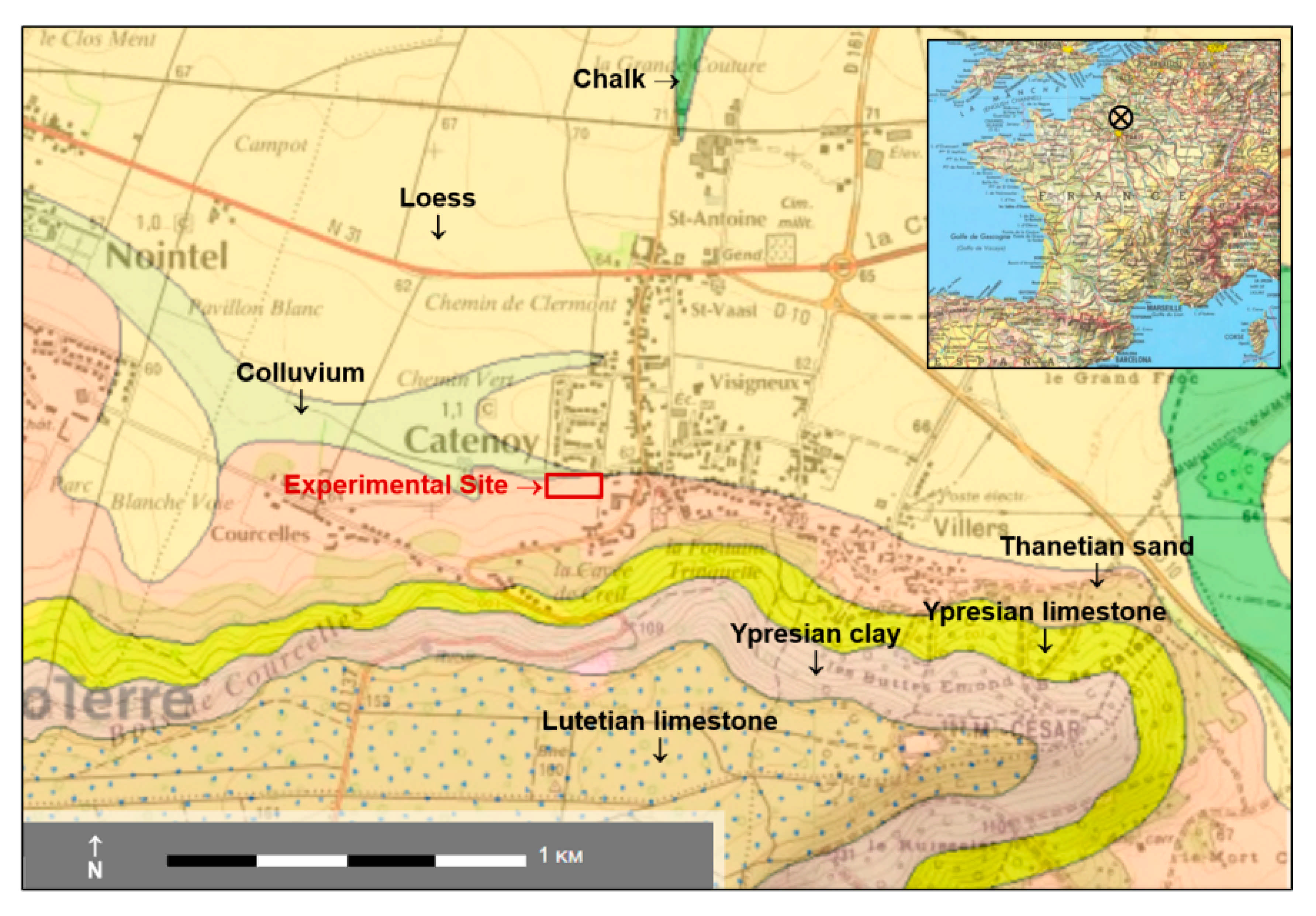
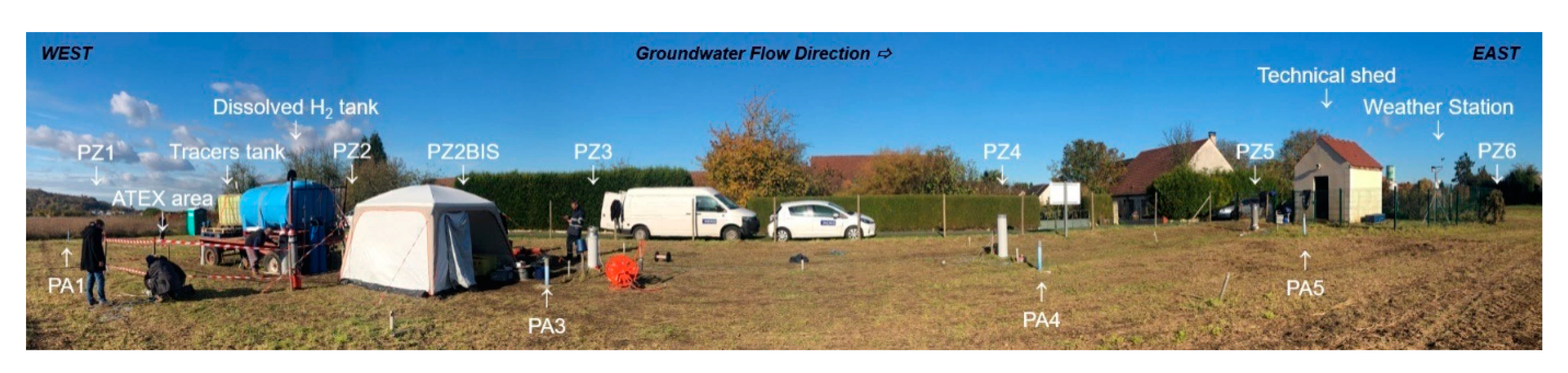
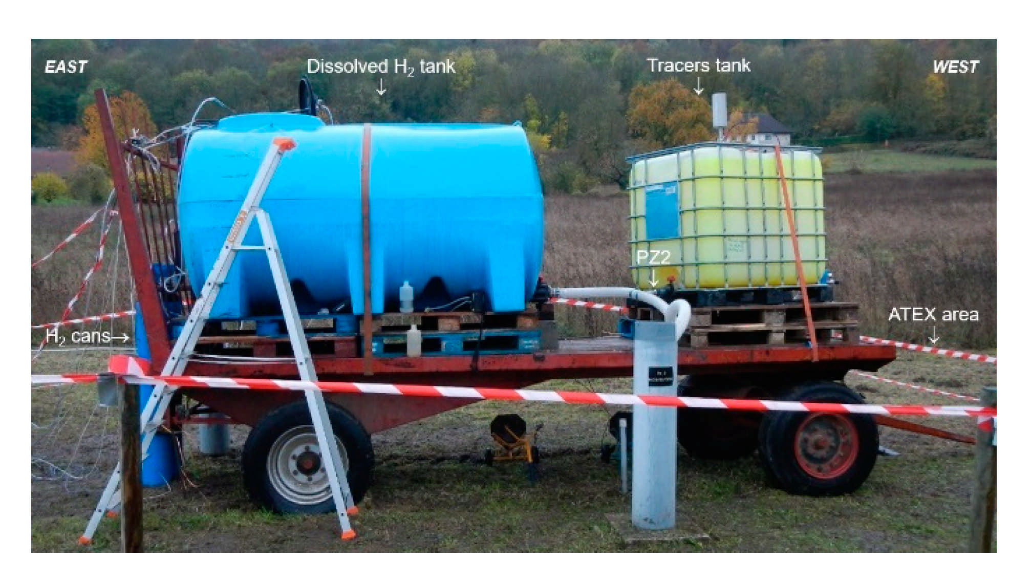
2.1. Overview of the Site Context and Equipment

The experimental site is located at Catenoy (Oise), about 50 km north of Paris [6]. It is situated in the unconfined chalk aquifer of the Paris Basin. The geology corresponds to a few meters of Quaternary deposits and Tertiary formations, lying over a hundred meters of Senonian chalk that is only visible in the thalwegs (see also Figure 1). Under the site, the underground geology of the first 25 m is: 3 m of colluvium, 4 m of Thanetian sands, and 18 m of chalk. The chalk encloses an aquifer with a static level at a depth of 13 m, which flows in the WSW–ENE direction. The storage coefficient is from 1.1 × 10⁻² to 6.5 × 10⁻² and the hydraulic conductivity is from 6.4 × 10⁻⁴ to 1.4 × 10⁻³ m·s⁻¹.

The experimental site has eight piezometers which are 25 m deep and aligned in the direction of the aquifer flow (Figure 2), over a distance of 80 m. The PZ1 piezometer, which functions as a control, is located 20 m upstream of the PZ2 injection well. The PZ3, PZ4, PZ5, and PZ6 piezometers are, respectively, located 10, 20, 30, and 60 m downstream of the injection well. There are also two close monitoring piezometers: the PZ2BIS located at 5 m, which is the main monitoring piezometer for this study, and the PZ2TER located at 7.5 m, which contains Infrared and Raman spectrometers (the specific results from these are the subject of another article in preparation). The site is also equipped with a technical room and a meteorological station. The data are transmitted in real time to the dedicated e.cenaris cloud monitoring system [25,26].

The hydrodynamic characteristics of the aquifer were determined during a pumping test carried out previously [10]. Depending on the piezometer considered, the porosity varies from 1.1 × 10⁻² to 6.5 × 10⁻² and the hydraulic conductivity from 6.4 × 10⁻⁴ to 1.4 × 10⁻³ m·s⁻¹. The groundwater flow velocity, measured during a tracing test, varies from 3 m·day⁻¹ at PZ3 and PZ5 to 10 m·day⁻¹ at PZ4, which is situated in a preferential flow path (probably a fissured zone). This highlights the dual porosity of the aquifer studied, which may be reflected hydrogeologically by contrasts in flow velocity and variations in transit times from one piezometer to another.

2.2. Overview of the Monitoring Protocol

The monitoring protocol for the saturated zone was detailed by Lafortune et al. [6] and is based on the preliminary injection of helium, because hydrogen and helium have a comparable physical behavior, in particular a very low solubility and a high diffusion coefficient in water.

As a reminder, the monitoring protocol includes (Figure 3):

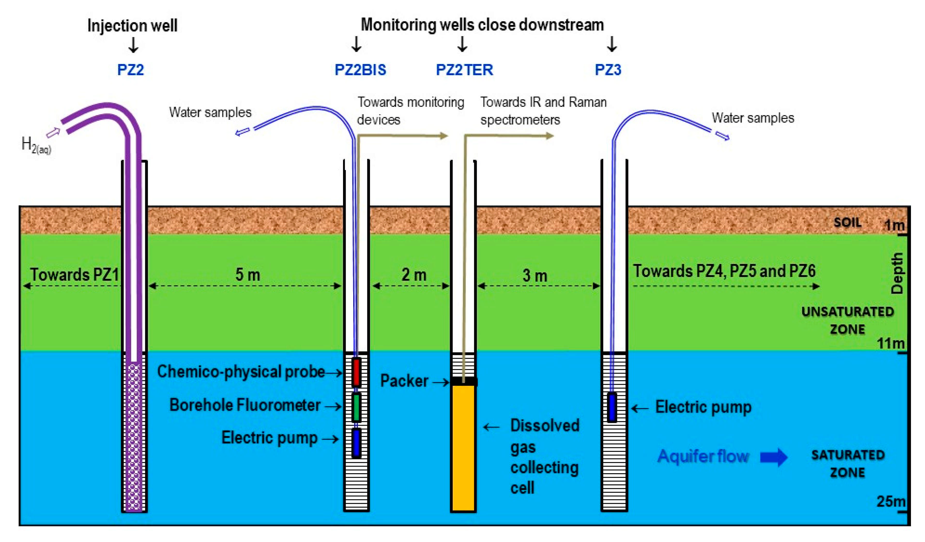
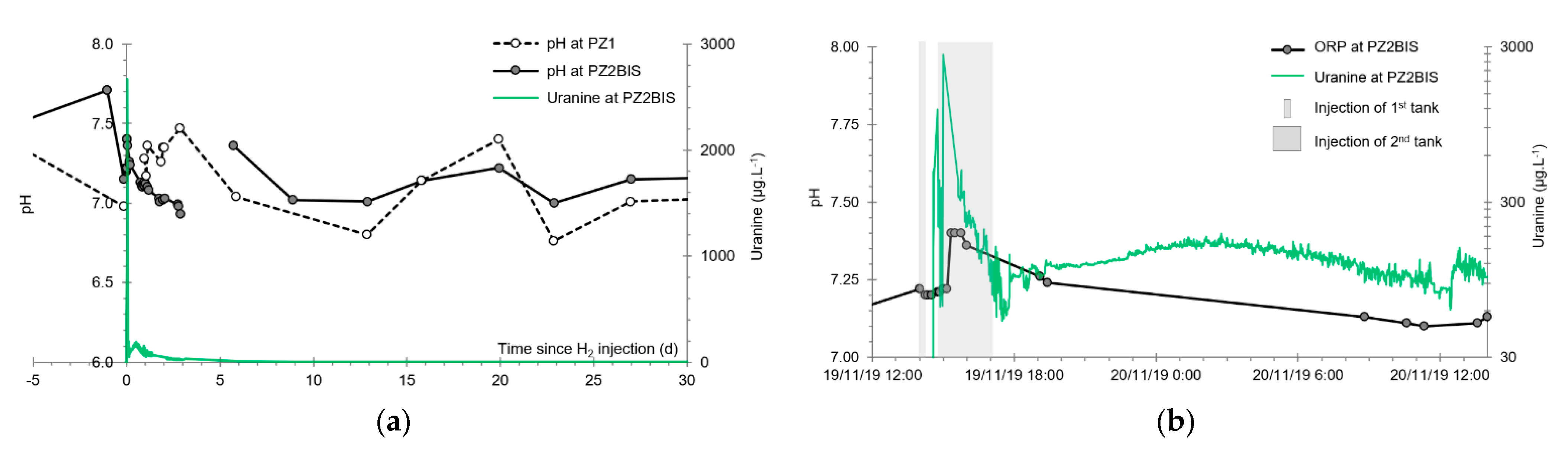
• Two physicochemical probes measure temperature, pH, electrical conductivity, oxidation-reduction potential, and dissolved oxygen. One is installed in the PZ2bis while the other is mobile in order to take measurements at all the piezometers. It should be noted that this last probe had to be replaced on 19 November 2019 at 14:00, which is visible on the graphs as a deviation due to the new calibration (just before the injection of dissolved hydrogen).
• Two field fluorometers allow on site measure of the water fluorescence. As before, one is installed in the PZ2bis, while the other is mobile in order to take measurements in all the piezometers by groundwater sampling.
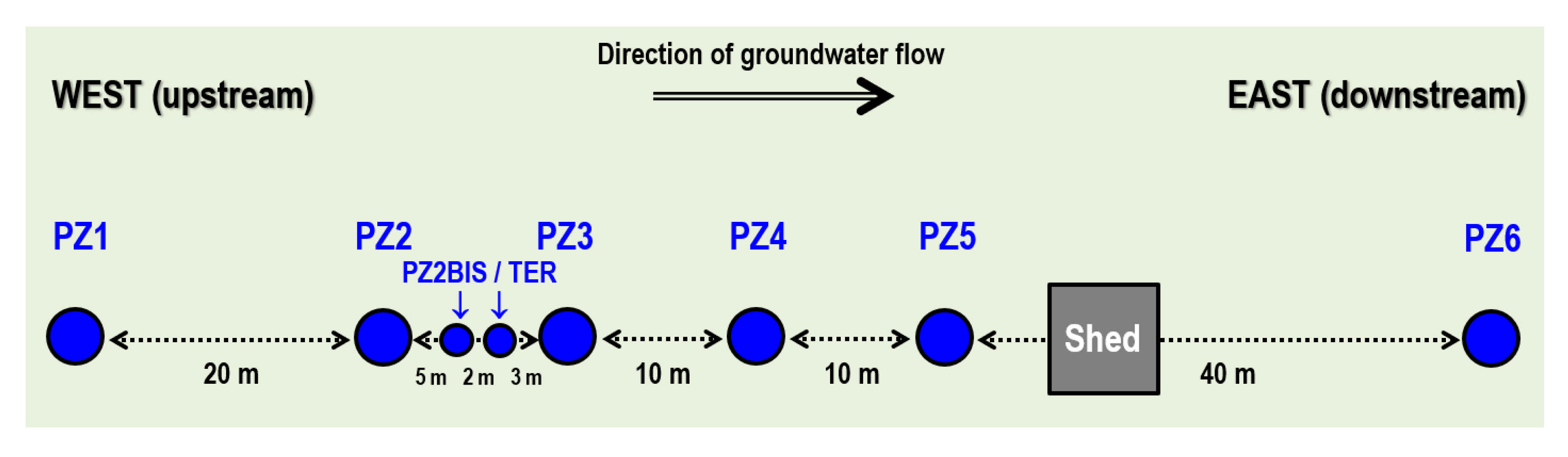
• Six submerged electric pumps are installed at a depth of 16 m at the PZ1, PZ2BIS, PZ3, PZ4, PZ5 and PZ6 piezometers. They are used to regularly sample the groundwater in order to perform laboratory analyses of tracers, dissolved gases (CH₄, He, H₂, and H₂S), major elements (Ca²⁺, Mg²⁺, Na⁺, K⁺, HCO₃⁻, Cl⁻, SO₄²⁻, and NO₃⁻, with detection limits of 0.01–0.05 mg·L⁻¹), and minor elements (SO₃⁻, S²⁻, NO₂⁻, and NH₄⁺, with detection limits of 0.01–0.02 mg·L⁻¹).
• Raman and Infrared (IR) spectrometers installed at the PZ2TER [25,27] make it possible to analyze the concentration in the groundwater of mononuclear diatomic molecules (H₂, O₂, and N₂ for Raman) and polar molecules (CO₂ and CH₄ for Raman and IR). It should be noted that the data acquired by these devices are not presented here but are the subject of another specific publication to come. Here, we selected Raman and IR technologies because they were already used in other studies, which ensures they suit our needs. New sensing technologies using optical fiber grating platforms are presently developed and tested on lab benches and would be promising for field studies in the close future [28].
• There are specific analyzers for measuring the gas concentration in the piezometer head spaces and in the gas mixture released from the water extracted from the aquifer. A DRÄGER multigas analyzer equipped with a catalytic cell (resolution of 0.1% vol.) and a portable Biogas analyzer equipped with an electrochemical cell (resolution of 1 ppm) are used for hydrogen, while an ALCATEL ASM 122D transportable mass spectrometer is used for helium.
• Device for extracting and degassing water by mechanical agitation serves to establish the dissolved gas concentration in the groundwater, in conjunction with the gas analyzers detailed above.

The migration of the plumes injected into the aquifer is monitored automatically at PZ2BIS and at PZ2TER by means of devices installed in situ and manually at the other piezometers by sampling the water. All measuring devices or probes are installed between 15 and 16 m deep, i.e., in the most productive zone of the aquifer under study [10].

During the first week, the monitoring was relatively frequent with 4–15 samples per day depending on the piezometer. During the following weeks, a follow-up with a more spaced measurement frequency was set up, at a rate of 1–3 samples per piezometer and per week. In total, this monitoring made it possible to take 130 water samples to analyze the tracers and chemical elements and to conduct 104 physicochemical measurements. In addition, 127 water samples were taken to measure in situ the helium (tracer gas) and hydrogen contents using the method of partial degassing by mechanical agitation.

2.3. Experimental Protocol

Figure 4 shows a view of the experimental site (Catenoy, France). The experiment consisted of extracting 5 m³ of groundwater from PZ2, saturating it with hydrogen gas in a tank (Figure 5), and then injecting this hydrogenated water into the aquifer through the same piezometer. Another 1 m³ tank contained groundwater with tracers to monitor the propagation of the injected plume.

The tracers were selected during the preliminary test carried out in April 2019 [6]. They consisted of a neutral gas (helium) and two tracers (uranine and lithium chloride). These tracers were not added to the 5 m³ tank in order to avoid affecting the dissolution of hydrogen, a gas that is very poorly soluble naturally, with a solubility at saturation of around 1.8 mg·L⁻¹ under surface pressure and temperature conditions (compared with that of other gases generally present in groundwater: 11 mg·L⁻¹ for dioxygen, 24 mg·L⁻¹ for nitrogen, and 2500 mg·L⁻¹ for carbon dioxide).

The two tanks were filled on 18 November 2019 from 10:00 to 15:30 using groundwater. The bubbling of helium gas in the first 1 m³ tank began immediately after filling it and continued overnight until the next day at 14:00, which made it possible to achieve complete saturation of the water with helium. The tracers were then dissolved in the water of this tank at the concentration of 10 mg·L⁻¹ each. These tracers were lithium in the form of LiCl (a conservative but a colorless tracer, only detectable by water sampling and laboratory analyses a posteriori) and uranine (a less conservative tracer but colored and detectable in situ, in real time, by fluorimetry). The water from the first tank was injected by gravity into PZ2 on 19 November 2019 from 14:00 to 14:20 at a rate of 3 m³·h⁻¹.

The second tank, with a volume of 5 m³, contained the hydrogenated water. This is pure hydrogen from two compressed gas cylinders (50 L and 200 bars each). The bubbling of hydrogen at a flow rate of approximately 20 L·min⁻¹ started immediately after filling the tank and continued until 21:30. It was then interrupted in the evening, for safety reasons, to resume the next morning at 06:30 until 15:10. This made it possible to reach a concentration of dissolved hydrogen of 1.76 mg·L⁻¹, or 95% of water saturation by hydrogen under the average temperature and hydrostatic pressure conditions within the tank (Figure 6). The total quantity of hydrogen dissolved in this tank was approximately 9 g or 100 L under Standard Temperature and Pressure (STP). H₂-saturated water was injected below the water table, i.e., a slight undersaturation with respect to hydrostatic conditions to prevent or limit H₂ degassing.

The physicochemical parameters of the water were monitored during this operation. During the saturation of the water with hydrogen, the oxidation-reduction potential increased from +148 mV to −224 mV and the concentration of dissolved oxygen dropped from 7.21 mg·L⁻¹ to 0.74 mg·L⁻¹ (Figure 7a). At the same time, the pH increased from 6.95 to 7.51, while the electrical conductivity remained stable around 552 µS·cm⁻¹. The temperature of the water in the tank regularly decreased from 11.5 °C to less than 9 °C, under the effect of nocturnal cooling. The water from this tank was then injected by gravity into PZ2 on 19 November 2019 from 14:50 to 17:20, i.e., 30 min after completing injection of the first tank. The average injection flow rate was 2 m³·h⁻¹.

3. Results

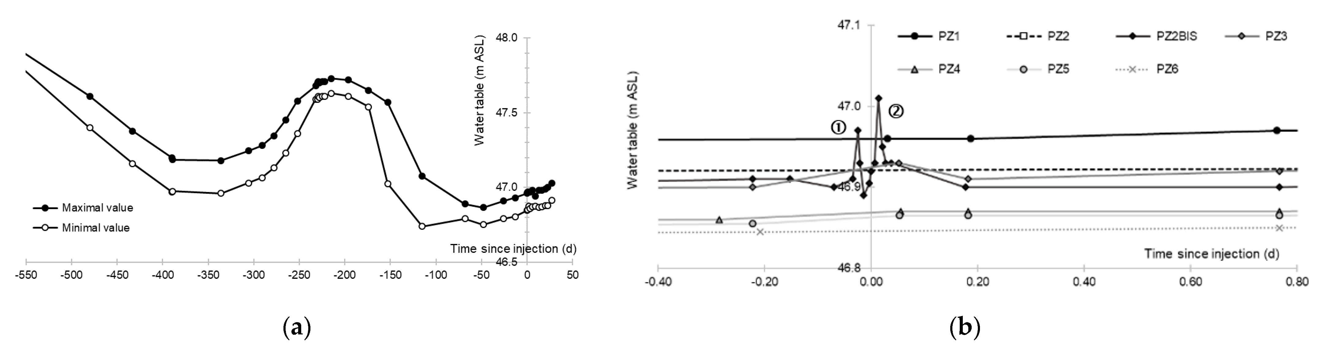
3.1. Aquifer Piezometry

Long-term piezometric monitoring was set up more than a year before injection [6]. During the 2019–2020 hydrological cycle, the average water table of the site reached its maximum in mid-April 2019 with 47.67 m ASL and its minimum at the beginning of October 2019 with 46.80 ASL (Figure 8a). Since that date, i.e., 49 days before the experiment, the piezometric level rose regularly as a result of the autumn recharge.

During the injection, the average piezometric level of the site remained stable at 46.90 m ASL, with the exception of PZ2BIS (+0.07 m) and PZ3 (+0.03 m), which were affected by the injections (Figure 8a). This was probably also the case for PZ2TER, located between the two previous piezometers, but it was not possible to measure its water table due to the presence of a packer.

At PZ2BIS, a first piezometric peak of +0.07 m occurred 0.25 h after the start of the first injection (see circled 1 in Figure 8b), and then the water table returned to its original level just before a new peak of +0.11 m, which occurred 0.33 h after the start of the second injection (see circled 2 in Figure 8b). The water table returned to its initial state 2 h after the end of the second injection. This piezometer was therefore influenced by the average overpressures of 1.4 bar induced by the successive injections and, to a lesser extent, same for the PZ2TER and the PZ3.

3.2. Tracing of the Injected Water

PZ2 remained sealed for 24 h after the injections to limit the risk of hydrogen degassing. When it was reopened, despite the leaching induced by the injection of 5 m³ of hydrogenated water that followed the injection of 1 m³ of tracer-holding water, the tracer concentrations still reached 208 µg·L⁻¹ for lithium, 117 µg·L⁻¹ for uranine, and 3.9 µg·L⁻¹ for helium (Figure 9). Depending on the tracer, this represents 0.3–2% of the concentration injected the day before. Since the injection induced an overpressure, this phenomenon is probably due to the retention of part of the tracers within the chalk’s porous matrix (which is of micrometric dimension), and then to their slow release when the natural flow of the aquifer resumed. This phenomenon has previously been demonstrated at other sites where the chalk shows dual porosity [29,30]. Thus, in the injection well, the tracer concentration remained higher than the background noise for 12.9 days for lithium and helium and until the end of the monitoring (t ≥ 49.9 days) for uranine, on which date the analyses still showed the presence of 0.29 μg·L⁻¹ of this tracer. This retention phenomenon therefore generated a decreasing but clearly significant background noise for about two weeks after injection.

At PZ2BIS, 5 m downstream, three successive tracer plumes were observed (Figure 10b):

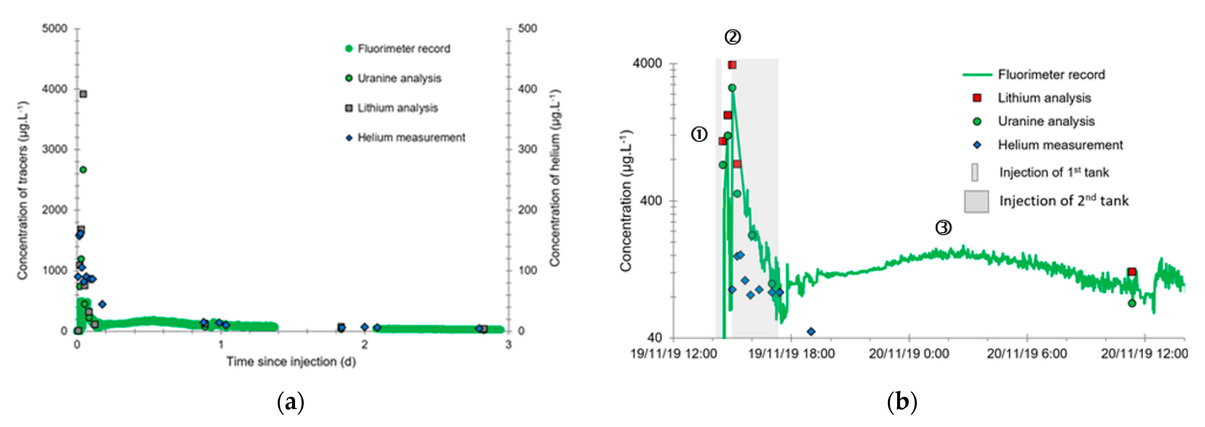
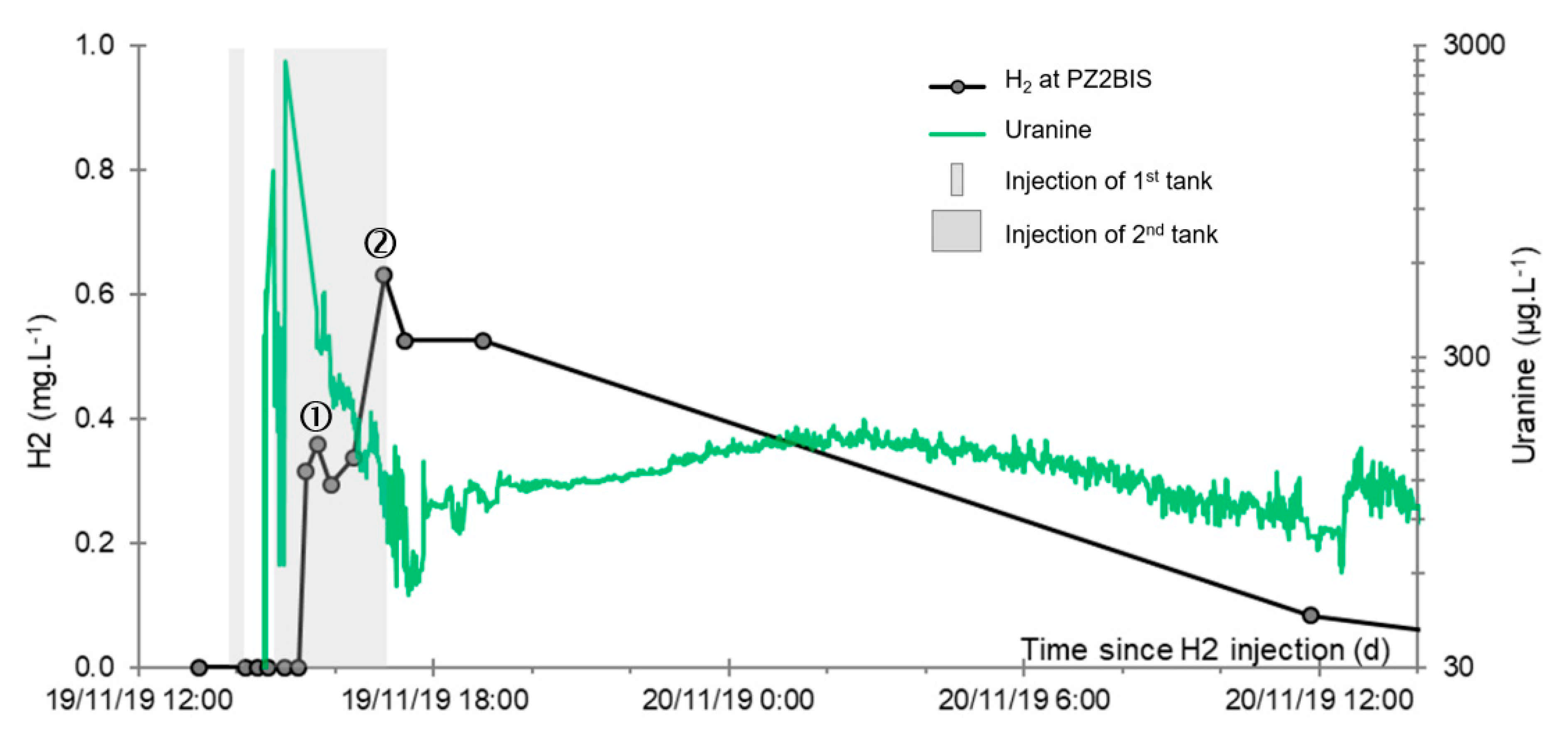
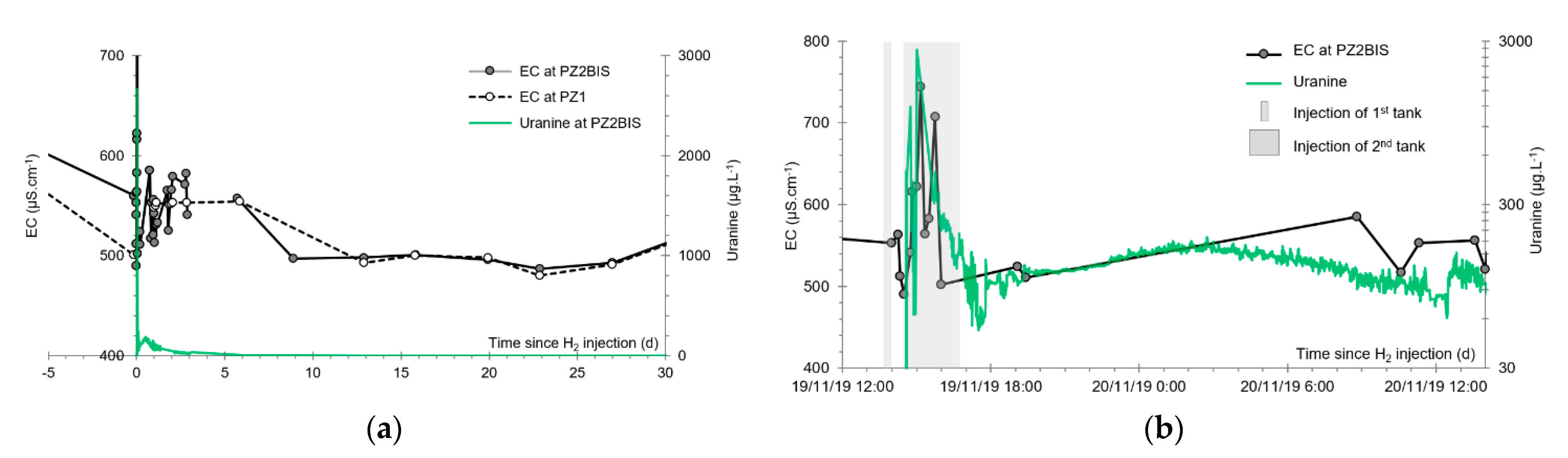
• A first plume caused a significant peak (see circled 1 in Figure 10b). It started at 14:30, i.e., 0.5 h after injection of the tracers, and peaked at 14:45 at a concentration of 1678 µg·L⁻¹ for lithium and 1188 µg·L⁻¹ for uranine (a signal which saturated the fluorimeters). Due to an initially inadequate measurement interval scheme, no helium was detected in this first plume that corresponds to the passage of water from the tracer tank. During this peak, which lasted approximately 1 h, the tracer concentration reached 17% of the lithium injection concentration and 12% of the uranine injection concentration, i.e., a dilution factor of 5.96 and 8.42, respectively.
• A second more intense and longer plume lasted about 3.5 h, synchronous with the injection of the hydrogenated water (see circled 2 in Figure 10b). It peaked at 15:00, i.e., approximately 10 min after the start of injection, at a concentration of 3913 µg·L⁻¹ for lithium, 2667 µg·L⁻¹ for uranine (again inducing saturation of the fluorimeters), and 160 µg·L⁻¹ for helium. The tracer dilution factors reached 2.56, 3.75, and 9.28, respectively. This plume is interpreted as the result of leaching of the tracers contained in the porous matrix of the aquifer rock induced by the arrival of water at a slight overpressure from the second tank.
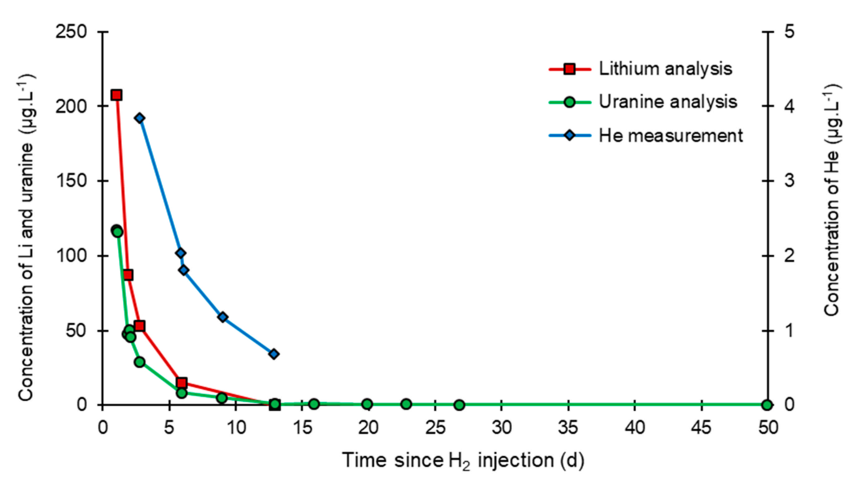
• In the third, weaker and more spread-out plume (see ③ in Figure 10b; note the logarithmic axes), uranine was detected by the fluorimeter. It peaked at 189 µg·L⁻¹ on 20 November 2019 at 02:45 (t = 0.531 days) and decreased very slowly, finally lasting about a month; 0.24 µg·L⁻¹ of uranine remained at t = 26.8 days, lithium and helium having disappeared by t = 12.9 days. When the concentration peak passed through, the dilution factor reached 52.9 for uranine, the only tracer measured using the recording fluorimeter (because the peak occurred in the middle of the night), which must have corresponded to a dilution factor of about 36 for lithium and about 130 for helium.

As regards the other downstream piezometers, a peak of tracers is clearly noticeable at PZ3 (10 m downstream) and PZ4 (20 m downstream) at t = 2 days with respective concentrations of 9.75 and 9.08 µg·L⁻¹ for uranine (Figure 11a). These peaks seem to be shifted to t = 6 days for lithium with respective concentrations of 15 and 10 µg·L⁻¹ (see circled 1 in Figure 11b), and for helium with respective concentrations of 1 and 2 µg·L⁻¹ (Figure 11c). At PZ4, a second lithium peak is also observed at t = 20 days with a maximum concentration of 24 µg·L⁻¹ (see circled 2 in Figure 11b). This distinct behavior of piezometers PZ3 and PZ4 has been observed previously. It means that the tracers arrive as quickly and at the same concentrations at PZ3 as at PZ4, which is twice as far from the injection well, with respective speeds of 5 and 9.5 m·day⁻¹. It is assumed that the groundwater takes a dual flow path, which is more marked at PZ4 than at PZ3, with a rapid circulation within a more permeable (probably fissured) zone, and a slow circulation within the aquifer’s porous matrix.

Regarding the piezometers located far downstream, namely PZ5 at 30 m and PZ6 at 60 m, traces of each of the two tracers are observed there approximately two weeks after injection (about 0.6 µg·L⁻¹ for uranine, about 10 µg·L⁻¹ for lithium), and helium is detected six days after injection with a concentration lower than 1 µg·L⁻¹ (Figure 11a). Although the peak concentration of tracers has not yet been reached when the monitoring was stopped, it can be estimated that the corresponding transfer rates here are less than 1–2 m·day⁻¹. The dilution ratio is from 0.01% to 0.1%, which means that the impact of the hydrogen injected into the aquifer cannot be measured at these distances, under the experimental conditions created. Note that this result is in line with that obtained by PHREEQC modeling during the previous helium injection test [6].

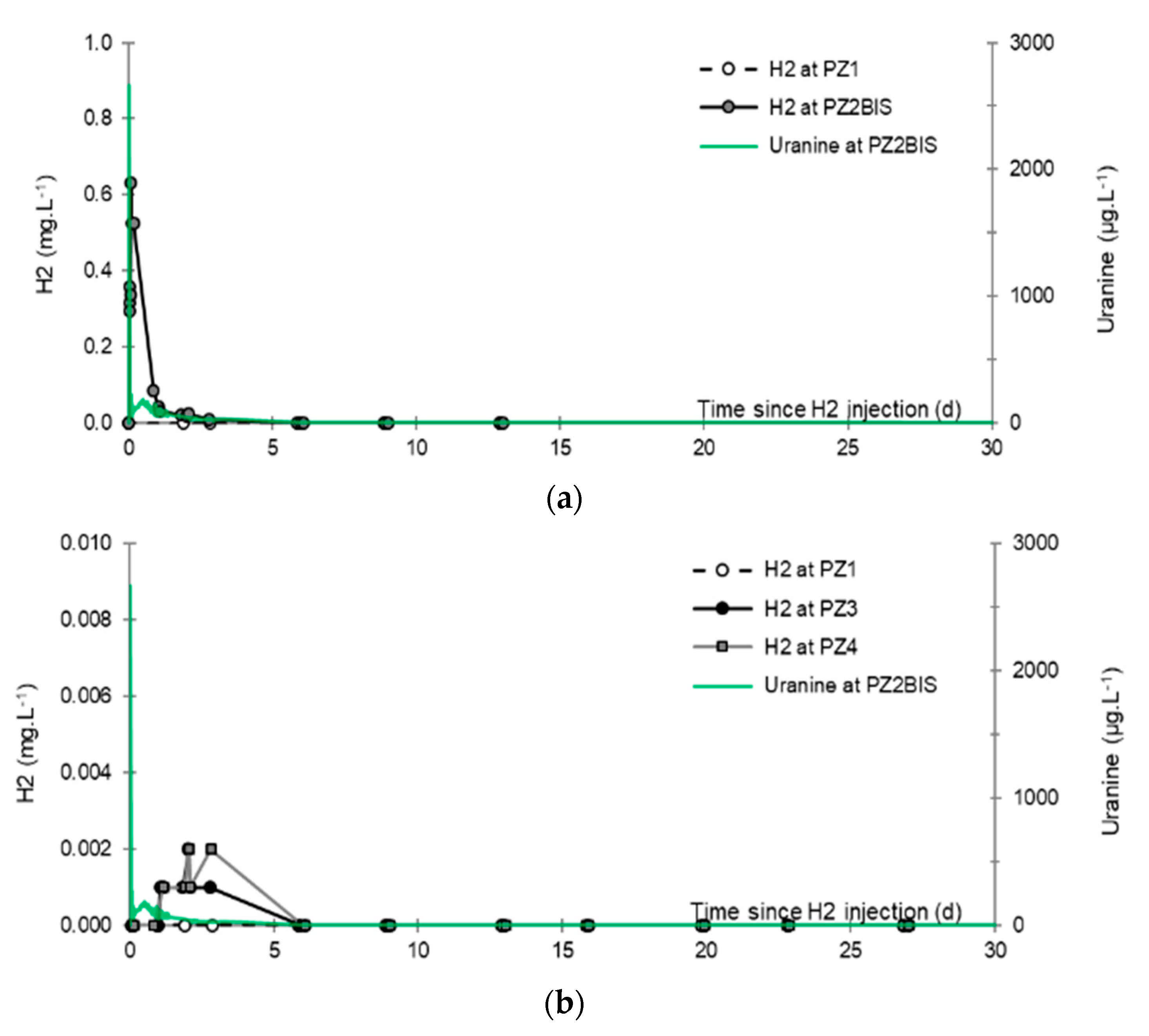
3.3. Dissolved Hydrogen

In the water samples obtained by pumping, the dissolved hydrogen is extracted by the method of partial degassing by mechanical agitation, after which its content is measured with a portable Biogas analyzer with a detection threshold of 0.5 µg·L⁻¹. The dissolved CH₄ and H₂S are also measured by the same method, with respective detection limits of approximately 1 and 0.6 µg·L⁻¹. In parallel, the gases dissolved in the water of the PZ2TER are analyzed by Raman and Infrared spectrometry [25].

The results obtained are as follows (Figure 12):

• No trace of dissolved CH₄ or H₂S is detected in any piezometer using the method of partial degassing by mechanical agitation.
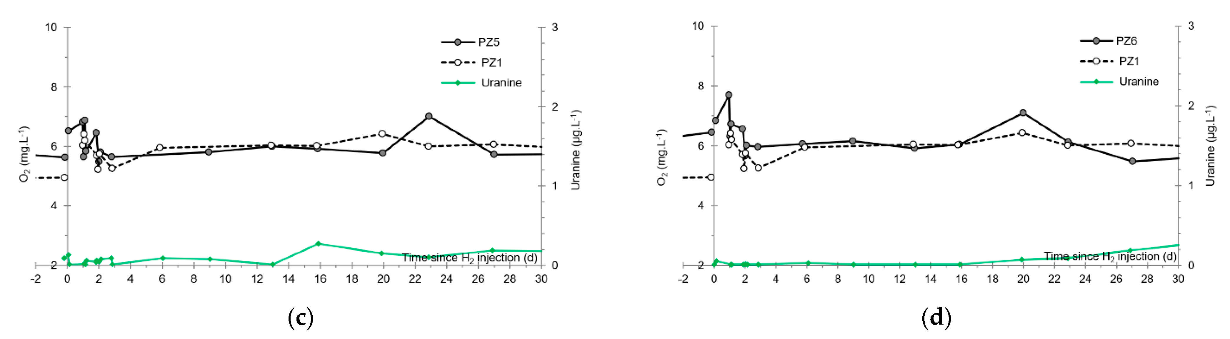
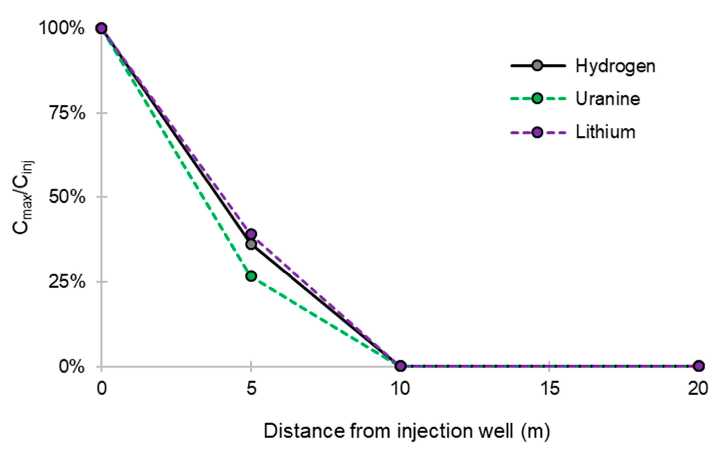
• No trace of dissolved H₂ is detected at PZ1 located 20 m upstream of the injection well or at PZ5 and PZ6, respectively, located 30 and 60 m downstream of the injection well.
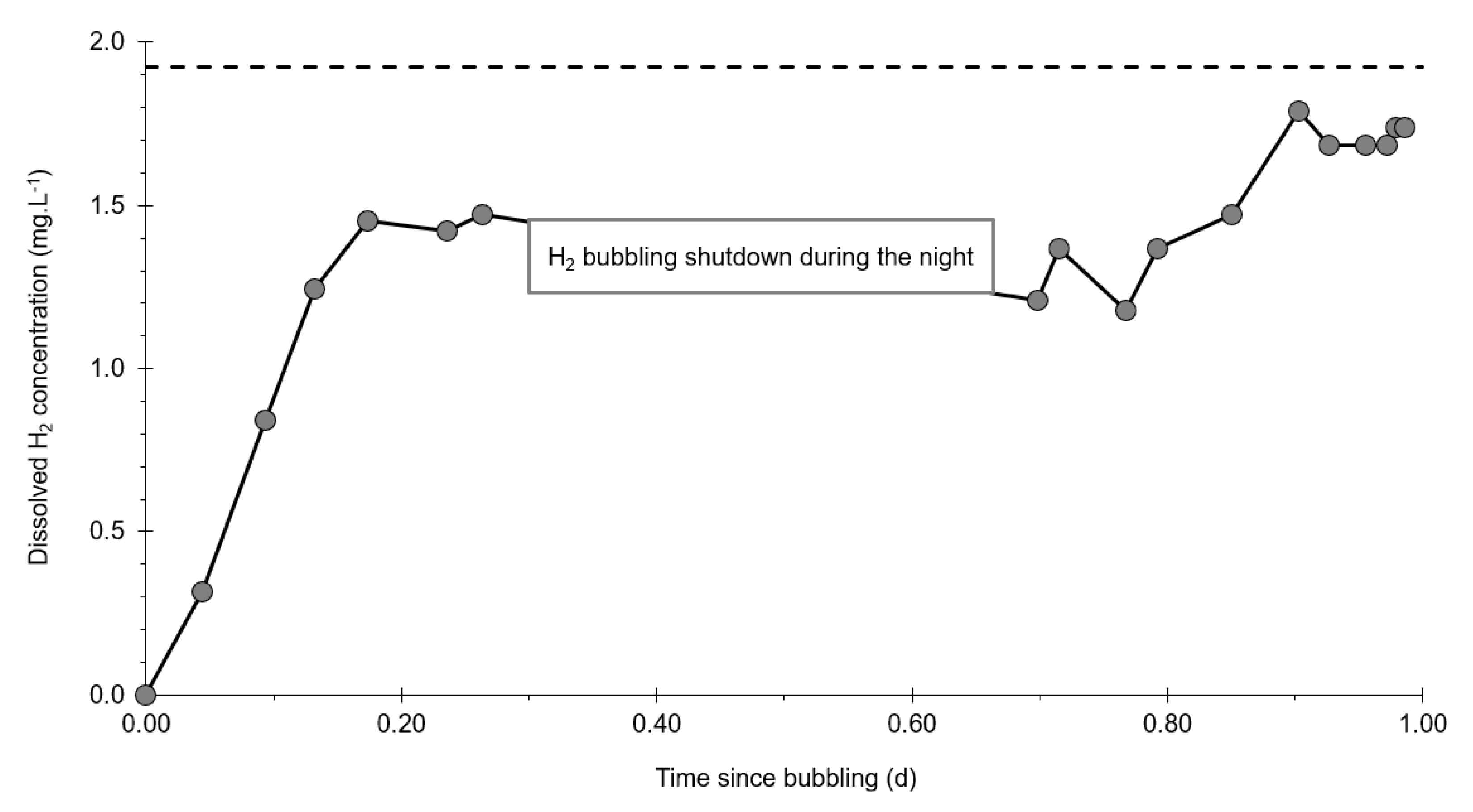
• At the injection well (PZ2), the dissolved H₂ concentration, which is 1.76 mg·L⁻¹ at the time of injection, is still 0.084 mg·L⁻¹ when the well was reopened, i.e., 1.8 days after the start of the injection. This residual concentration represents 5% of the concentration of the injected water.
• At the main monitoring piezometer (PZ2BIS), located 5 m downstream, the concentration peak passed 2 h after the injection started (i.e., 0.08 days) with a value of 0.63 mg·L⁻¹. This corresponds to a theoretical transfer velocity of 60 m·day⁻¹ what is not a representative value of the mean transfer velocity of the water in the aquifer (which is approximately 3–10 m·day⁻¹ according to Gombert et al. [7]) because it is strongly influenced by the injection.
• At the monitoring piezometer PZ2TER located 7 m downstream, the dissolved H₂ concentration peak detected by Raman spectrometry passed through 9.7 h after the start of injection (i.e., 0.40 days) with a value of 0.17 mg·L⁻¹ [25]. This corresponds to a theoretical transfer velocity of 17 m·day⁻¹; value still strongly influenced by the injection.
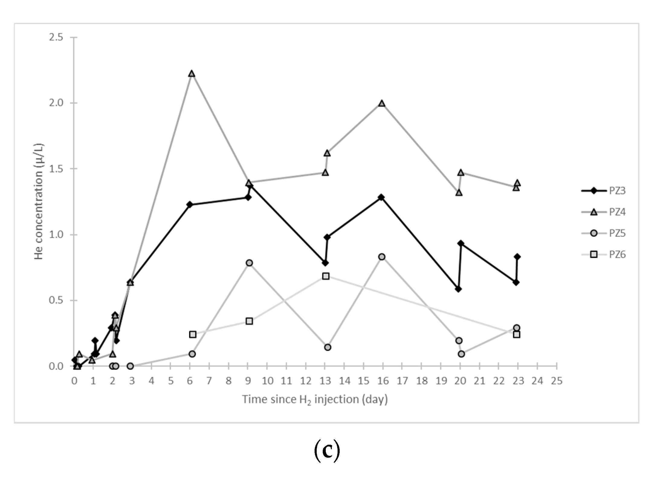
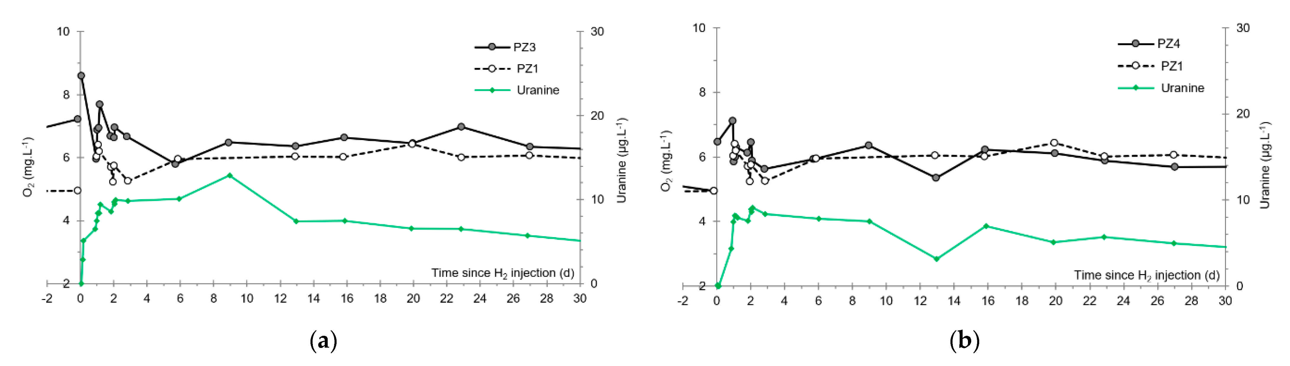
• At the PZ3 piezometer, located 10 m downstream, the first traces of dissolved H₂ appeared at 1.05 days and the concentration reached its maximum of 1.7 µg·L⁻¹ after 2.02 days, which corresponds to a transfer velocity of 5 m·day⁻¹.
• At the PZ4 piezometer, located 20 m downstream, the first traces of dissolved H₂ appeared at 1.2 days and the concentration peaked a first time at 1.5 µg·L⁻¹ after two days and a second time at 1.74 µg·L⁻¹ after 2.8 days. This corresponds to transfer speeds of around 10 and 7 m·day⁻¹, respectively.

A detailed analysis of the evolution of the dissolved hydrogen concentration at the main monitoring piezometer PZ2BIS during the injection day shows that the first peak appears only 38 min after the start of the hydrogenated water injection at 0.36 mg·L⁻¹ (see circled 1 in Figure 13), following which a second more significant peak reaching 0.63 mg·L⁻¹ occurred after 2 h (see circled 2 in Figure 13). These two peaks occurred during the injection of hydrogenated water, which lasted 2.5 h. Thus, at this close distance to the injection well, PZ2BIS appears to be strongly disturbed by the experimental conditions and particularly the overpressure induced. Similar to the tracers, the theoretical transfer speed it provides is not representative of the natural flow of the aquifer water, but instead of a flow disturbed by the successive injections.

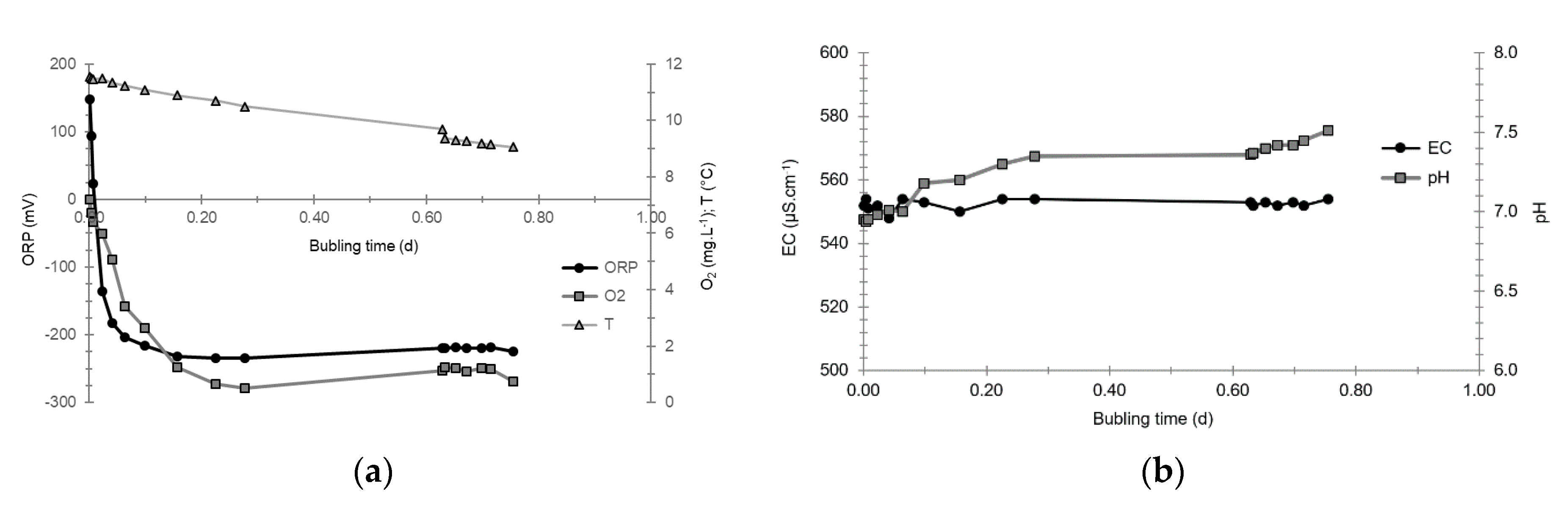
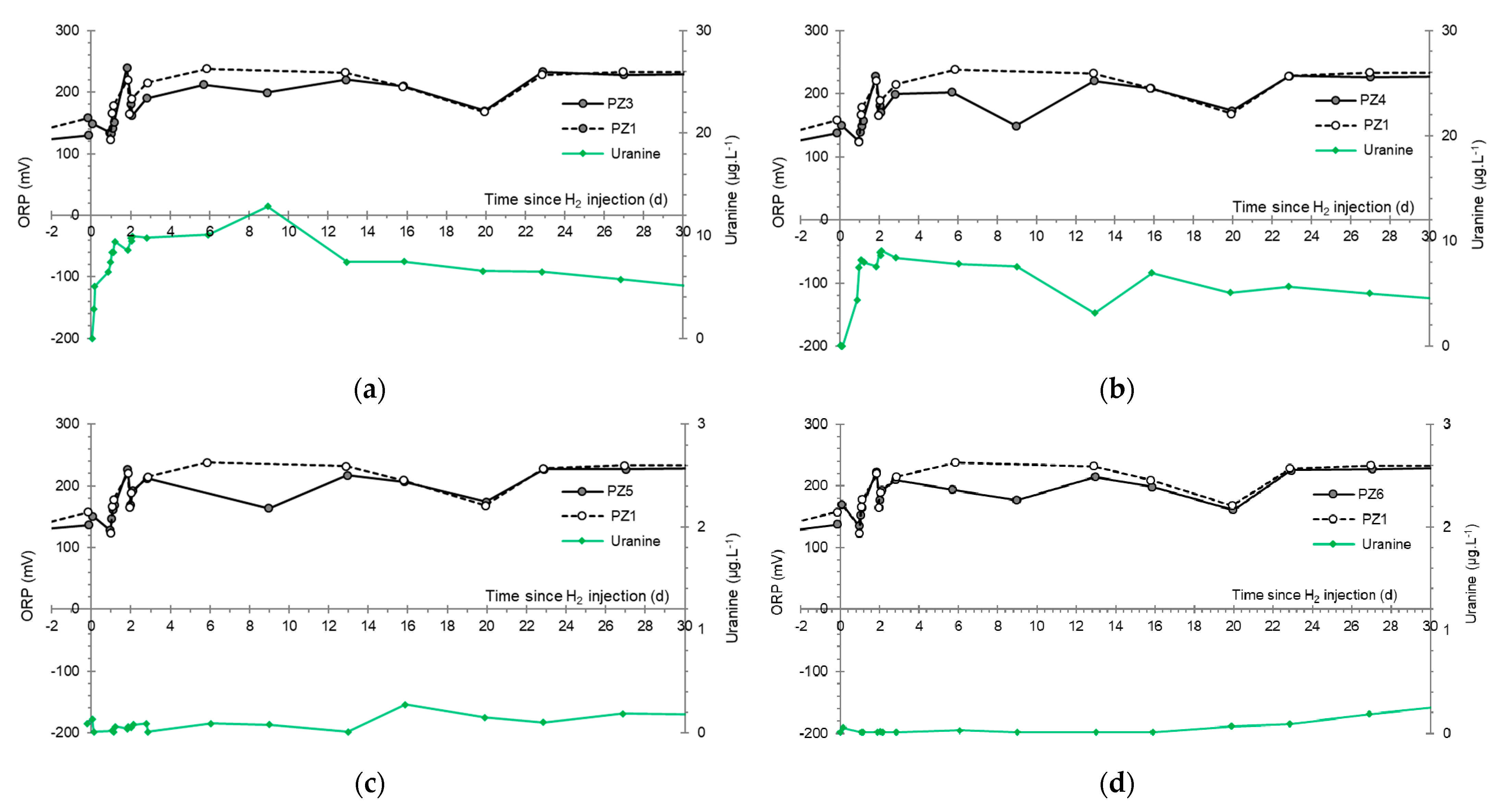
3.4. Oxidation-Reduction Potential

At the PZ2 injection well, the baseline showed an average oxidation-reduction potential of +192 mV prior to the injections [6]. When the measurements are resumed with the reopening of the well the day after the injections (t = 1.01 days), the oxidation-reduction potential is still low, with a value of +94 mV and it did not regain its initial value until t = 2.8 days onwards (Figure 14a).

At PZ2BIS, the oxidation-reduction potential decreased from +154 mV prior to the injections to a minimum of −139 mV during the injection (Figure 14b).Despite the shift in the values due to a difference in the calibration of the measuring probes, it is noted that the water remained reductive for at least 1.8 days and did not return to its normal value until after 2.8 days.

Again, at PZ2BIS, a detailed examination of the first day of the experiment shows the existence of two successive minima (see circled 1 and 2 in Figure 15):

• The first is not very marked (−22%) and reached +120 mV at 14:15, i.e., 15 min after injection from the first tank containing helium and hydrological tracers. It corresponds to the passage of less oxidizing water, probably because of its deoxygenation induced by the introduction of dissolved helium.
• The second is very clear (−190%) and it reached −139 mV at 15:45, i.e., 55 min after injection from the second tank containing dissolved hydrogen. This drop is in fact synchronous with the second tracer peak.

Due to the persistence of reducing conditions in the aquifer, in particular because of the release of the hydrogenated water stock present in the chalk’s porous matrix in the immediate surroundings of the injection well, the oxidation-reduction potential remained at low values for the first day after the injection at PZ2BIS. It then increased in regular fashion at a mean speed of +59 mV·day⁻¹ as a result of three mechanisms acting in unknown proportions: (i) dilution of the plume injected into the aquifer; (ii) partial degassing of the hydrogen; and (iii) potential chemical or biochemical reaction between the hydrogen and certain elements present in the water or the aquifer rock.

For the piezometers located further downstream, we consistently noted the existence of fluctuations in the oxidation-reduction potential during the first two days (Figure 16). These are in fact artifacts arising from the increased frequency of measurements, which demonstrate intraday fluctuations that were not visible during the looser monitoring on the other days. Apart from this, there is no evidence of an impact of the injection of hydrogenated water on the oxidation-reduction potential once the distance downstream of the injection well reaches 10 m.

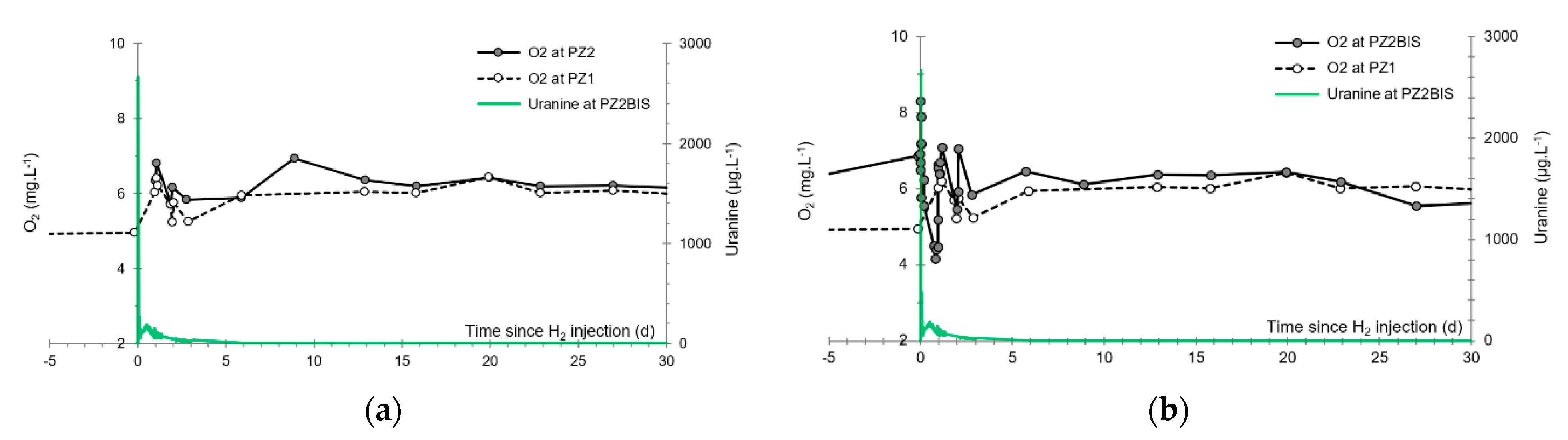
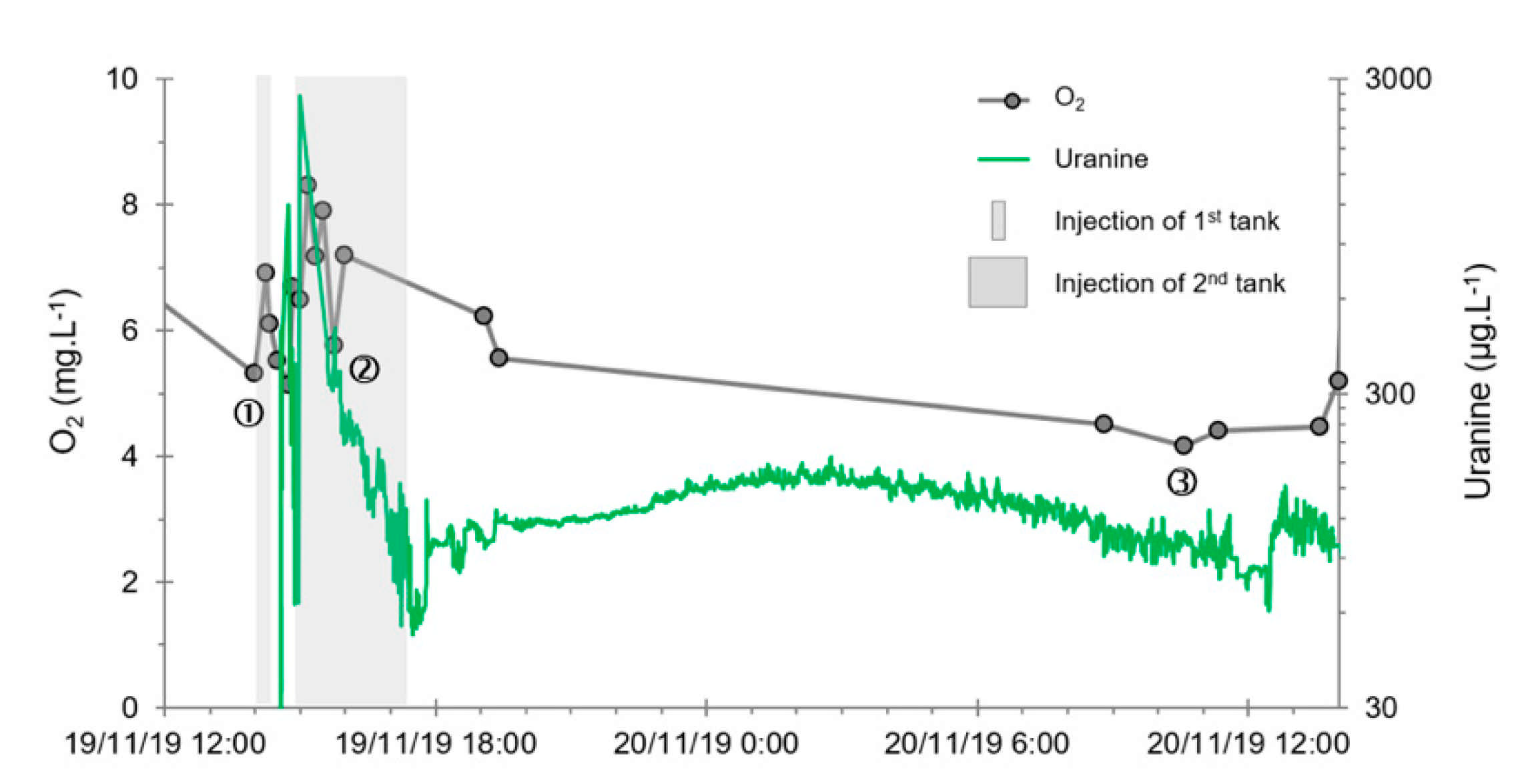
3.5. Dissolved Oxygen

At the PZ2 injection well, the mean concentration of dissolved oxygen during baselining equaled 6.30 mg·L⁻¹ [6]. The day after the injections, the first measurement taken at 6.27 mg·L⁻¹ has the same order (Figure 17a) of magnitude. This shows that the impact of the injection on this parameter is already no longer visible at this point.

In contrast, at PZ2BIS, the mean concentration dropped from 6.24 mg·L⁻¹ prior to the injections to a minimum of 4.17 mg·L⁻¹ at t = 0.82 days (Figure 17b). As with the oxidation-reduction potential, there are also significant fluctuations in the dissolved oxygen concentration during the first two days following the injections, probably also linked to the increase in the frequency of measurements and the disturbances induced by operations at the piezometers.

A detailed inspection of the first day of the experiment clearly shows the existence of three successive minima on 19 November 2019 at 14:45 with 5.13 mg·L⁻¹, on 19 November 2019 at 15:45 with 5.77 mg·L⁻¹, and on 20 November 2019 at 10:35 with 4.17 mg·L⁻¹ (Figure 18):

• The first one, synchronous with the first tracer peak, corresponds to the passage of water from the first tracer tank (see circled 1 in Figure 18). This water is deoxygenated due to the bubbling of helium.
• The second one, synchronous with the second tracer peak, corresponds to the rapid passage of water from the second tank. This water is deoxygenated due to the bubbling of hydrogen (see circled 2 in Figure 18).
• The third one, synchronous with the third tracer peak, corresponds to the slow passage of water from the second tank (see circled 3 in Figure 18). It signals the arrival of the main plume of hydrogenated water, which circulated more slowly within the aquifer and still contained under-oxygenated water for about a day after the injections.

Regarding the other piezometers located further downstream, fluctuations are systematically noted during the first two days of monitoring with dissolved oxygen concentrations below 6 mg·L⁻¹: this is also considered as an artifact associated with the higher frequency of measurements (Figure 19). Apart from these fluctuations, as the distance downstream of the injection well approaches 10 m, there is no evidence of an impact due to the injections on the dissolved oxygen concentration in the water.

3.6. Other Physicochemical Parameters

Regarding the electrical conductivity, we note the existence of natural variations within the aquifer, recorded at PZ1 upstream of the injection well: at this piezometer, before injection and up to six days after, the average conductivity is 550 µS·cm⁻¹; it then decreases to 492 µS·cm⁻¹ after this date. This fluctuation, which is observed upstream of the area affected by the injections, therefore affects the entire aquifer with successive repercussions on all piezometers: at PZ2BIS, the conductivity thus dropped from 558 to 495 µS·cm⁻¹ (Figure 20a). On the other hand, a detailed analysis of the first day following the injection again shows the same three successive decreases in concentration already encountered at this piezometer with the previous physicochemical parameters (Figure 20b). The minimal values are reached on the day of injection at 14:30 with 490 µS·cm⁻¹, at 15:20 with 564 µS·cm⁻¹, and at 16:00 with 502 µS·cm⁻¹. As before, this corresponds to the rapid passage of the plumes of water from the two tanks, as well as the slow release into the aquifer of water that has remained trapped in the porous matrix around the injection well.

We show below that this correspond mainly to a decrease in the cumulative concentration of the dominant ions (Ca²⁺, Mg²⁺, and HCO₃) of this bicarbonate-calcic groundwater: this is interpreted as a consequence of the precipitation of CaCO₃ and MgCO₃ from the degassing of dissolved CO₂ following the saturation of the water with He or H₂. On the other hand, these decreases are immediately followed by a peak in conductivity reaching 744 µS·cm⁻¹ for the first, 707 µS·cm⁻¹ for the second, and, later (t = 2.80 days), 582 µS·cm⁻¹ for the third. These are the highest values recorded since the implementation of baseline monitoring over more than a year ago. These cycles of decrease and increase should therefore be related to the injections conducted: it seems that the observed increases can result from the dissolution of the carbonaceous aquifer rock by the injected water, which became aggressive to calcite, following the degassing of CO₂ induced by the bubbling with other gases.

Regarding pH, we note that it is already varying cyclically from 6.8 to 7.4 at PZ1 (upstream) before the injections. As is the case for the conductivity, we assumed that these are natural groundwater fluctuations since they are measured upstream of the injection well, and they affect the entire experimental site up to the most downstream piezometers: at PZ2BIS, the pH thus varies from 7.0 to 7.7 (Figure 21a). On the other hand, the detailed analysis of the first day following the injection shows, at this piezometer, a weak but sudden increase in pH from 7.2 to 7.4 when the first two tracer peaks passed through (Figure 21b). This behavior is to be linked to the degassing of dissolved CO₂, following the dissolution of He and H₂. The pH then decreased to 6.9 after t = 2.88 days, i.e., for the duration of the passage of the third plume of water, while at the same time the water at PZ1 showed an increase of natural origin. One could possibly interpret this increase as an impact of the slow arrival of hydrogenated water with the main aquifer flow.

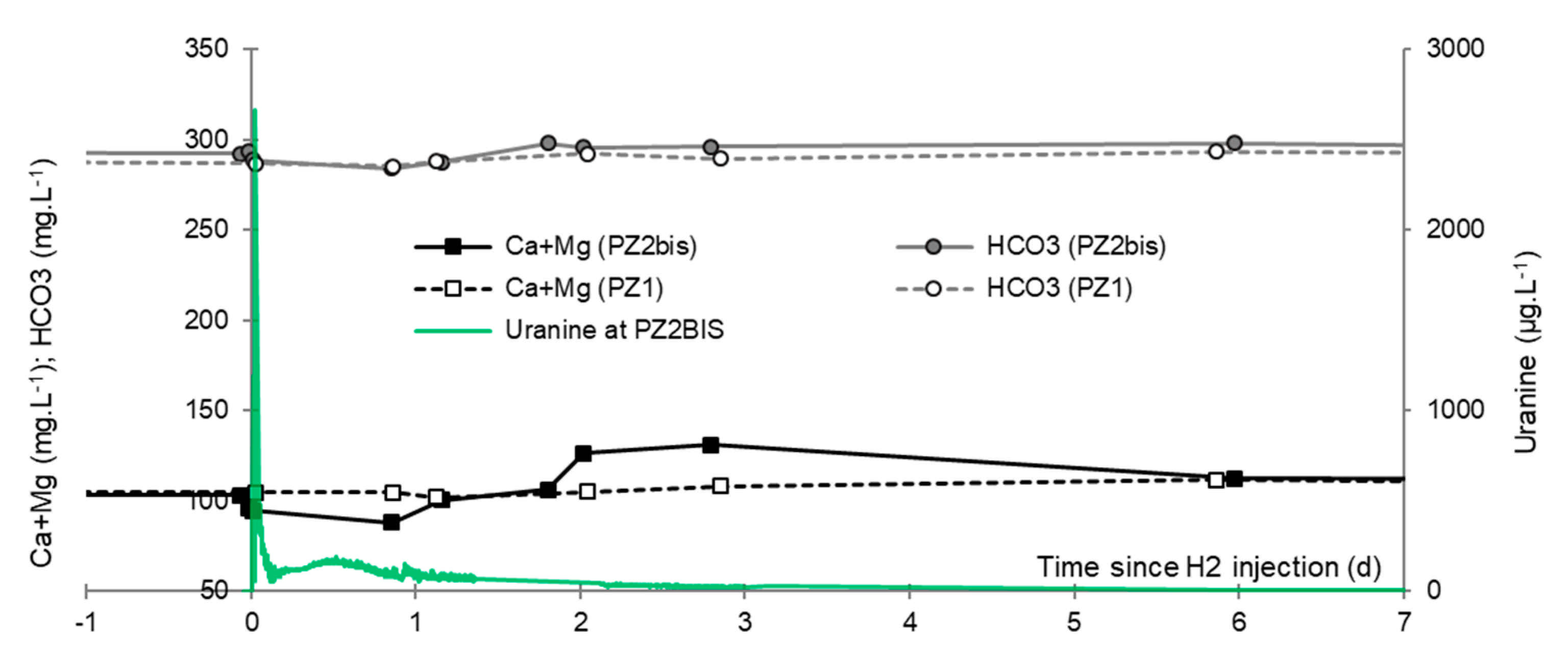
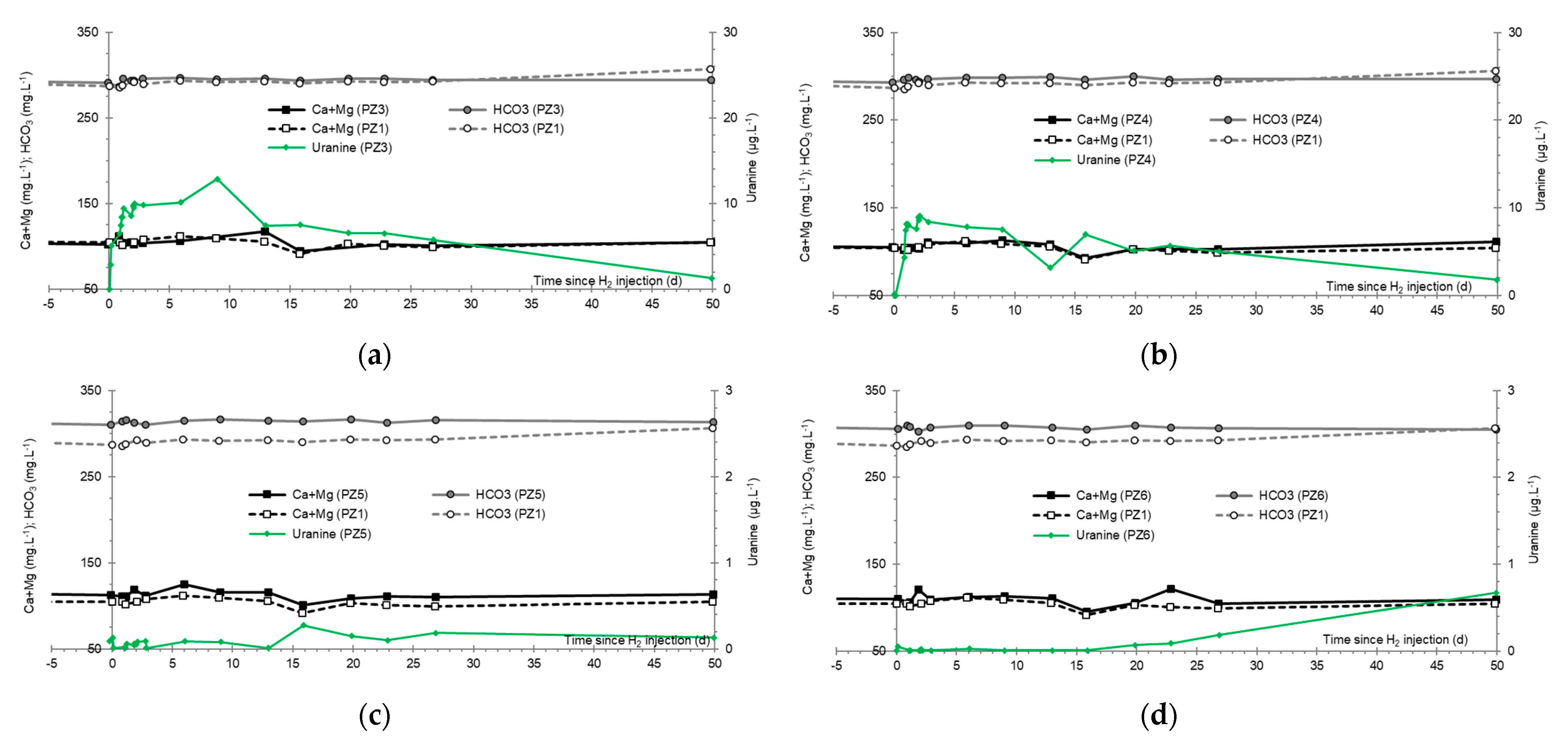
3.7. Dominant Ions (Ca²⁺, Mg²⁺ and HCO₃⁻)

The saturation of the water in the first tank with helium and then that of the second tank with hydrogen caused the degassing of the natural gases initially present, mainly an admixture of CO₂, N₂, and O₂. The degassing of CO₂ notably upsets the calco-carbonic equilibrium in the water, which seems to have led to the precipitation of CaCO₃ at the bottom of the tanks and MgCO₃ to a lesser extent, totaling a probable loss of around 29 mg·L⁻¹ of dissolved elements. The water injected into the aquifer is therefore undersaturated with calcite and dolomite, which explains the observed decrease in the concentrations of Ca²⁺, Mg²⁺, and HCO₃⁻ in the samples taken during the first day (Figure 22). The cumulative concentration of these three ions decreased from 401 mg·L⁻¹ before injection to a minimum of 372 mg·L⁻¹ during injection, which corresponds to a 9.1% drop in their molar concentration shortly after the passage of the injected plumes. A maximum of 427 mg·L⁻¹ is then observed at t = 2.80 days. This is interpreted as the dissolution of the carbonaceous aquifer rock by the injected water, which became more aggressive with respect to calcite and dolomite. The concentrations then reached their normal baseline values between the third and sixth days, with a cumulative concentration of 405 mg·L⁻¹ until the end of monitoring.

These cycles of variations in concentrations does not appear at any of the piezometers located further downstream (Figure 23). This shows that the aquifer has already returned to its natural calco-carbonic equilibrium at a distance of 10 m downstream from the injection well.

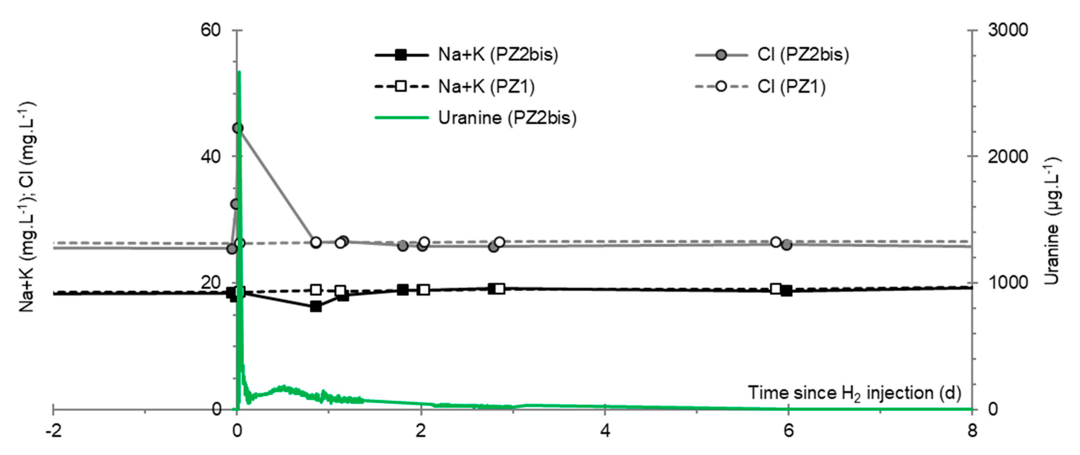
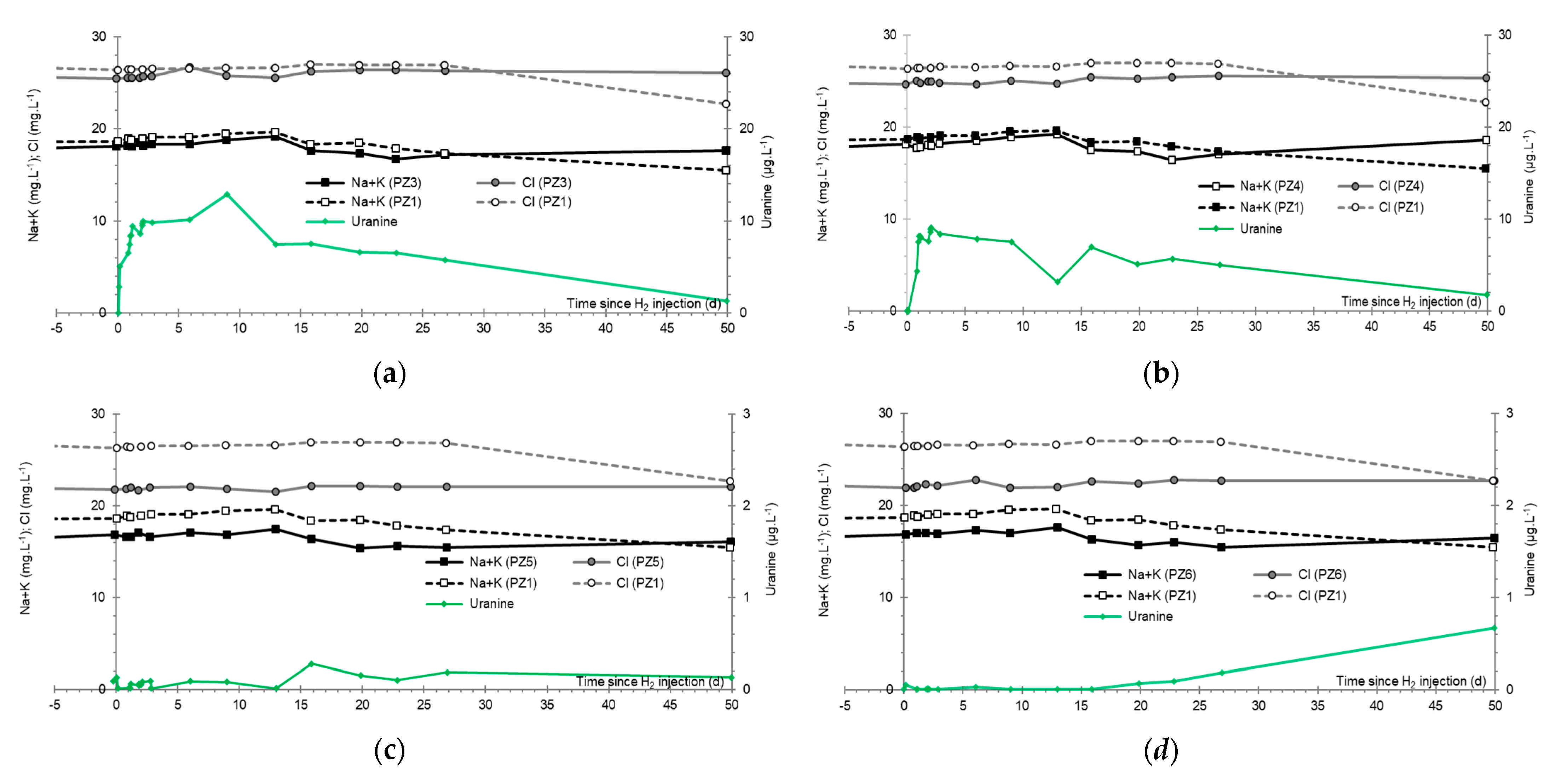
3.8. Chlor-Alkali Ions (Cl⁻, Na⁺, and K⁺)

We observed a quasi-stability of the cumulative concentration of alkaline ions (Na⁺ and K⁺) at around 18.0 mg·L⁻¹, while the concentration of Cl⁻ increased very significantly shortly after the injection of the water with tracers (Figure 24): it rose from 25.0 mg·L⁻¹ before injection to 32.5 mg·L⁻¹ from the moment of tracer injection and then peaked at 44.5 mg·L⁻¹ before dropping again and stabilizing at 26.0 mg·L⁻¹.

The first sample in which an increase is detected is taken before the injection of hydrogen, but 0.50 h after the injection of the tracers. It is therefore an artifact caused by the presence of an ionic tracer, the lithium ion, in the form of lithium chloride (LiCl). This tracer was added to the water in the first tank in order to achieve a Li⁺ ion concentration of 10 mg·L⁻¹, which also represents an additional Cl⁻ ion concentration of 51.4 mg·L⁻¹.

As previously, this excess of chloride ions is no longer observed at the piezometers located further downstream, i.e., beyond 10 m from the injection well (Figure 25).

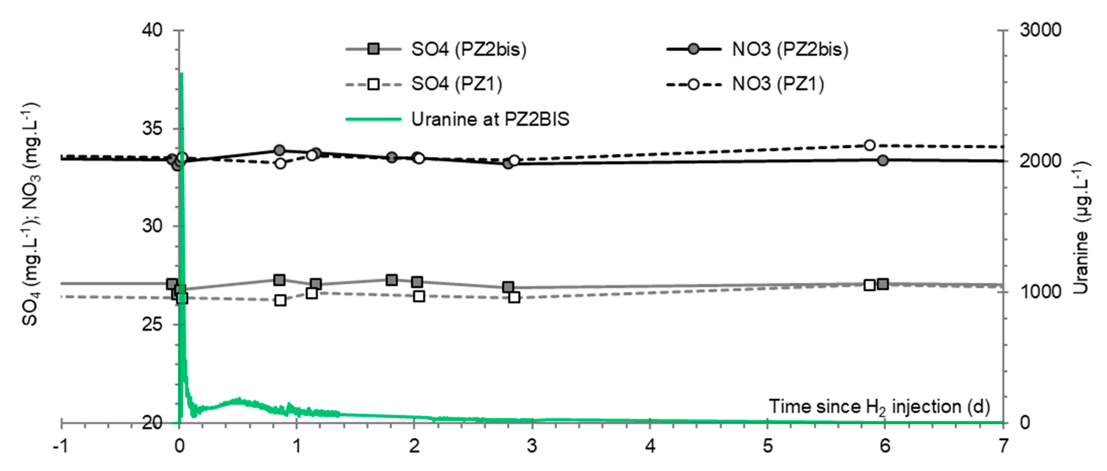
3.9. Nitrates, Sulfates, and Their Derivatives

Nitrates and sulfates are oxidized ions which are potentially reactive to the presence of hydrogen: they are in fact liable to be reduced to nitrites or ammonium ions for the former and sulfides or sulfites for the latter, particularly in the presence of metal catalysts.

Figure 26 shows that the sulfates do not seem to have been affected during injection. At PZ2BIS, their concentration remained stable at 26.9 mg·L⁻¹, a value corresponding to that of the PZ1 upstream piezometer (27.0 mg·L⁻¹). The same behavior is observed at the other piezometers located further downstream of the injection well. On the other hand, there is no trace of sulfides or sulfites above their analytical detection limit of 0.01 mg·L⁻¹. There is therefore no evidence of a reactivity of the sulfates to the injection of hydrogen under the conditions of the experiment. It is noted that the tubing of all the piezometers is made of PVC or HDPE and no metallic item likely to act as a catalyst came into contact with the aquifer.

Figure 26 also shows that the nitrates do not seem to have been affected during injection. Their concentration at PZ2BIS remained stable at 33.3 mg·L⁻¹, a value corresponding to that of the PZ1 upstream piezometer (33.9 mg·L⁻¹), and there is no trace of nitrites above their analytical detection threshold (0.01 mg·L⁻¹). On the other hand, the ammonium ions exhibited cyclic fluctuations during monitoring, but this is detected at all the piezometers, including the one located upstream of the injection well (Figure 27). Before the injection of hydrogenated water, therefore, there are already traces of ammonium ions at all piezometers at an average concentration of about 0.10 mg·L⁻¹. These ions could be either the residues from the application of ammoniacal fertilizers or the result of a weak natural denitrification. It is recalled that, since the well’s tubing is not metallic, it cannot act as catalysts for a possible denitrification linked to hydrogen injection.

4. Discussion

Panfilov [3] pointed out in 2015 that few articles have been published on the scientific aspects of hydrogen behavior in geological structures. Since then, studies on the impact of hydrogen leaks in an aquifer are still very rare. These include the experimental laboratory work of Berta et al. [22] and an ongoing experiment by the same team at the University of Kiel (D) on a shallow aquifer, the results of which have not yet been published. The results obtained by Berta et al. [22] are however not extrapolatable to our case: they concerned a long contact period (six months) between hydrogen under pressure (2–15 bars) and a reconstituted aquifer medium. Under these specific conditions, the reduction of sulfates, the production of acetate, the precipitation of calcite, and, consequently, an increase in pH and a decrease in electrical conductivity were observed. These parameters were considered as potential targets of a monitoring network covering a hydrogen gas storage site. However, it has been shown that these modifications resulted from the development of a hydrogenotrophic microbial community including sulfate-reducing bacteria.

In our experiment, several physicochemical and hydrogeochemical phenomena occurred in the hydrogen saturation tank, and then, following the injection of the hydrogenated water, at the piezometers near downstream to the injection well. Some of these phenomena are the result of the injection of hydrogenated water (drop in the redox potential dissolved hydrogen in water), but some others are the results of the preliminary dissolution of helium and tracers (mainly, deoxygenation of water and degassing of CO₂). At PZ2BIS, the main monitoring piezometer located 5 m downstream to the injection well, such variations are synchronous with the passage of the first uranine peak (fluorescent tracer), which signaled the arrival of the hydrogen-free (helium-saturated) water from the first tank. Once injected into the aquifer, this first water therefore caused the same phenomena as those observed in the tank, but at a lower intensity as a result of its dilution: A drop in the oxidation-reduction potential, the dissolved O₂ concentration, the electrical conductivity and the concentration of dominant ions (Ca²⁺, Mg²⁺, HCO₃⁻). In addition, the water from this tank also contained an excess of Cl⁻ ions, linked to the presence of LiCl as an ionic tracer: it thus caused an increase of Cl⁻ ions in the aquifer. Since this ion is particularly conservative, it makes it possible to calculate that the dilution factor of the first injected plume must have reached 60% during the passage of the tracer peak at this piezometer.

The dissolution of hydrogen in the second tank also resulted in the same phenomena related to the degassing of dissolved O₂ and CO₂: the dissolved O₂ concentration dropped and the pH increased as a result of the degassing of dissolved CO₂. This must have also induced the precipitation of some of the dominant ions (Ca²⁺, Mg²⁺ and HCO₃⁻) in the water of the tank. The presence of dissolved hydrogen at a concentration close to saturation, additionally caused a significant drop in the oxidation-reduction potential, which made the water in this tank highly reducing: this is the only real impact directly linked to the saturation of water with hydrogen. Shortly after its injection into the aquifer, the oxidation-reduction potential of the groundwater thus fell at PZ2BIS, making reductive the initially oxidizing groundwater. This drop coincides with the passage of the second tracer peak induced by the injection of water from the second tank. Compared to the baseline state, the concentration of dissolved O₂ also decreased at that time, as well as those of the dominant ions (Ca²⁺, Mg²⁺, and HCO₃⁻), while the pH increased slightly. In the piezometers located further downstream, i.e., at a distance of 10 m or more from the injection well, no impact of this type is measured in the aquifer: only the tracers show a weak presence which clearly reflects the passage of the plumes of water injected from the tanks. In addition, no piezometer showed significant variations, other than natural ones, in the concentrations of the oxidized and potentially reactive NO₃⁻ and SO₄²⁻ ions or in any of their expected metabolites (NO₂⁻, NH₄⁺, SO₃⁻, and S²⁻). It should be specifically noted that no element likely to play a catalytic role (especially metals) came into contact with the groundwater on the site.

The behavior of the aquifer during the passage of the third tracer plume is also interesting. This plume corresponds to the slow release of the water stock that has remained trapped in the poorly permeable zone at the base of the injection well PZ2 or in the porous matrix of its immediate surroundings. Thus, at PZ2BIS, the oxidation-reduction potential remained low throughout the first day following injection, although it regularly increased at an average rate of +59 mV·day⁻¹ due to three possible mechanisms: (i) the dilution of the plume injected into the water table; (ii) the presumed degassing of the hydrogen; and (iii) the potential chemical or biochemical reaction of the hydrogen with some elements present in the aquifer rock or in the groundwater. Because the hydrogen is injected under conditions of undersaturation with respect to the aquifer (hydrostatic pressure > saturation pressure of the 5 m³ tank), and no impact of the injection of hydrogen on the concentration of nitrates and sulfates could be demonstrated, the dilution of the injected plume seems to be the principal mechanism. Again, at PZ2BIS, the dissolved O₂ concentration of the aquifer remained low until at least 2.80 days after the start of the injections. During this same period, the pH and the concentration of dominant ions dropped below their initial values. Regarding the conductivity, the decreases observed during the passage of each injected plume of water are followed by brief increases before returning to the initial values. The decreases correspond to the passage of undersaturated water due to the precipitation of calcite and dolomite within the tanks, linked to the degassing of CO₂ due to the bubbling of He or H₂. The observed increases however could represent a brief renewal of the carbonaceous aquifer rock dissolution following the passage of more aggressive water due to its lower concentration of dominant ions (Ca²⁺, Mg²⁺, and HCO₃⁻).

According to lithium breakthrough curves and the corresponding calculated dilution factors, the theoretical hydrogen concentration should have reached a maximum of around 0.70 mg·L⁻¹ at PZ2BIS and 0.002 mg·L⁻¹ at PZ3. The values observed of 0.63 and 0.002 mg·L⁻¹, respectively, correspond well with this hypothesis. During this experiment, the hydrogen therefore behaved mainly as a conservative tracer (Figure 28). It can also be estimated that, at the more distant piezometers, the maximum concentration of dissolved H₂ must have been lower than the analytical detection threshold, which meant that this element could not be detected, nor could its possible impact on the aquifer.

5. Conclusions

The hydrogen leak simulation experiment consisted of extracting water from the aquifer, saturating it with hydrogen gas in a tank, and then reinjecting it into the aquifer. The saturation of the water with gaseous hydrogen initially caused several physicochemical and hydrochemical phenomena within the tank and, consequently, in the aquifer:

• A sharp decrease of the oxidation-reduction potential
• The almost total disappearance of dissolved O₂ and CO₂
• A slight increase of the pH that induced the precipitation of alkaline earth bicarbonated ions and, accordingly, the decrease of electrical conductivity

These variations are primarily observed at the main PZ2BIS monitoring piezometer located 5 m downstream of the injection well and, to a lesser extent, at the PZ3 piezometer located 10 m downstream of the injection well. The other piezometers, located between 20 and 60 m downstream of the injection well, are not significantly affected. Our monitoring results show that, under the experimental conditions, the impact is only significantly measurable up to 10–20 m downstream of the injection well. This demonstrates the utility of closely monitoring the immediate surroundings of a future hydrogen injection well. This surveillance must be applied not only to the groundwater aquifer, but also to all major aquifers located deeper.

These results, however, are only valid under the experimental conditions of this test, which consisted of injecting a limited amount of dissolved hydrogen (9 g or 100 L STP) for a short time to simulate a sudden leak. Thus, in the case of a larger and/or longer leak, it is likely that the physicochemical and hydrogeochemical impacts would be greater across both space and time. In addition, bacterial growth could take place and induce biochemical reactions that may consume some dissolved species (sulfates, hydrogen), as observed by Berta et al. [22].

It is also shown that, during this experiment, the rapid transfer of hydrogen through the aquifer and its significant dilution beyond 10 m downstream of the injection well did not allow the development of significant chemical or biochemical reactions: hydrogen behaved here as a predominantly conservative element and is not (or not very) reactive.

This experiment is a first test of the impact of a hydrogen leak in a shallow unconfined aquifer. It made it possible to show that there are direct and indirect impacts of the arrival of dissolved hydrogen even in low amounts in an aquifer and, therefore, to recommend the implementation of a monitoring of future underground hydrogen storage sites that takes all of these physicochemical and hydrogeochemical parameters into account: concentrations of dissolved H₂, O₂, and CO₂, pH, electrical conductivity, and oxidation-reduction potential. In the case of long-term leakage, the concentrations of sulfates, nitrates, and bicarbonates must also be monitored.

This short time experiment should be considered as a first test intended to fit the injection and monitoring protocols for the effective monitoring of the impacts of a hydrogen leak in an aquifer under geological storage conditions. To be more representative of a real hydrogen leak, it should be supplemented in the future by a continuous leak simulation, lasting several days, the monitoring of which should focus on the relevant parameters previously identified.

References

- Légifrance. Loi n° 2015-992 du 17 août 2015 Relative à la Transition Energétique Pour la Croissance Verte. Available online: https://www.legifrance.gouv.fr/eli/loi/2015/8/17/DEVX1413992L/jo/texte (accessed on 25 June 2020).
- Ineris. Le Stockage Souterrain Dans le Contexte de la Transition Energétique. Maîtrise des Risques et Impacts. Ineris Références. 2016. Available online: https://www.ineris.fr/sites/ineris.fr/files/contribution/Documents/ineris-dossier-ref-stockage-souterrain.pdf (accessed on 25 June 2020).
- Panfilov, M. Underground and pipeline hydrogen storage. In Compendium of Hydrogen Energy; Gupta, R.B., Ed.; Elsevier: Amsterdam, The Netherlands, 2015; pp. 92–116. [Google Scholar] [CrossRef]
- Caglayan, D.G.; Weber, N.; Heinrichs, H.U.; Linssen, J.; Robinius, M.; Kukla, P.A.; Stolten, D. Technical potential of salt caverns for hydrogen storage in Europe. Int. J. Hydrog. Energy 2020, 45, 6793–6805. [Google Scholar] [CrossRef]
- Lions, J.; Devau, N.; de Lary, L.; Dupraz, S.; Parmentier, M.; Gombert, P.; Dictor, M.-C. Potential impacts of leakage from CO2 geological storage on geochemical processes controlling fresh groundwater quality: A review. Int. J. Greenh. Gas Control 2014, 22, 165–175. [Google Scholar] [CrossRef]
- Lafortune, S.; Gombert, P.; Pokryszka, Z.; Lacroix, E.; de Donato, P.; Jozja, N. Monitoring scheme for the detection of hydrogen leakage from a deep underground storage. Part 1: On site validation of an experimental protocol via the combined injection of helium and tracers into an aquifer. Appl. Sci. 2020, 10, 6058. [Google Scholar] [CrossRef]
- Foh, S.; Novil, M.; Rockar, E.; Randolph, P. Underground Hydrogen Storage; Final Report, [Salt Caverns, Excavated Caverns, Aquifers and Depleted Fields]; 1979. Available online: https://www.osti.gov/servlets/purl/6536941-eQcCso/ (accessed on 22 February 2021).
- Lord, A.S. Overview of Geologic Storage of Natural Gas with an Emphasis on Assessing the Feasibility of Storing Hydrogen; Sandia National Laboratories: Albuquerque, NM, USA, 2009. [Google Scholar] [CrossRef]
- Lassin, A.; Dymitrowska, M.; Azaroual, M. Hydrogen solubility in pore water of partially saturated argillites: Application to Callovo-Oxfordian clayrock in the context of a nuclear waste geological disposal. Phys. Chem. Earth 2011. [Google Scholar] [CrossRef]
- Gombert, P.; Pokryszka, Z.; Lafortune, S.; Lions, J.; Grellier, S.; Prevot, F.; Squarcioni, P. Selection, instrumentation and characterization of a pilot site for CO2 leakage experimentation in a superficial aquifer. Energy Procedia 2014. [Google Scholar] [CrossRef]
- Gal, F.; Lions, J.; Pokryszka, Z.; Gombert, P.; Grellier, S.; Prévot, F.; Squarcioni, P. CO2 leakage in a shallow aquifer—Observed changes in case of small release. Energy Procedia 2014. [Google Scholar] [CrossRef]
- Truche, L.; Jodin-Caumon, M.C.; Lerouge, C.; Berger, G.; Mosser-Ruck, R.; Giffaut, E.; Michau, N. Sulphide mineral reactions in clay-rich rock induced by high hydrogen pressure. Application to disturbed or natural settings up to 250 °C and 30 bar. Chem. Geol. 2013, 351, 217–228. [Google Scholar] [CrossRef]
- Truche, L.; Berger, G.; Destrigneville, C.; Pages, A.; Guillaume, D.; Giffaut, E.; Jacquot, E. Experimental reduction of aqueous sulphate by hydrogen under hydrothermal conditions: Implication for the nuclear waste storage. Geochim. Cosmochim. Acta 2009, 73, 4824–4835. [Google Scholar] [CrossRef]
- Truche, L.; Berger, G.; Destrigneville, C.; Guillaume, D.; Giffaut, E. Kinetics of pyrite to pyrrhotite reduction by hydrogen in calcite buffered solutions between 90 and 180 °C: Implications for nuclear waste disposal. Geochim. Cosmochim. Acta 2010, 74, 2894–2914. [Google Scholar] [CrossRef]
- Siantar, D.P.; Schreier, C.G.; Chou, C.-S.; Reinhard, M. Treatment of 1,2-dibromo-3-chloropropane and nitrate-contaminated water with zero-valent iron or hydrogen/palladium catalysts. Water Res. 1996, 30, 2315–2322. [Google Scholar] [CrossRef]
- Smirnov, A.; Hausner, D.; Laffers, R.; Strongin, D.R.; Schoonen, M.A.A. Abiotic ammonium formation in the presence of Ni-Fe metals and alloys and its implication for the Hadean nitrogen cycle. Geochem. Trans. 2008. [Google Scholar] [CrossRef] [PubMed]
- Truche, L.; Berger, G.; Albrecht, A.; Domergue, L. Abiotic nitrate reduction induced by carbon steel and hydrogen: Implications for environmental processes in waste repositories. Appl. Geochem. 2013, 28, 155–163. [Google Scholar] [CrossRef]
- Truche, L.; Berger, G.; Albrecht, A.; Domergue, L. Engineered materials as potential geocatalysts in deep geological nuclear waste repositories: A case study of the stainless steel catalytic effect on nitrate reduction by hydrogen. Appl. Geochem. 2013, 35, 279–288. [Google Scholar] [CrossRef]
- Pintar, A.; Batista, J.; Levec, J.; Kajiuchi, T. Kinetics of the catalytic liquid-phase hydrogenation of aqueous nitrate solutions. Appl. Catal. B Environ. 1996, 11, 81–98. [Google Scholar] [CrossRef]
- Pintar, A.; Setinc, M.; Levec, J. Hardness and Salt Effects on Catalytic Hydrogenation of Aqueous Nitrate Solutions. J. Catal. 1998, 174, 72–87. [Google Scholar] [CrossRef]
- Bullister, J.L.; Guinasso, N.L., Jr.; Schink, D.R. Dissolved Hydrogen, Carbon Monoxide, and Methane at the CEPEX Site. J. Geophys. Res. 1982, 87, 2022–2034. [Google Scholar] [CrossRef]
- Berta, M.; Dethlefsen, F.; Ebert, M.; Schäfer, D.; Dahmke, A. Geochemical Effects of Millimolar Hydrogen Concentrations in Groundwater: An Experimental Study in the Context of Subsurface Hydrogen Storage. Environ. Sci. Technol. 2018, 52, 4937–4949. [Google Scholar] [CrossRef] [PubMed]
- Lagmöller, L.; Dahmke, A.; Ebert, M.; Metzgen, A.; Schäfer, D.; Dethlefsen, F. Geochemical Effects of Hydrogen Intrusions into Shallow Groundwater—An Incidence Scenario from Underground Gas Storage. Groundwater Quality 2019, Liège (B). 2019. Available online: https://www.uee.uliege.be/cms/c_4476800/fr/presentations-et-posters-gq2019 (accessed on 9 December 2019).
- Légifrance. Arrêté du 11 Janvier 2007 Relatif aux Limites et Références de Qualité Des Eaux Brutes et Des Eaux Destinées à la Consommation Humaine Mentionnées aux Articles R. 1321-2, R. 1321-3, R. 1321-7 et R. 1321-38 du Code de la Santé Publique. Available online: https://www.legifrance.gouv.fr/affichTexte.do?cidTexte=JORFTEXT000000465574 (accessed on 9 December 2019).
- Lacroix, E.; Lafortune, S.; de Donato, P.; Gombert, P.; Pokryszka, Z.; Liu, X.; Barres, O. Metrological assessment of on-site geochemical monitoring methods within an aquifer applied to the detection of H2 leakages from deep underground storages. AGU American Geophysical Union-Fall Meeting 2020, AGU, Virtual Event. 2020. Available online: https://search.proquest.com/openview/509d896f368e2b1f1c649ae4fc9dcb22/1?pq-origsite=gscholar&cbl=4882998 (accessed on 22 February 2021).
- Ineris. E.Cenaris. Cloud Monitoring Solution for Observational Research and Monitoring Services Related to Underground Operations and Geostructures. Technical Sheet. 2018. Available online: https://cenaris.ineris.fr/SYTGEMweb/public/FichesProduit/FP-ficheA3_e-cenaris-def-an/FP-ficheA3_e-cenaris-def-an.html (accessed on 28 August 2020).
- Labat, N.; Lescanne, M.; Hy-Billiot, J.; de Donato, P.; Cosson, M.; Luzzato, T.; Legay, P.; Mora, F.; Pichon, C.; Cordier, J.; et al. Carbon Capture and Storage: The Lacq Pilot (Project and Injection Period 2006–2013). Chap. 7: Environmental Monitoring and Modelling. 2015. Available online: https://www.globalccsinstitute.com/archive/hub/publications/194253/carbon-capture-storage-lacq-pilot.pdf (accessed on 13 December 2019).
- Cai, S.; González-Vila, Á.; Zhang, X.; Guo, T.; Caucheteur, C. Palladium-coated plasmonic optical fiber gratings for hydrogen detection. Opt. Lett. 2019, 44, 4483–4486. [Google Scholar] [CrossRef] [PubMed]
- Brouyère, S. Modelling the migration of contaminants through variably saturated dual-porosity, dual-permeability chalk. J. Contam. Hydrol. 2006, 2, 195–219. [Google Scholar] [CrossRef] [PubMed]
- Gombert, P. Proposition de protocole de traçage appliqué au karst de la craie. Eur. J. Water Qual. 2007, 38, 61–78. [Google Scholar] [CrossRef]