Numerical Insight into the Kelvin-Helmholtz Instability Appearance in Cavitating Flow

Abstract

Recently the development of Kelvin-Helmholtz instability in cavitating flow in Venturi microchannels was discovered. Its importance is not negligible, as it destabilizes the shear layer and promotes instabilities and turbulent eddies formation in the vapor region, having low density and momentum. In the present paper, we give a very brief summary of the experimental findings and in the following, we use a computational fluid dynamics (CFD) study to peek deeper into the onset of the Kelvin-Helmholtz instability and its effect on the dynamics of the cavitation cloud shedding. Finally, it is shown that Kelvin-Helmholtz instability is beside the re-entrant jet and the condensation shock wave the third mechanism of cavitation cloud shedding in Venturi microchannels. The shedding process is quasi-periodic.

1. Introduction

When the pressure drops below the vapor pressure, cavitation, that is, the formation of vapor cavities within a homogeneous liquid medium occurs. The vapor structures are precarious, and they frequently collapse vigorously as they encounter an area of elevated pressure [1]. The mechanism of cavitation cloud shedding is among the most distinctive features of evolved cavitation. Two unique mechanisms are well established to influence the process of cloud shedding [2,3,4,5,6,7].

• Re-entrant jet: the flow that passes over the attached cavity, deviates towards the surface because of the discrepancies in the pressure in and out of the attached cavity. Just downstream from the attached cavity closure line, a stagnation point forms and divides the flow into a downstream and an upstream portion. The latter enters the attached cavity and causes its separation—creating a detached cavitation cloud that is carried downstream, where it reaches and collapses into a higher-pressure zone. The cycle continues periodically.
• Shock wave: a shock wave that travels through the flow region causes the collapse of the cavitation cloud. It suppresses the attached cavity as it moves upstream. A large vapor cloud is shed when the distortion in the void fraction enters the area of cavity separation at the top of the wedge. The cavity expands again later on, and the cycle continues.

We recently published on the visualization experiment of cavitation within a microchannel [8]. Although the initial objective of the analysis was to create supercavitating conditions within it, we discovered that due to the development of a Kelvin-Helmholtz instability, which induces a semi periodic collapse of the attached cavity, this regime is suppressed. Detailed experimental studies using high-speed photography with visible light and X-rays, showed that this is indeed a third process contributing to the shedding of cloud cavitation in addition to the re-entrant jet and the shock wave mechanisms.

The purpose of this paper is to provide greater insight into the occurrence of Kelvin-Helmholtz instability of cavitation structures in the Venturi microchannel. Above all, we will show how and why the phenomenon occurs, and how it affects the dynamics of cavitation. In doing so, we will focus primarily on showing the results of vapor volume fractions, velocity profiles, and velocity field, thus showing an insight into what is happening not only around and at the boundary, but also within cavitation structures.

We give a very brief summary of the experimental findings in the following sections and then use a computational fluid dynamics (CFD) study to peek deeper into the onset of the Kelvin-Helmholtz instability and its effect on the dynamics of the cavitation cloud shedding.

2. Experimental Observations

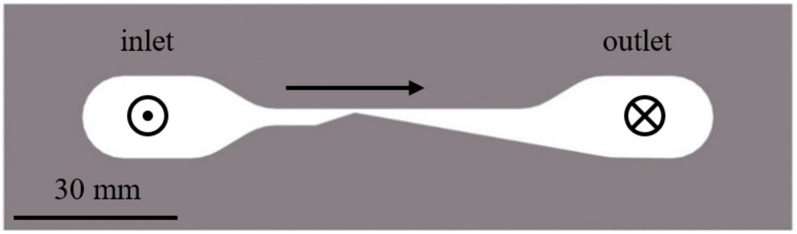
The experimental method is seen here only briefly, a more detailed study can be found in [8]. The set-up is illustrated in Figure 1. By sandwiching them between two acrylic glass plates, microchannels are constructed of 450 μm thick stainless-steel sheets that have a laser-cut convergent-divergent narrowing. The Venturi channel’s convergent angle measures 18° and the divergent angle is 10°, with a throat height of 675 μm. Both the channel entrance and exit are perpendicular to the cross-section plane, with the channel inlet on the left and the outlet on the right side of the channel.

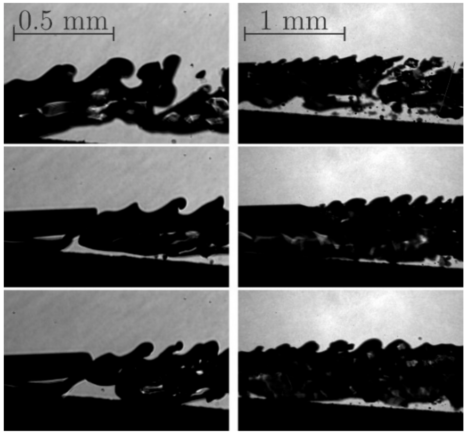
High-speed cameras (Photron SA-Z and Photron Mini AX200, Photron, Tokio, Japan) have captured cavitation images at a framerate of typically 200,000 fps in both the visible and X-ray light spectrum. Typical flow features that imply the formation of the Kelvin-Helmholtz instability in the channel are shown in Figure 2. The flow is from the left side to the right.

Figure 2 illustrates common microchannel representations of the Kelvin-Helmholtz instability. In particular, these images are from an experiment with a mass flow ($\stackrel{·}{\mathrm{m}}$) 9.15 g/s, a pressure difference between inlet and outlet (Δp) 4 bar, and a cavitation number (σ) of 1.24. A closer look at the flow conditions shows that the attached cavity first forms in the shape of a large single cavitation bubble extending downstream from the starting point until the pressure rises well above the saturation pressure—the presence of cavitation is like the supercavitation state. Kelvin-Helmholtz instability forms when the bubble approaches its maximum size. The ripple of the interface increases and the instability encircles the entire cavitation cloud while rolling up and induces its very rapid dissolution in the flow. The pattern then continues periodically.

The numerical simulation that provides further information in the creation of the Kelvin-Helmholtz instability and the cavitation dynamics in the microchannel is presented in the next section.

3. Numerical Procedure

A relatively straightforward simulation was carried out using the commercial Fluent 2020 R2 software package (Ansys Inc, Canonsburg, PA, USA). The solution was obtained with the Unsteady Reynolds-averaged Navier-Stokes (URANS) equations, with Reboud correction modified SST k-ω turbulence model and the Schnerr-Sauer cavitation model. The next section provides some more information.

3.1. Mesh

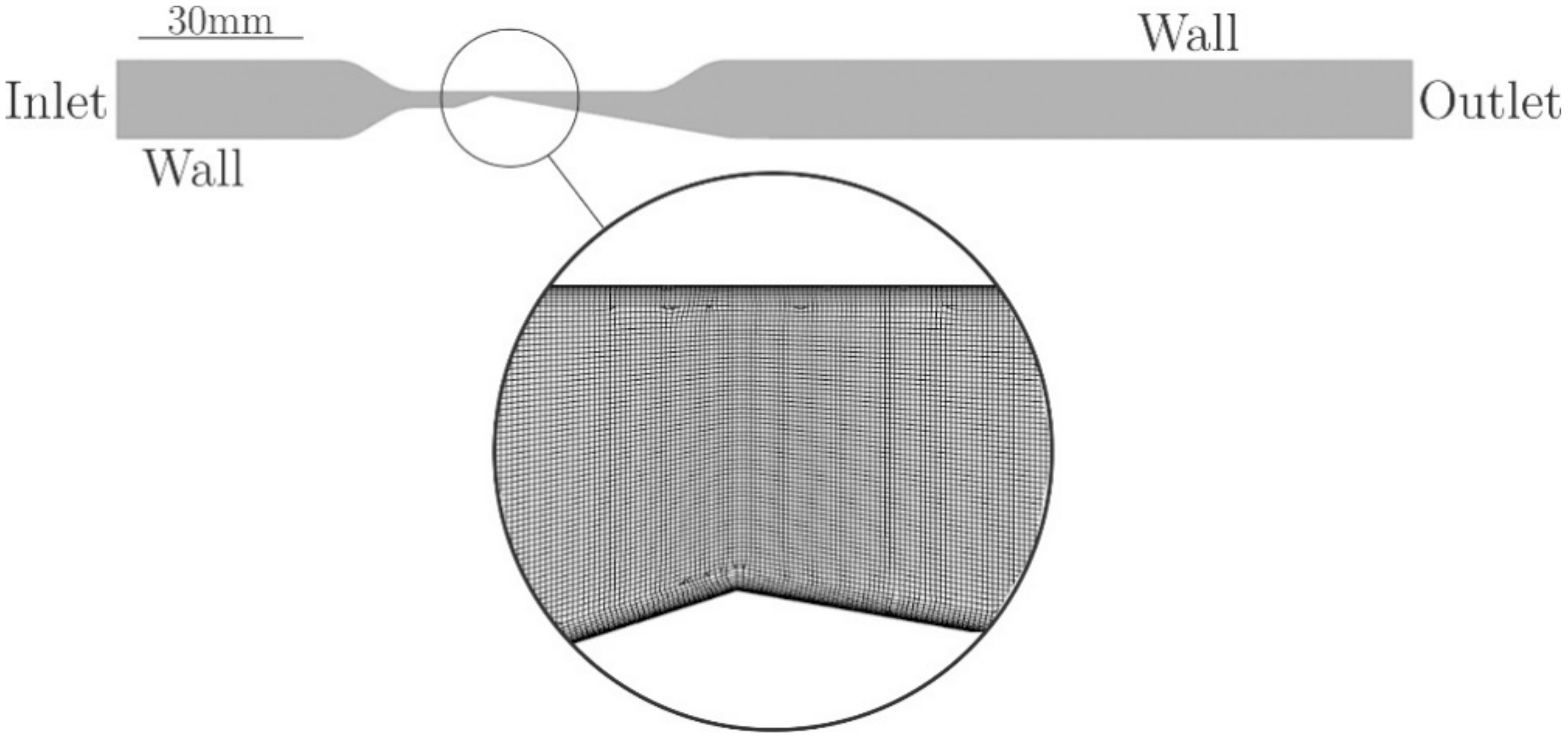
We regarded the matter two-dimensionally to promote the computation of the case and to expedite the simulation calculation. Thus, as seen in Figure 3, the channel inlet and outlet are modified appropriately. The structured computational mesh was used. The mesh independence was tested on 3 meshes while observing the average pressure difference Δp and the average cavity length l. The discretization error of less than 0.6% was calculated by Richardson extrapolation [9] for the medium mesh with around 160,000 cells at a flow rate of $\stackrel{·}{\mathrm{m}}$ = 9.03 g/s (

Table 1. Mesh independence study.

Mesh Size	Δp (bar)	l (mm)
~80,000	3.56	25.0
~160,000	3.71	25.6
~320,000	3.73	25.7

).

Along with the channel height, the final mesh had a constant number of 67 cells. Therefore, 10 μm is the height of an individual cell at the wedge apex. In relation to the geometry, the cells grow in the length to height ratio towards the inlet and the outlet of the domain. We have considered the boundary layer, where the overall thickness of the boundary layer of 50 μm was defined, with 10 layers and a growth rate of 1.2, which is a sufficiently small mesh to maintain the y+ values below 5.

3.2. Reynolds-Averaged Navier-Stokes (RANS) Equations

The Navier-Stokes equations are a set of partial differential equations, describing the conservation of momentum and mass for a viscous fluid flow motion. A direct numerical simulation, in which the Navier-Stokes equations are solved without a turbulence model, requires a huge amount of computing power because the whole range of spatial and temporal scales of the turbulence must be resolved. As this is not practical, averaging of variables is used. The idea behind averaging is the Reynolds decomposition, an instantaneous quantity decomposition into its time-averaged Φ and fluctuating quantities φ’(t) with zero mean value. Reynolds-averaged Navier-Stokes equations will be used in the form, that is generally accepted in the commercially available computational fluid dynamics (CFD) solvers. Here, the overline indicates a time-averaged variable, while the tilde indicates a density-weighted averaged or Favre-averaged variable [10]. The Favre-averaging method was selected because in the present case turbulent fluctuations lead to sizeable density fluctuations. The continuity equation is as follows, where ρ is the fluid density, t time, and U velocity vector, defined as $\mathit{U}={\left[U,V,W\right]}^{\mathrm{T}}$:

$$\frac{\partial \overline{\rho }}{\partial t}+\nabla ·\left(\overline{\rho }\tilde{U}\right)=0$$

(1)

The momentum equations in the x and y directions are as follows, where P is pressure, µ dynamic viscosity, u′, v′ and w′ velocity fluctuations of velocity vector U, while S_Mx and S_My represent momentum source terms in x and y directions, respectively

$$\begin{gathered} \frac{\partial \left(\overline{\rho }\overline{U}\right)}{\partial t}+\nabla ·\left(\overline{\rho }\overline{U}\overline{\mathit{U}}\right)=-\frac{\partial \overline{P}}{\partial x}+\nabla ·\left(\mu \nabla \overline{U}\right)+\left[-\frac{\partial \left(\overline{\overline{\rho }{u^{\prime }}^2}\right)}{\partial x}-\frac{\partial \left(\overline{\overline{\rho }{u}^{\prime }{v}^{\prime }}\right)}{\partial y}-\frac{\partial \left(\overline{\overline{\rho }{u}^{\prime }{w}^{\prime }}\right)}{\partial z}\right]+S_{Mx} \\ \frac{\partial \left(\overline{\rho }\overline{V}\right)}{\partial t}+\nabla ·\left(\overline{\rho }\overline{V}\overline{\mathit{U}}\right)=-\frac{\partial \overline{P}}{\partial y}+\nabla ·\left(\mu \nabla \overline{V}\right)+\left[-\frac{\partial \left(\overline{\overline{\rho }{u}^{\prime }{v}^{\prime }}\right)}{\partial x}-\frac{\partial \left(\overline{\overline{\rho }{v^{\prime }}^2}\right)}{\partial y}-\frac{\partial \left(\overline{\overline{\rho }{v}^{\prime }{w}^{\prime }}\right)}{\partial z}\right]+S_{Mx} \end{gathered}$$

(2)

For the accurate representation of cavitating flow details, some authors perform compressible flow simulations [11,12,13]. In the compressible case, the energy conservation equation is added to the above set of continuity and momentum equations. Also, equations of state of vapor and liquid are introduced. On the other hand, some authors have shown, that sufficient flow representation accuracy was obtained in the incompressible flow case, much decreasing the computational load requirements (for example [2,14]).

3.3. Turbulence Modeling

Increased available computational power has made possible advances in computational fluid dynamics, among them Large-Eddy Simulation (LES) and Detached-Eddy Simulation (DES). These relatively novel approaches are in research used to accurately resolve all scales of turbulent fluctuations, while for engineering purposes there is usually no need for such complexity. In above mentioned Reynolds-averaging models, turbulent fluctuations are not resolved, and the turbulence model is used instead. The k-ω and k-ε turbulence models are the most common models used to simulate mean flow characteristics for turbulent flow conditions. Both are two-equation models that provide a general description of turbulence utilizing two transport equations. The Menter’s Shear Stress Transport (SST) k-ω turbulent model [15], combines both k-ω and k-ε turbulence models such that it merges the robust, accurate, and less y+ sensitive performance of the k-ω model in the near-wall region with the solid freestream operation of the k-ε model in the far-field. Nowadays the SST k-ω turbulent model is the preferred two-equation turbulent model and the preferred model for a wide range of applications.

For the modeling of nonstationary cavitation flows, among them, periodic cavitation cloud shedding, two-equation turbulent models in the original form are not the preferred option. Two equation models prevent the reentrant jet from appearing at the rear of the cavitation cloud, all this being caused by too high prediction of turbulent viscosity. For a better non-stationary turbulence modeling performance, Reboud et al. [16] proposed a modification of the turbulent model. In the modification, the turbulent viscosity of the mixture is reduced in regions with high void fractions and the equation of turbulent viscosity becomes as follows, with k representing turbulence kinetic energy and ω specific turbulence dissipation rate:

$${\mu }_t=f\left(\rho \right)\frac{k}{\omega }$$

(3)

The density function is set by Equation (4), here indices l, v, m represent liquid, vapor, and mixture.

$$f\left(\rho \right)={\rho }_v+\frac{{\left({\rho }_m-{\rho }_v\right)}^n}{{\left({\rho }_l-{\rho }_v\right)}^{n-1}} n\gg 1$$

(4)

Various values were proposed for the exponent n. Coutier-Delgosha et al. [17] proposed value n = 10, while the described turbulent model extension was used and validated for various applications, among them in Venturi channel and a hydrofoil [2,3,18,19,20].

3.4. Two-Phase Flow Modeling

We more commonly use the concept of the homogeneous flow of the mixture for cavitation simulation, where the two-phase flow is assumed to be a single-phase flow of the liquid-vapor mixture. This helps one to solve only one motion equation since we consider the problem as a single-phase, but with the mixture’s properties. Accordingly, the properties of the liquid-vapor mixture are described by the proportion of the vapor phase, using the model suggested by Bankoff [21]. The mixture’s density is written:

$${\rho }_m=\alpha {\rho }_v+\left(1-\alpha \right){\rho }_l$$

(5)

where α denotes vapor volume fraction, and mixture’s dynamic viscosity is written as:

$${\mu }_m=\alpha {\mu }_v+\left(1-\alpha \right){\mu }_l$$

(6)

The equations of mass and momentum conservation are resolved in the model of the homogeneous flow of the mixture by the properties of the mixture, and the equation of phase fraction conservation must be solved:

$$\frac{\partial }{\partial t}\left({\rho }_v\alpha \right)+\nabla ·\left({\rho }_v\alpha u_v\right)=R_e-R_c$$

(7)

where R_e and R_c represent mass transfer source terms for evaporation and condensation, which account for the mass transfer between the phases of liquid and vapor in cavitation and are thus related to the growth and collapse of the vapor bubbles. According to the cavitation model used, their formulation varies.

3.5. Cavitation Model

We know multiple models of cavitation in which we can model liquid and vapor evaporation and condensation. Bubble dynamics models, introduced by Kubota et al. [22], where he used a linear portion of the Rayleigh-Plesset equation to explain the evolution of bubble radius as a function of surrounding pressure have been the most used cavitation models in CFD in recent years. The proportion of the vapor phase and hence the density of the mixture is calculated by bubble radius and bubble number density. Other cavitation models were derived relying on the pressure and bubble radius dependencies [23], based on the Rayleigh-Plesset equation. However, with all cavitation models, it is conditioned to specify parameters, such as the bubble number density or the initial size of the bubble, which are very hard to define. The Schnerr-Sauer [24] model is the cavitation model based on bubble dynamics that is most widely used in commercial CFD software packages, where the mass transfer source terms R_e and R_c (see Equation (7) are defined as:

when local pressure is equal to or smaller than vapor pressure—$p\le p_v$:

$$R_e=F_{evap}\frac{{\rho }_v{\rho }_l}{\rho }\alpha \left(1-\alpha \right)\frac{3}{R_b}\sqrt{\frac{2}{3}\frac{\left(p_v-p\right)}{{\rho }_l}}$$

(8)

when local pressure is larger than vapor pressure—$p>p_v$:

$$R_c=F_{cond}\frac{{\rho }_v{\rho }_l}{\rho }\alpha \left(1-\alpha \right)\frac{3}{R_b}\sqrt{\frac{2}{3}\frac{\left(p-p_v\right)}{{\rho }_l}}$$

(9)

where the default values of empirical calibration coefficients of evaporation F_evap and condensation F_cond are 1 and 0.2, respectively. To link the fraction of the vapor volume to the number of bubbles per liquid volume n_b, the Schnerr-Sauer cavitation model uses:

$$\alpha =\frac{n_b\frac{4}{3}\pi R_b^3}{1+n_b\frac{4}{3}\pi R_b^3}$$

(10)

The parameters that must be determined in this model are bubble radius R_b and bubble number density n. The compressibility of water and water vapor was not considered in the modeling.

3.6. Boundary Conditions

Modeling cavitating flow in the microchannel was performed at several mass flow rates. The boundary condition was set at the inlet of the Venturi channel computational domain as average velocity. The inlet turbulence intensity was set to zero. The vapor volume fraction at the inlet was set to zero also.

At the outlet of the Venturi channel computational domain the second boundary condition was set prescribing the absolute pressure 1 bar and backflow turbulence intensity 5% for all mass flow rates. The vapor volume fraction at the outlet was set to zero.

On all walls, the no-slip stationary wall boundary condition was used with a standard wall roughness model. The temperature was in all cases set to 20 °C.

3.7. Physics and Solver Settings

It is important to set proper simulation settings, as are the initial conditions from which to start the simulation, so we first performed simulations as single-phase simulations for each mass flow under stationary conditions. The outcomes were then considered as the initial conditions for further transient simulations. Numerical calculations were carried out using time-dependent Reynolds-averaged Navier-Stokes equations. Homogeneous water and water vapor mixture was considered and a Schnerr-Sauer cavitation model [24] with an evaporation pressure of 2340 Pa was used. A modified SST k-ω model, using the turbulent viscosity correction suggested by Reboud et al. [16] and Coutier-Delgosha et al. [17], mentioned above, was used for the turbulent model. For pressure and velocity coupling, the PISO algorithm [25] was used. We used the second-order upwind scheme [26] for spatial numerical discretization of solving hyperbolic partial differential equations for all but the pressure and volume fraction, providing more precise results with marginally higher computer resource usage compared to the first-order upwind scheme. The PRESTO interpolation scheme was used to discretize the pressure [27], and the first-order upwind scheme [26] was used for the discretization of the volume fraction. Time integration was modeled for transient solutions using the implicit transient formulation of bounded second-order.

The convergence criteria were established by evaluating the progression of various flow parameters (absolute pressure at the inlet and outlet, and velocities at the microchannel inlet, outlet, and throat). Following the sum of the imbalance of transport equations between iterations for all cells in the computational domain, the observed flow parameters were converged when falling below 10⁻⁵ of the iterative numerical solution of the individual equations at each time step of the simulation. The iteration error was estimated to be less than 0.02%. By assessing its effect against the average pressure difference and the cavity length, the size of the time step was obtained. There was little difference in these parameters if the time step was shorter than 5 μs, but a shorter one—1 μs was ultimately chosen for observation of the Kelvin-Helmholtz instability. We conducted 50 ms of computational modeling for each case, where the last 30 ms was applicable for further analysis.

4. Results

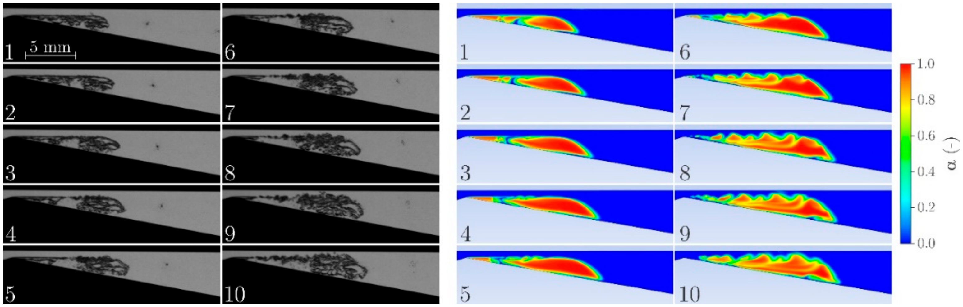
First, we assess the capability of the numerical simulation to capture the general cavitation dynamics which was observed inside the microchannel—more specifically the onset of the Kelvin-Helmholtz instability (Figure 4). The flow is from the left to the right, the time difference between the images is 100 μs.

The experiment and simulation both reveal the same story, but in the case of simulation, the Kelvin-Helmholtz instability is more pronounced and can be understood better and described more in detail.

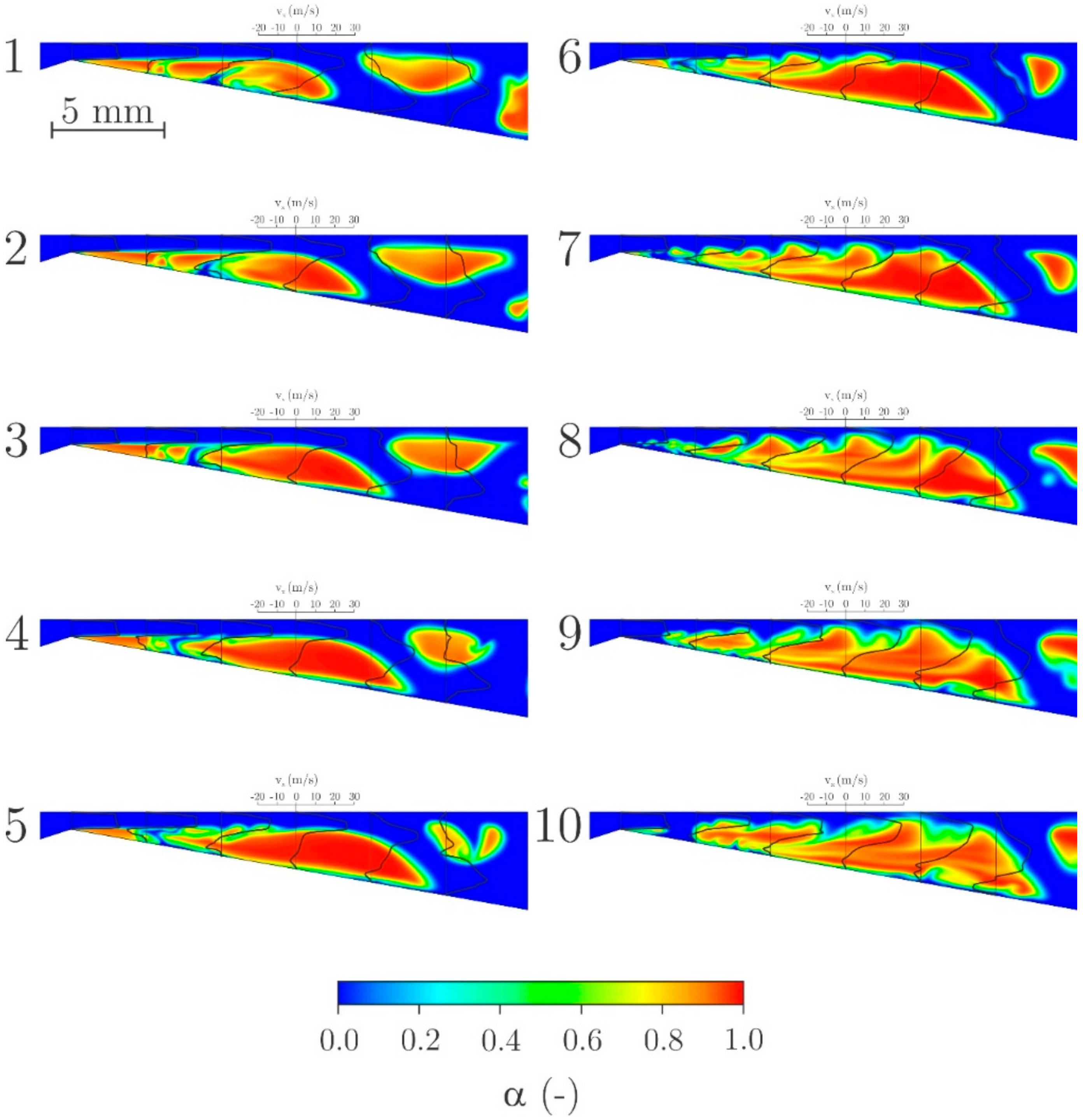
In Figure 5, the development of the Kelvin-Helmholtz instability is shown with velocity profiles drawn over at cross-sections at horizontal intervals of 3 mm in the downstream direction, starting at the wedge apex.

Fluid flow velocity at the throat of the Venturi microchannel is 30 m/s, where liquid flows over the cavity and descents afterward towards the bottom wall of the channel, where the flow divides into the upstream and downstream flow (1). Vapor fraction α profiles for both phases are approximately uniform in both the fluid and vapor layers. They are however discontinuous at the straight interface between the two (step 1). Shear stress acts on the fluids due to discontinuity of the velocity gradient (velocity gradients are shown by the black line in Figure 5), while vapor gradient locally promotes the generation of instabilities and vorticity. The backflow due to the presence of the adverse pressure gradient at 6 mm downstream from the throat in the vapor phase increases from a peak value of 5 m/s to 13 m/s (step 2), which further increases shear stress. Increased shear stress between the liquid and cavity interface results in the formation of ripples on the interface, while the reentrant jet progresses further upstream. The attached cavity expands and reaches its full size (step 2) and shortly thereafter (100 µs) in step (3) one can see the first beginnings of ripples on the upper edge area of the vapor phase (approx. 6 mm from the Venturi throat). This promoting the formation of instabilities (step 3) in addition to the already present vertical shear stress between the liquid flow and the cavity interface enables the formation of Kelvin Helmholtz instability.

In step (4), 300 µs after the start of the instability formation process, we already observe the formation of unstable local turbulent structures approx. 6 mm from the Venturi throat, which are now confined to the shear layer. Due to their limited size, velocity gradients in step (4) are still unchanged in comparison to step (1) and the rolling motion of turbulent structures is not yet recognized. With time, the surface becomes more and more deformed from the original straight boundary interface, and turbulent structures grow in size and number (step 5). It seems that the vapor region is affected by the formation of turbulent structures, here velocity, density, and momentum are low. Velocity profiles in the vapor region change with instabilities continuously protruding deeper in the vapor region, finally leading to the situation in step (5).

Instabilities in the vapor phase continue to grow from step (5), and the region of high pressure between the cavities moves in the opposite direction to the main flow towards the Venturi throat, from approx. 4 mm in step (5) to approx. 2 mm in step (6). Advance in the direction opposite is related to the presence of the adverse pressure gradient (step 6), with instabilities and turbulent eddies in later steps reaching the Venturi throat section and causing full cavity separation and partial destruction of the vapor region in the vicinity of the throat. The vapor phase in the vicinity of the throat does not reappear until step (10) 900 µs after the start of the process. In steps (7–9) we notice the change of the velocity profiles, caused by the separation of the cavity from the Venturi throat and hence smoothing of the velocity profiles in the horizontal direction. The region of constant velocity near the upper Venturi section wall is reduced and the velocity profiles in horizontal direction become skewed. Regions of backflow are reduced in size and intensity. In steps (7–9) generation of Kelvin Helmholtz instabilities increase further downstream of the detached cavitation cavity. Finally, the entire detached cavitation cloud becomes engulfed in the border instabilities. In addition to the change of velocity gradient, the vapor fraction α in the vertical direction becomes non-homogeneous and areas of slightly higher vapor fraction α can be traced to the region where instabilities were initially formed. The detached cavitation cloud together with all instabilities continues to flow downstream and finally dissipates (not shown in this sequence).

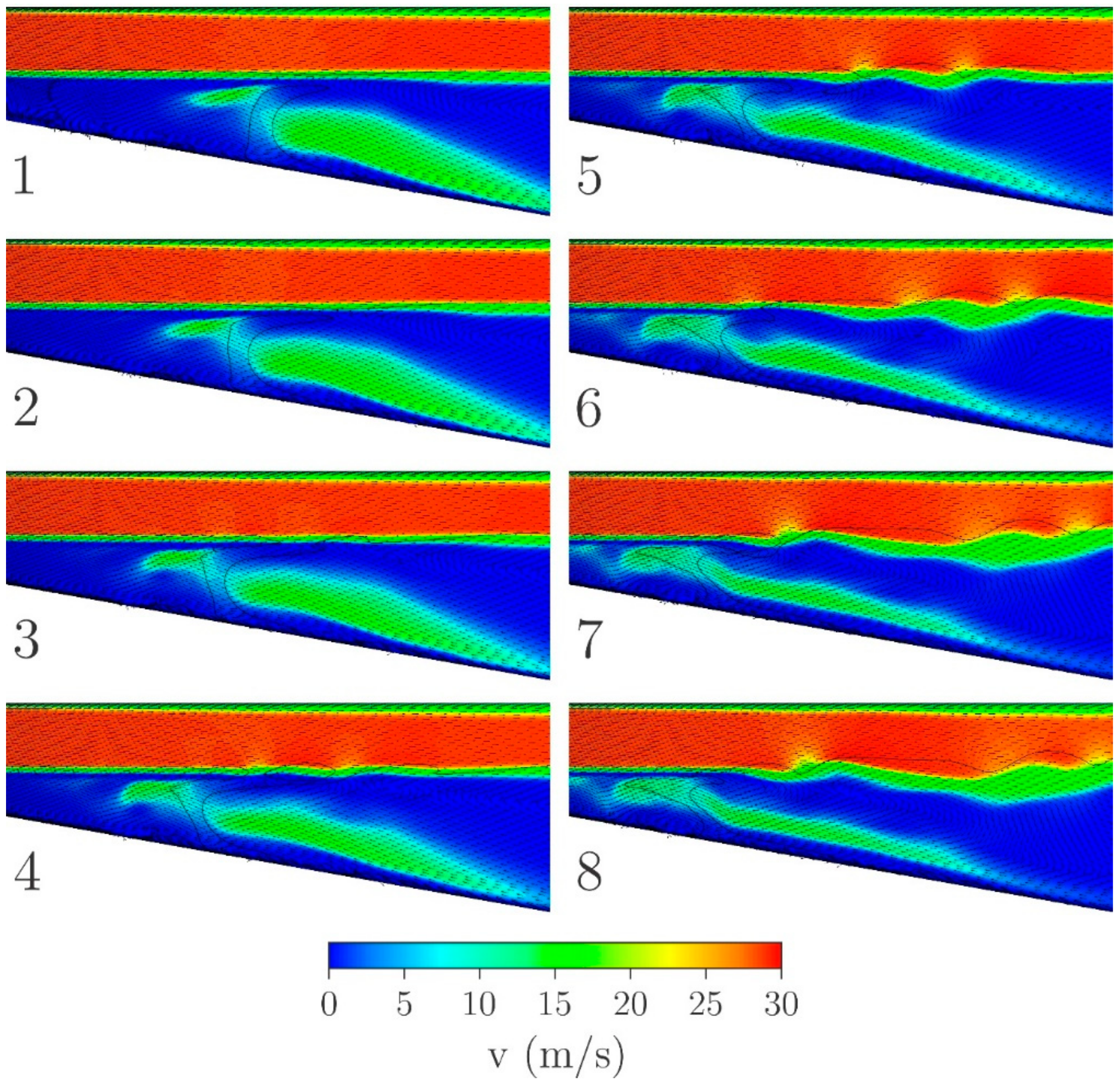
In step (10), 900 µs after the start of the instabilities formation, cavitation cavity is again formed at the Venturi throat section and the entire process is about to continue in a quasi-periodic way. More insight into the instability formation process may be gained from Figure 6, which shows an enlarged segment of the Venturi section relative to Figure 5.

Velocity vectors reveal the presence of the turbulent eddies within the vapor phase and their interaction with the main flow above the discontinuity of the horizontal velocity. Figure 6 also shows contours of 10% vapor region location.

Step (1) shows the initial situation with a turbulent eddy on the right side of the observation region. Just next to the lower limit of 10% vapor region is the turbulent eddy impingement point on the shear layer. On the left of the 10% vapor fraction region, we observe the backflow, while on the right the turbulent eddy rotation causes the flow velocity to be in the direction of the main flow. Impingement point marks the position of the large variation of the shear stress gradient, on the left of the impingement point, the stress is higher than on the right. The horizontal 10% vapor fraction region limit of the velocity discontinuity is just above the impingement point. The transition from step (1) to step (2) is marked with an additional depression of the horizontal 10% vapor fraction region limit. The location of the impingement point and the horizontal 10% vapor fraction region has moved to the right in step (2) relative to step (1), while the lower 10% vapor fraction region has widened from the original location in step (1) to the newly established impingement point of step (2).

As the instability process continues in step (3) we observe gradual folding of the lower 10% vapor fraction limit, even before we notice significant variations in the velocity within the shear layer. We, therefore, speculate that the vapor fraction properties influence the instability process through the variation of the flow density and the transfer of the momentum. In step (3) we notice velocity variations within the main flow, corresponding well to the vapor fraction variations in intensity and location. The process, first observed in step (3) continues with step (4) showing increased spatial variations of the vapor fraction, followed by velocity variations in the main flow. As a consequence, turbulent eddy, first responsible for impinging the shear layer, is decayed into two turbulent eddies with an additional one formed near the location of the original impingement point. The location of the lower 10% vapor fraction region limit has moved in the direction of the Venturi section throat.

Steps (5) to (8) show markedly increasing folding of the shear layer, coupled with the additional breaking of the turbulent eddy into several smaller ones, including interactions among neighboring turbulent eddies. Gradually location of the lower 10% vapor fraction region moves further left towards the throat finally causing the detachment of the cavitation cloud as described above for Figure 5. Folding of the shear layer is coupled with its gradual thickening. Location, where the gradient of shear layer folding is high, is accompanied by the regions of main flow deceleration and hence variations of the velocity and pressure in the main flow.

5. Conclusions

Numerical simulation has provided additional insights into the formation of Kelvin-Helmholtz flow instabilities in the Venturi section. The process is being able to cause the shedding of cavitation clouds similar to the re-entrant jet or shockwave cases. Results conform well to the available experimental data.

The formation of Kelvin-Helmholtz instabilities is determined by the large vertical variations in the shear stress, vapor fraction, and the different physical properties of liquid and vapor regions. The vapor with its much lower density and momentum is more impacted by the instabilities creation as the liquid region. This promotes perturbations and the development of the turbulent eddies in the vapor region. Turbulent eddy impingement point on the shear layer point marks the position of the large variation of the shear stress gradient. We observed the folding of the lines of constant vapor fraction within the shear layer even before any velocity changes were noticed. Thus, the vapor fraction properties may influence the Kelvin-Helmholtz instability formation process through the variation of the density and the transfer of the momentum. As instabilities grow further, adverse pressure gradient and velocity lead to the detachment of the cavitation cloud together with all instabilities.

In both layers, Kelvin-Helmholtz instabilities for the case of cavitation in the Venturi section express less pronounced rolling motion and are less periodic and symmetric in comparison with their more well-known occurrences. This perhaps was the reason that Kelvin-Helmholtz instability was not recognized before as a possible source of the cavitating flow instabilities and cavitation cloud shedding.

More experimental and numerical studies will be required in the future to better understand the formation of Kelvin-Helmholtz flow instabilities in cavitation flow and their role in the cavitation shedding process.